Implementing Higher Order Dynamics into the Ice Sheet Model SICOPOLIS

(1)

UPTEC F11 015

Examensarbete 30 hp

Februari 2011

Implementing Higher Order

Dynamics into the Ice Sheet

Model SICOPOLIS

(2)

Teknisk- naturvetenskaplig fakultet UTH-enheten Besöksadress: Ångströmlaboratoriet Lägerhyddsvägen 1 Hus 4, Plan 0 Postadress: Box 536 751 21 Uppsala Telefon: 018 – 471 30 03 Telefax: 018 – 471 30 00 Hemsida: http://www.teknat.uu.se/student

Abstract

Implementing Higher Order Dynamics into the Ice

Sheet Model SICOPOLIS

Josefin Ahlkrona

Ice sheet modeling is an important tool both for reconstructing past ice sheets and predicting their future evolution, but is complex and computationally costly. It involves modeling a system including the ice sheet, ice shelves and ice streams, which all have different dynamical behavior. The governing equations are non-linear, and to capture a full glacial cycle more than 100,000 years need to be simulated. To reduce the problem size, approximations of the equations are introduced. The most common

approximation, the Shallow Ice Approximation (SIA), works well in the ice bulk but fails in e.g. the modeling of ice streams and the ice sheet/ice shelf

coupling. In recent years more accurate models, so-called higher order models, have been constructed to address these problems. However, these models are generally constructed in an ad hoc fashion, lacking rigor. In this thesis, so-called Second Order Shallow Ice Approximation (SOSIA) equations for pressure, vertical shear stress and velocity are implemented into the ice sheet model SICOPOLIS. The SOSIA is a rigorous model derived by Baral in 1999 [3]. The numerical solution for a simple model problem is compared to an analytical solution, and benchmark experiments, comparing the model to other higher order models, are carried out. The numerical and analytical solution agree well, but the results regarding vertical shear stress and velocity differ from other models. It is concluded that there are problems with the model implemented, most likely in the treatment of the relation between stress and strain rate.

Examinator: Tomas Nyberg Ämnesgranskare: Per Lötstedt Handledare: Nina Kirchner

(3)

1 Introduction

1.1 Ice Sheets

The cryosphere (glaciers, ice caps, ice sheets, ice shelves, sea ice, frozen ground etc.) plays an important role in the global climate system. Concern about the evolution of large ice masses in response to global warming has risen, especially since the latest IPCC report was published in 2007 [31]. Ice masses have a strong impact on the surface energy balance of the Earth through feedback mechanisms such as e.g. the ice-albedo feedback, according to which white areas reflect more light/energy back into space while dark ones absorb energy. Once glaciated, ice covered areas are thus likely to locally generate an even colder climate through the feedback mechanism, and vice versa [31]. The mass balance of ice masses is also intimately connected to sea-level rise. The two largest ice masses on earth are the Antarctic Ice Sheet and the Greenland Ice Sheet. If the entire Antarctic Ice Sheet were to melt, the melt water would cause the sea level to rise by about 57 m. If the Greenland Ice Sheet would melt, the contribution to sea level rise would be about 7 m [30, 2, 29, 32].

An ice sheet is an ice mass that covers an area of 50, 000 km2 _{or more [13],}

if less it is referred to as an ice cap, e.g. Vatnaj¨okull in Iceland. The only ice sheets present today are the Greenland Ice Sheet (1, 710, 000 km2_{) and the}

Antarctic Ice Sheet (14, 000, 000 km2) [31]. When ice from an ice sheet or ice cap flows into the ocean and becomes afloat it is called an ice shelf. The world’s largest ice shelf is the Ross Ice Shelf in Antarctica. It has an area of almost 500, 000 km2_{, i.e. about the size of France [23]. The boundary between the ice}

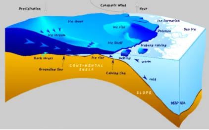
shelf and the grounded ice is called the grounding line. Because of the size, ice sheets are of great interest in the context of climate change, but ice shelves are also important to understand since they affect the dynamics of the connected ice sheet. We shall in the following focus on ice sheets only. In an ice sheet there can be narrow bands of fast flowing ice, referred to as ice streams. These are responsible for massive discharge of ice from the interior ice sheet to its coastal margin, and interlink terrestrial and marine ice masses. Figure 1 shows a sketch of an ice sheet, including an ice stream, flowing out into an ice shelf. The velocity in an ice stream can be well over 10, 000 m a year while the slow moving bulk of the ice generally moves some tens of meters a year [20]. Figure

2 shows how the structure of the ice surface in an ice stream differs from the

surface of the slow moving ice because of the high velocity. There is a sharp transition between the two different flow regimes that apparently takes place in a thin boundary layer.

An ice mass can be polythermal, i.e. comprised by both cold and temperate ice. Cold ice is ice with temperatures below the pressure melting point and temperate ice has a temperature at the pressure melting point and is a mixture of ice and water.

1.2 Ice Sheet Modeling

The response of ice sheets to climate change is complex and numerical model-ing is an important tool in understandmodel-ing the dynamics of ice sheets, both in reconstructions of former ice sheets and in predicting their future behavior in response to climate warming. There are several existing large-scale models that

(5)

Figure 1: An ice sheet flowing outwards to the ocean and forming an ice shelf. In the ice sheet there is an ice stream, where the ice flows faster. Picture by Grobe [40].

Figure 2: Satellite image of a part of Ice Stream B, Antarctica. Flow direction in the picture is from the upper right to the lower left corner. The surface of the ice stream is highly irregular, and a sharp boundary separates the bulk inland ice (slowly moving) from the fast moving ice stream. From British Antarctic Survey [38].

(6)

are generally successful in simulating ice sheets, but as all models they have shortcomings. In particular, there are weaknesses in the modeling of basal flow processes, the coupling of ice marginal dynamics and inland ice dynamics, ice sheet-ocean interaction, and ice streams. These processes are important to un-derstand since they are related to the ice sheet sensitivity and response time. Ice sheets are thus more vulnerable to climate change than current models suggest and predictions of future sea-level rise may very well be underestimated [31]. This work is part of a project focusing on improving the modeling of ice stream dynamics, embedded in the overall ice sheet dynamics. Figure 3 illustrates the poor modeling of ice streams by comparing real surface velocities with those computed by the ice sheet model SICOPOLIS (SImulation COde for POLy-thermal Ice Sheets). Other ice sheet codes suffer from similar shortcomings when trying to simulate ice stream behavior in a forward manner (e.g. Elmer [34] [37]). Inverse modeling strategies have thus recently become very popular, with inversion for the ice stiffness parameters of ice shelves and ice stream basal parameters being most common [24, 21, 10].

(a) Satellite image (b) Model output.

Figure 3: Surface velocities at the Greenland Ice Sheet. (a) is a satellite image showing ice velocities (surface) at the Greenland Ice Sheet during winter 2010 (Image by Joughin et al. [20]). Blue/purple colors show high velocities. (b) shows model output from a simulation run with SICOPOLIS, using a horizontal grid resolution of 20 km. Hot colors are high velocities. The satellite image shows ice streams that are not showing in the output from the ice sheet model SICOPOLIS. In particular, the North Eastern Greenland Ice Stream (marked by a red arrow) is clearly visible in the satellite image, but does not show in the model output. For esthetic reasons figure (b) only shows velocities up to 3000 m/a, but the maximum velocity is almost 7000 m/a.

Indeed, ice sheet modeling is complicated, because the individual compo-nents (grounded inland ice sheet, fast flowing ice streams, attached floating ice shelves) all exhibit different dynamical behavior under external forcing. While the individual subsystem can be modeled in isolation, modeling of the coupled

(7)

system is challenging since it requires careful matching of the different dynam-ical regimes in the transition zones, which themselves are dynamdynam-ically evolving in space and time. This is an issue particularly since large scale ice sheet mod-els typically are based on the so-called Shallow Ice Approximation (SIA) [17] to simplify the governing equations. The SIA balances basal drag at the ice base with vertical shear stress, disregarding other stress terms such as horizon-tal plane (HP) shear stress and normal stresses, since these are small in the main part of an ice sheet. However, in ice shelves and in many ice streams, the basal drag and hence the vertical shear stress is reduced, increasing the relative importance of normal and HP shear stress. In an ice shelf the low basal drag is due to the fact that the ice floats in the ocean, and that there is almost no friction at the ice/ocean interface. For ice streams, the reduction in basal drag is poorly understood and can be explained by several different processes, such as basal melt water or deforming till [1, 33]. Figure 4 shows how the influence of basal drag and vertical shear stress is different in ice sheets, ice shelves and ice streams. Since HP shear stress and normal stresses are not considered in the SIA, the modeling of ice streams and the ice sheet/ice shelf coupling fails.

The SIA is used because it is relatively simple and reduces computation time, but in order to treat ice streams and the grounding line area correctly, so-called higher order dynamics is required [8]. The use of higher order dynamics would also allow for a finer grid resolution than what is possible when using the SIA-equations. An often used horizontal grid resolution is 20 km [4]. The smallest objects that can be resolved by this grid is then 40 km, corresponding to the Nyquist wavelength λN. However, in order for the SIA to be accurate, the data

needs to be smoothed even more, so that the variations are much coarser than the Nyquist wavelength.

1.3 Aim of this Work

This work aims to implement higher order dynamics, or to be specific: the so-called second order shallow ice approximation (SOSIA) equations for pres-sure, vertical shear stress and velocities, into the ice sheet model SICOPO-LIS. SICOPOLIS is a large-scale, three-dimensional, thermodynamically cou-pled model based on the SIA [12] and is the only code applicable to polythermal ice. SICOPOLIS is described further in section 4.1. Until recently, no rigorous ’second order ice sheet models’ existed, but there is now one under development by Egholm [9]. His implementation is however quite different from the one in this work.

The second order equations that are to be implemented in this project have been derived by Baral in his doctoral thesis in 1999 [3]. These equations are not in a form suited for direct implementation and further derivations are thus required in this work. The present work will be continued as a doctoral thesis and groundwork that will make future work easier is carried out here. The new model will be validated by comparing to an analytical solution and by carrying out the benchmarks experiments from the ’Ice Sheet Model Intercomparison Project for Higher-Order ice sheet Models’ (ISMIP-HOM), convened by Pattyn and Payne [42, 26]. The updated model will then be applied to the Greenland Ice Sheet and compared to results obtained by the SIA-model.

To limit this project, temperate ice is not considered and the temperature is held constant, thus the equations governing the temperature are not upgraded

(8)

(a) An ice sheet becoming afloat to form an ice shelf at the marine margin.

(b) An ice stream within an ice sheet, flowing out into an ice shelf.

Figure 4: (a) shows an ice sheet becoming afloat to form an ice shelf at the marine margin. The slow moving ice in an ice sheet often adheres to the bedrock, causing the velocities at the base to be lower than at the ice surface. This causes large vertical shear stress, since velocities and stresses are related through Glen’s flow law, see section 2. In the ice shelf, the ice rests on the ocean and the vertical shear is not dominant. (b) shows an ice stream within an ice sheet. In ice streams, basal conditions often lower the basal drag such that horizontal plane shear and normal deviatoric stresses become comparable to the vertical shear stress.

(9)

from the SIA to the SOSIA. Since the temperature influences the material prop-erties of the ice (especially the viscosity), this simplification will limit the accu-racy of the modeled ice dynamics. Furthermore, a no slip boundary condition is applied at the ice base and the lithosphere is assumed to be in isostatic equi-librium. Only ice sheets (not ice shelves) are considered.

2 Ice Sheet Modeling in a Continuum

Mechan-ical Framework

2.1 Introduction

In the following subsections, the theory presented in the book Advances in

Geo-physical and Environmental Mechanics and Mathematics by Greve and Blatter,

2009 [13], is described.

The ice sheet is bounded by the atmosphere at the free surface, h, and by the bedrock at the ice base b. It can also be coupled to an ice shelf, but as already mentioned, ice shelves are not considered in this work. To some extent, the lithosphere resting on the asthenosphere is modeled as well in order to properly account for heat conductivity and the deformation of the ice base/rock interface under the load of ice [13]. The consideration of layers of temperate ice adds an internal boundary, the so-called cold-temperate transition surface (CTS), zmto

the ’usual’ external boundaries, namely the free surface, h and the ice base, b. All of these boundary surfaces evolve in time and space. Figure 5 shows the different domains and boundaries in the model.

Figure 5: Domains and boundaries in the model. h is the ice surface, zmthe position

of the CTS, b the ice base and br the underside of the lithosphere.

The equations in the temperate ice region are more complicated than in the cold ice since there are two phases present: ice and water. These equations and the extra boundary condition at the CTS will not be presented here since temperate ice is not considered in this work. For completeness of the theory

(10)

regarding cold ice, the equation governing the energy is however also described even though only isothermal conditions are considered during implementation.

2.2 Ice Dynamics: Governing Equations and Boundary

Conditions

The set of equations governing the behavior of large natural ice masses consists of the balance equations and the constitutive equations. Together, they are called the ’field equations’ [17, 13]. Balance equations describe general laws of conservation that must be fulfilled for any material body (e.g. conservation of mass, linear and angular momentum and internal energy), while constitutive equations introduce material specific behavior to the balance equations. These equations together with the boundary conditions determine the problem. 2.2.1 Balance Equations

Under the assumption that we have a homogeneous, single-constituent material for which angular momentum is assumed to be obtained from taking the cross-product of linear momentum and some distance vector (i.e., we assume a so-called non-polar continuum) the general balance equations comprise the balance of mass, linear momentum and internal energy and read

0 = ˙ρ + ρdiv v, (1)

ρ ˙v = div T + ρg, (2)

ρ ˙ε = −div q + T · D + ρr. (3)

The quantities arising in the above equations are the mass density, ρ, the velocity field, v, the Cauchy stress tensor, T , the acceleration due to gravity, g, the internal energy density, ε, the heat flux vector, q, the energy supply density, r, and the strain rate tensor, D. D is by definition symmetric, D := sym∇ v.

The superposed dot in the equations denotes the material time derivative given by

•˙ = _∂t∂ (•) + (∇ •) · v (4)

where t denotes time. Note that there is no balance of angular momentum – for non-polar continua, the balance of angular momentum reduces to a symmetry condition on the stress tensor T in the balance of linear momentum. The symmetry of the Cauchy stress tensor is tacitly a priori assumed in almost all glaciological applications [25].

2.2.2 Constitutive Equations

Material specific behavior is introduced by prescribing so-called constitutive functions for the following quantities: the Cauchy stress T , the internal energy

ε and the heat flux q. Assuming that we deal with cold ice only, one typically

regards ice as being incompressible (density preserving), implying ρ = const. [17, 25, 13] or

(11)

With this, the Cauchy stress tensor T is rewritten as

T =_{−pI + T}E (6)

where p is the scalar pressure field and TE is the so-called extra-stress tensor which satisfies tr TE = 0, that is, the sum of the diagonal elements of TE vanishes due to the incompressibility assumption. Moreover, it is commonly assumed ab initio that acceleration terms in the balance of linear momentum can be neglected, ρ ˙v ≈ 0 (e.g. Paterson [25]). Here, this term is however

kept until section 2.3.1. Another common assumption is that energy supply is neglected, leading to r ≈ 0. According to Paterson [25], only one percent of

the incoming radiation reaches a depth of 1 m in the snow pack. With these assumptions, we only have to specify constitutive relations for the extra stress

TE, the heat flux q and the internal energy ε. This is commonly done as follows: the extra stress is linked to strain rate via Glen’s flow law, heat flux is modeled according to Fourier’s law, and changes in internal energy are related to changes in temperature T . Note that T! _{= T}_{− T}

M is the pressure melting point (TM)

corrected temperature.

D = E_A(T!)f (σ)TE, (7)

q = _{−κ(T )∇ T,} (8)

˙ε = cp(T ) ˙T . (9)

In equation (7) the factor EA(T!_{)f (σ) is related to viscosity as}

1

η = 2EA(T

!_{)f (σ),} ₍₁₀₎

where η is the viscosity. E ≥ 0 is the enhancement factor which can be set

to values greater than 1 to account, for instance, for the increased softness of glacial dust-containing ice compared with ordinary interglacial ice. A(T!_{) is}

the so-called rate factor, which through its dependence on the pressure melting point corrected temperature T! _{accounts for how the viscosity depends on}

tem-perature. The rate factor_{A can vary by several orders of magnitude. f(σ) is} the so-called creep response function and its argument σ, the effective stress, is the square root of the second invariant of the extra stress tensor, defined by

σ2= 1 2tr (T E₎2₌ ₍₁₁₎ = (tExz)2+ (tyzE)2+ (tExy)2+ 1 2 ! (tExx)2+ (tEyy)2+ (tEzz)2 " ,

where tij denotes components of the stress tensor T . See figure 5 for the

di-rections of x, (y) and z. Choosing f (σ) = (σ)n−1 _{with n = 3 is referred to as}

Glen’s flow law. A problem in using Glen’s flow law is that the creep function

f is zero for zero effective stress σ, leading to an infinitely large viscosity. To

avoid this, a modified flow law with an additional finite-viscosity parameter is required, which is further discussed in sections 2.3.3 and 5.3. In equation 8 and 9, κ is the coefficient of heat conductivity and cp is the specific heat.

(12)

Inserting the constitutive equations and Glen’s flow law into the balance equations yields the following field equations:

0 = div v, (12) ρ ˙v = _{−∇ p + div T}E+ ρg, (13) ρcp(T ) ˙T = ρcp(T ) # ∂T ∂t + (∇ T )v $ = div (κ∇ T ) + tr (TE· D) = (14) = div (κ∇ T ) + 2EA(T!_{)f (σ)σ}2_.

2.2.3 Boundary Conditions at the Free Surface

Following Greve and Blatter [13], the following boundary conditions are pre-scribed for the stress and the temperature at the free surface:

Tice· n = Tatm· n = −patmn + τwind≈ 0, (15)

Tice= Tatmosphere, (16)

where patm is the atmospheric pressure and τwind denotes stresses related to

the wind. Both these terms are neglected in SICOPOLIS. The evolution of the free surface is given by

∂h ∂t + vx ∂h ∂x+ vy ∂h ∂y − vz= Nsa ⊥ s, (17)

where vi denotes velocity components, Nsthe norm of the gradient of the free

surface and a⊥

s the accumulation-ablation function, i.e. the ice volume flux

through the free surface. Accumulation and ablation are related to precipitation and temperature.

2.2.4 Boundary Conditions at the Base At the ice base the stress is

Tice· n = Tlith· n − ρa⊥b (vlith− vice)≈ Tlith· n. (18)

Here the advective term is negligible. Since the stress in the lithosphere is not known, this condition is not useful. Instead the velocity at the base is prescribed. If the ice is frozen to the base, a no slip condition is used. If the ice is temperate at the base, a sliding law is needed. In this work, a no slip condition is used for simplicity. There is not enough data available regarding the basal temperature, and so the temperature can not be described directly in cold ice. If the kinetic energy is neglected, the boundary conditions is given by Fourier’s law of heat conductivity instead:

(13)

Here q⊥

geo is the component of geothermal heat flux perpendicular to the base

and κ is the heat conductivity. For temperate ice, it is given that the ice is at the pressure melting point Tm:

Tice= Tm, (20)

The condition for the evolution of the base follows as

∂b ∂t + vx ∂b ∂x + vy ∂b ∂y − vz= Nba ⊥ b , (21)

where Nbis the norm of the gradient of the base and a⊥b is the basal melting rate,

or the ice volume flux through the base (meltwater penetrates the underlying ground).

2.3 What is the Shallow Ice Approximation and Higher

Order Dynamics?

The above described equations are the so-called full Stokes equations. It is too computationally costly to solve these equations for an entire ice sheet and possibly hundreds of thousands of years; thus the SIA is widely used instead [19, 36, 35]. The SIA is based on the assumption that an ice sheet is shallow (i.e. the areal extent is much greater than the thickness). As mentioned in the introduction, the SIA does not properly model ice sheet dynamics such as ice streams and the ice sheet/ice shelf coupling. This motivates the implemen-tation of higher order dynamics, as the SOSIA-equations. The SIA, as well as the SOSIA, is derived from scaling of the full Stokes equations followed by perturbation expansion. This procedure is described in the sections below. 2.3.1 Scaling

The procedure below follows the one described in Greve and Blatter [13]. In scaling the full Stokes equations, the variables are non-dimensionalized and as a scaling parameter the aspect ratio, (, is used. The aspect ratio is the typical vertical extent of the ice sheet [H] divided by the typical horizontal extent [L] and is for an ice sheet usually of the order of 10−3. Brackets denotes typical values. For brevity of presentation, only results for the momentum balance will now be considered. In component form, the balance of linear momentum (equation (13)) is ρ ˙vx = − ∂p ∂x + ∂tE xx ∂x + ∂tE xy ∂y + ∂tE xz ∂z , ρ ˙vy = − ∂p ∂y + ∂tE xy ∂x + ∂tE yy ∂y + ∂tE yz ∂z , (22) ρ ˙vz = − ∂p ∂z + ∂tE xz ∂x + ∂tE yz ∂y + ∂tE zz ∂z − ρg.

(14)

To scale these equations the following transformations are used: (x, y) = [L](˜x, ˜y), z = [H]˜z, (vx, vy) = [VL]( ˜vx, ˜vy), vz = [VH] ˜vz, t = ([L]/[VL])˜t, (23) p = ρg[H]˜p, (tExz, tEyz, σ) = (ρg[H](˜tExz, ˜tEyz, ˜σ), (tExx, tEyy) = (2ρg[H](˜tExx, ˜tEyy), (tExy, tEzz) = (2ρg[H](˜tExy, ˜tEzz), ( = [H]/[L] = [VH]/[VL], F = [VL]2/g[L].

Tilde denotes dimensionless quantities. The complete presentation of how all variables are non-dimensionalized is given in for instance Baral et al., 2001 [4]. For the typical vertical and horizontal velocities it holds that

[VH]

[VL]

= (. (24)

Inserting the expressions in (23) into (22) yields

F (ρ ˙˜vx = − ∂ ˜p ∂ ˜x+ ( 2∂˜tExx ∂ ˜x + ( 2∂˜t E xy ∂ ˜y + ∂˜tE xz ∂ ˜z , F (ρ ˙˜vy = − ∂ ˜p ∂ ˜y + ( 2∂˜t E yy ∂ ˜y + ( 2∂˜t E xy ∂ ˜x + ∂˜tE yz ∂ ˜z , (25) F (ρ ˙˜vz = − ∂ ˜p ∂ ˜z+ ( 2∂˜tExz ∂ ˜x + ( 2∂˜t E yz ∂ ˜y + ( 2∂˜tEzz ∂ ˜z − 1,

where terms multiplied by powers of ( are considered to be small. The scaled equations illustrate the assumption that the normal deviatoric stress in the x-direction and the HP shear stress are of less importance than the vertical shear stress. This is generally true for an ice sheet, except for where there are ice streams. The Froude number, F , is of the order 10−15 _{and hence smaller than}

(4_{. Because of this, the acceleration term is neglected (the Stokes-assumption),}

as mentioned in section 2.2.2. 2.3.2 Perturbation Expansion

The full Stokes equations are computationally expensive to solve due to non-linearities, as in the stress-strain rate relation. In order to limit the compu-tational costs, perturbation expansion is used to approximate the equations.

(15)

First, each quantity in the scaled equations is expanded in a power series of (, i.e., an arbitrary variable B is expanded as

B = ∞ % i=0 (i_B (i).

This is then inserted into the equations. Accounting for the premultiplied aspect ratios ( arising from the scaling procedure, terms of equal order in ( are then collected. As terms of the same order in ( must satisfy each equation separately, each equation will result in as many new equations as there are orders of (. A complete model would account for all integer powers of (, implying that no shallowness at all is assumed for the ice mass in question. Expanding the scaled momentum balance equation (25) to second order gives the zeroth order equations, or SIA-equations: 0 = ₋∂ ˜p(0) ∂ ˜x + ∂˜tE xz(0) ∂ ˜z , 0 = −∂ ˜p_{∂ ˜}(0)_y +∂˜t E yz(0) ∂ ˜z , (26) 1 = ₋∂ ˜p(0) ∂ ˜z ,

the first order equations, or FOSIA-equations (First Order Shallow Ice Approx-imation): 0 = −∂ ˜_{∂ ˜}p(1)_x +∂˜t E xz(1) ∂ ˜z , 0 = ₋∂ ˜p(1) ∂ ˜y + ∂˜tE yz(1) ∂ ˜z , (27) 0 = −∂ ˜p_{∂ ˜}(1)_z ,

and the second order equations, or SOSIA-equations:

0 = −∂ ˜_{∂ ˜}p(2)_x +∂˜t E xz(2) ∂ ˜z + ∂˜tE xx(0) ∂ ˜x + ∂˜tE xy(0) ∂ ˜y , 0 = −∂ ˜_{∂ ˜}p(2)_y +∂˜t E yz(2) ∂ ˜z + ∂˜tE xy(0) ∂ ˜x + ∂˜tE yy(0) ∂ ˜y , (28) 0 = −∂ ˜_{∂ ˜}p(2)_z +∂˜t E xz(0) ∂ ˜x + ∂˜tE_yz(0) ∂ ˜y + ∂˜tE_zz(0) ∂ ˜z .

Looking at these equations, it becomes obvious why we need to extend the model to the second order. The normal deviatoric stresses and the HP shear stress do not occur in the zeroth or first order equations and since they are important for ice streams and the coupling between ice sheets and ice shelves, the second order equations are crucially needed. FOSIA models are seldom implemented since they add nothing new to the ice-stream/ice-shelf/ice-sheet

(16)

coupling but would, in contrast to zeroth order models, be able to account for first order boundary effects and forcings. The SOSIA equations includes terms of first, and zeroth order and the FOSIA equations includes terms for zeroth order. One therefore has to solve the SIA equations first, then solve the FOSIA equations and at last the SOSIA equations, improving the accuracy in each step. The procedure can in this way be regarded as an iterative method of solving the full Stokes equations. If the temperature is held constant, it can be shown that the first order solution will be trivial and so only the SOSIA-equations will be implemented in this work [4].

2.3.3 Validity of the Perturbation Expansion

Baral clearly states in his doctoral thesis that there are limitations to the validity of the perturbation expansion. The perturbation expansion breaks down in three cases: at the ice sheet margins, at the ice divide (the boundary separating opposing flow directions of ice) and at the free surface [3]. At the ice sheet margins, the expansion fails because the slope of the ice surface is very large. However, this area is generally of subgrid size and since the ice flows outwards to the margins, the solution in the inner domain is not largely affected by the solution at the margins. Near the free surface and the ice divide the use of perturbation expansion in combination with a so-called infinite viscosity law leads to unphysical solutions. By viscosity law one means the function relating stress and strain rate. In section 2.2 the relation between the stress and strain rate was described by

D = E_A(T!)f (σ)TE, (29)

where the creep response function, f (σ) is (if Glen’s flow law is used)

f (σ) = σ2. (30)

This means that when the effective stress, σ, is zero, the creep response function is also zero, which in reality corresponds to a situation where the ice is infinitely stiff where there is no stress (hereby an infinite viscosity law). The effective stress was given in equation (11) as

σ = & (tE xz)2+ (tEyz)2+ +(tExy)2+ 1 2 ! (tE xx)2+ (tEyy)2+ (tEzz)2 " . (31)

In zeroth order, only the zeroth order vertical shear is kept in the above equation such that

σ(0)=

' (tE

xz(0))2+ (tEyz(0))2. (32)

Since the zeroth order vertical shear stress is zero at the ice surface (see equation (39)) and at the ice divide, the zeroth order effective stress is also zero here. Using the zeroth order effective stress in the creep function thus models the ice as infinitely stiff in these regions even though in reality, other stress components

(17)

than vertical shear stress develop, preventing the effective stress from being zero. An infintely stiff ice yields a problems e.g. when computing the zeroth order normal deviatoric stress and HP shear stress which are crucial for constructing the SOSIA-solution. Those stresses are computed from the zeroth order stress-strain rate relation and are dependent on the inverse of the creep response function, in which the zeroth order effective stress is used. For example, the zeroth order normal deviatoric stress in the x-direction is

tE xx(0)=

1

Af(σ(0))

. (33)

The above expression is singular at σ(0)= 0. The simplest solution to this is to

simply add a constant, k, to the creep response function such that:

f (σ(0)) = σ(0)2 + k (34)

as suggested in Baral et al., 2001 and Hutter, 1983 [4, 17]. This forms a so-called finite viscosity law. The subject of a finite viscosity law will be further discussed in sections 5.3 and 7.1.

3 Existing Higher Order Ice Sheet Models

The terminology ’higher order models’ is used when referring to ice sheet models which employ approximations of the full Stokes equations that go beyond the zeroth order SIA, or to so-called full Stokes models, which solve the full Stokes equations [26]. Full Stokes models run at high computational costs and are thus in their application limited to typically both small spatial domains and short time-intervals [19, 36, 35]. There are however full Stokes models existing, such as the freely available FEM-model Elmer [37]. Others, such as NASA/JPL’s Ice Sheet System Model (ISSM) [39] are planned to be released under a public license in the future.

In the SIA-approximation the balance of mass is in the same form as in the full Stokes equations, but in the momentum balance, all terms involving the (horizontal gradients of) deviatoric normal stresses or the horizontal gradient of the HP shear stress are dropped. In the stress-strain rate relationship the horizontal gradient of the vertical velocity is dropped. The energy equation will not be discussed here. Models approximating the full Stokes equations are generally constructed by including some of the contributions dropped in the SIA. Which terms to include are however selected in an ad-hoc fashion, thus lacking rigor. These models are often simply called ’higher order models’ (in contrast to ’second order models’). There are two types of higher order models: multi-layer models and one-layer models. The latter refers to models which compute some of the field variables (generally normal deviatoric stresses and/or HP shear stress) at one elevation only in order to simplify the problem [15]. Despite the lack of rigor, the above described higher order models work well for the applications they were designed for, e.g. being [22]

(18)

• Simplified continental-scale ice sheet/shelf dynamics considered over

mil-lions of years [28]. Models combining sheet and shelf flow in a heuristic manner rather than either using a full Stokes approach or a proper so-called matched asymptotic expansion approach have become known as ’hybrid models’.

• Improved modeling of basal sliding [14].

In this work, the equations are expanded in power series of the aspect ratio and all terms up to second order are included, in contrast to the above described models where some terms of second order are included and some are dropped. As mentioned in section 1.3, only two such rigorous implementations of the SOSIA-equations exist, one being the one developed in this work and one being the model developed by Egholm [9]. The model developed by Egholm is also based on the equations derived by Baral [3], but it does not have a zeroth order model as a starting point (as in this work) and the implementation is therefore quite different. The approach in the model by Egholm is to first add up the zeroth order, first order, and second order equations, forming a system which is then solved iteratively. In this work the zeroth order solution already implemented in SICOPOLIS by Greve is used to solve the second order equations (remembering that the first order solution is trivial) and the solutions are added together afterwards. Using this approach, one does not explicitly solve a coupled system, but the perturbation expansion procedure can in itself be regarded as an iterative method of solving the full Stokes equations. Another difference between the model implemented in SICOPOLIS and the model by Egholm is that Egholm approximates horizontal velocities and the stresses txx, tyy, tzzand

txy by a depth-independent mean value,

¯ (_{•) =} 1 H ( h b (_•)dz, (35)

where H is the ice thickness. This model is thus a type of one-layer model, which reduces the complexity of the problem, but also the accuracy. The model by Egholm has been benchmarked with the experiment described in section 5.2.

4 Implementation of Second Order Equations in

SICOPOLIS

4.1 The Ice Sheet Code SICOPOLIS

SICOPOLIS is written in Fortran 90. The equations implemented are the SIA-equations, discretized with a finite difference scheme. SICOPOLIS distinguishes itself from other models in its treatment of polythermal ice. The modeling of temperate ice is implemented in a modular fashion and can be switched on and off. When temperate ice is considered, the water content in the temperate layer is computed and its influence on the ice viscosity is taken into account. This is a two-phase problem with two balances of mass for the ice and the water. Even small amounts of water affect the viscosity of the ice tremendously. If temper-ate ice is not considered, temperatures above the pressure melting point are

(19)

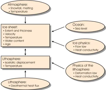
simply reset to the melting point as done in other ice sheet models. SICOPO-LIS has been benchmarked in a number of international ice sheet modeling inter-comparison projects such as EISMINT (European Ice Sheet Modeling INi-Tiative) and ISMIP-HEINO (Ice Sheet Model Intercomparison Project - Hein-rich Event INtercOmparison) [18, 27, 26, 42]. It provides the time-dependent extent, thickness, velocity, temperature, water content and age for grounded ice sheets in response to external forcing, such as air-temperature, snowfall, geothermal heat flux, sea level etc., see figure 6. Furthermore, isostatic effects due to ice load are modeled by the Elastic-Lithosphere-Relaxing-Asthenosphere (ELRA) or Local-Lithosphere-Relaxing-Asthenosphere (LLRA) approach [13]. Apart from the isostatic adjustment, heat conduction in the lithosphere is the only other lithospheric process accounted for. Heat conduction results in a thermal effect at the base of ice masses and enters the simulations through the geothermal heat flux with its globally averaged value of 55 · 10−3_Wm−2_{. More}

detailed information concerning SICOPOLIS can be found in the doctoral thesis by Greve [11] and at the SICOPOLIS-website [41].

Figure 6: Flowchart showing the general structure of SICOPOLIS. Ovals contain model input and squares contain prognostic model components. Figure by Greve, with kind permission.

For every time-step SICOPOLIS computes (in order) temperature, stresses, velocity and ice surface evolution. The general structure of SICOPOLIS will be kept when adding the second order equations. In each time step, the zeroth order solution will be computed and after this the second order solution is computed. This order is necessary since the second order solution is dependent on the zeroth order solution. The algorithm is illustrated (somewhat simplified) in the flowchart in figure 7. The updated, second order version of SICOPOLIS will from now on be called SOSIA-SICOPOLIS.

(20)

Figure 7: The over-all structure of SICOPOLIS, including higher order contributions. Red rectangles show files with zeroth order contributions, green rectangles show first order contributions and blue rectangles show second order contributions. Solid lines show files that are implemented in the code, and dashed lines are for files that should be included in the future. In some rectangles, the quantities computed in the file and the equations determining this quantity is given. The FOSIA and SOSIA are essentially given by the same equations as the in the SIA, only in first and second order instead of zeroth order.

(21)

4.2 Vertical Integration

To simplify computations, some SIA-equations are integrated in the vertical direction before implementation in SICOPOLIS. This is favorable when com-puting a variable that is differentiated in the vertical direction in the equation that determines it. If the equation would be implemented in the code without preceding integration, a linear system would have to be solved, which is com-putationally costly. In the SIA vertical integration is applied when computing shear stresses and horizontal velocities. This will be the case also in the SOSIA-equations (see section 4.6). To illustrate, let us use the zeroth order momentum balance in the x-direction as an example. In zeroth order it is used to compute the shear stress ˜tE

xz(0):

−∂ ˜_{∂ ˜}p(0)_x +∂˜t

E xz(0)

∂ ˜z = 0. (36)

To solve this for ˜tE

xz(0), the equation is integrated in the vertical direction. For

stresses there is a boundary condition at the ice surface (the ice surface is as-sumed stress-free), but not at the ice base. Equation (36) is therefore integrated from an arbitrary z-value to the ice surface. In the case of computing velocities, where there is a boundary condition at the base and not at the ice surface, the equation is integrated from the base to an arbitrary z-value instead. Integration gives: ˜ tExz(0)= ( h˜ ˜ z ∂ ˜p(0) ∂ ˜x d˜z. (37)

It can be shown, using the momentum balance in z-direction, that

˜

p(0)(x, y, z, t) = ˜h(0)(x, y, t)− ˜z. (38)

Inserting this in equation (37) gives

˜ tE_xz(0)(., z) = (˜z_{− ˜h}(0)) ∂˜h(0) ∂ ˜x =−(˜h(0)− ˜z) ∂˜h(0) ∂ ˜x . (39)

This equation gives a simple formula for the zeroth order shear stress which is easy to implement, in contrast to equation (36).

4.3 Coordinate Transformation

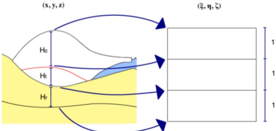
To ensure that the grid points coincide with the boundaries (i.e. the surface of the ice, the upper- and underside of the lithosphere and the CTS) the vertical z-coordinate in each domain (lithosphere, temperate ice and cold ice) are mapped to the interval [0, 1]. The transformation is from (x, y, z) to (ξ, η, ζ), where the mapping from (x, y) to (ξ, η) introduces nothing new. In SICOPOLIS, the grid is thus equidistant in the horizontal but not in the vertical direction. The transformation is referred to as the σ-transformation and is illustrated in figure

(22)

Figure 8: The cold ice, the temperate ice and the lithosphere are transformed such that each domain is of thickness one. Hc is the thickness of the cold ice layer, Ht is

the thickness of the temperate ice layer and Hr is the thickness of the lithosphere.

At the CTS, the ice/water goes through a phase change (a Stefan-type prob-lem) and a high resolution is thus needed in this area. For this purpose, an ex-ponential stretching z to ζ is introduced. When polythermal mode is switched off the position of the CTS (denoted by zm, see figure 5) will be equal to the

position of the base. The transformations are given (for completeness) for the cold ice layer, the temperate ice layer and the bedrock (subscripts c, t and e) and follow as [13]: x = ξc, y = ηc, z_{− z}m Hc = eaζc_{− 1} ea_{− 1} =: ε(ζc), (40) x = ξt, y = ηt, z− b Ht = ζt, (41) x = ξr, y = ηr, z− br Hr = ζr, (42)

where the stretching parameter a is often set to 2. Above, zm is the position of

the CTS, b is the position of the ice base and bris the position of the boundary

between the lithosphere and the asthenosphere, see figure 5. Hcis the thickness

of the cold ice layer (Hc= h−zm), Htis the thickness of the temperate ice layer

(Ht= zm− b) and Hr is the thickness of the lithosphere (Hr= b− br). Since

only cold ice is considered in this work, the transformations in temperate ice and in the lithosphere are omitted in the following. The σ-transformation must be considered when integrating in the vertical direction and when differentiating. With the abbreviation

(23)

the following rules apply for cold ice: ∂ ∂m (44) = ∂ ∂µ− 1 Hcaeaζc # (ea− 1)∂z_∂mm + (eaζc_{− 1)}∂Hc ∂m $ ∂ ∂ζc =: Dm, ∂ ∂z = ea − 1 Hcaeaζc ∂ ∂ζc =: Dz, (45) ( (_•)dz!= ( (_•)Hcae aζc ea_{− 1} dζ ! c =: IntZ(•). (46)

Dm, Dz and IntZ have been introduced to represent the transformed

differen-tial/integral operators. Remember that if polythermal mode in SICOPOLIS is switched off, zm equals b.

When only the SIA is considered, the order in which the perturbation expan-sion and the σ-transformation are performed does not matter, and in practice, the σ-transformation is applied first. However, in higher order approximations, the two operations are not commutative any longer as the σ- transformation includes the thicknesses Hc, Htand Hr, the position of the ice base, b, the

posi-tion of the CTS, zb, and the position of the ice surface, h. These variables also

need to be extended in power series of ( in the same manner as in section 2.3.2, and when going to higher orders, actually have to be applied before carrying out the perturbation expansion and splitting the equations into the zeroth, first and second order equations. The higher order equations derived by Baral [3] thus need adjustment to be valid for the grid used in SICOPOLIS. This is done below. Note that the σ-transformation introduces nothing new in the scaling of the equations. The perturbation expansion of the σ-transformation up to second order (for cold ice) follows as:

ε(ζc) = (47) = z− zm(0)− (zm(1)− ( 2_z m(2)− . . . Hc(0)+ (Hc(1)+ (2Hc(2)+ . . . = z− zm(0) Hc(0) − ( 1 Hc(0) #_H c(1) Hc(0) (z_{− z}m(0)) + zm(1) $

(24)

+ (2 1 Hc(0) # zm(1) Hc(1) Hc(0) − (z − zm(0) )Hc(2) Hc(0)− zm(2) $ +_{· · · =} = ε(ζc))(0)+ ((ε(ζc))(1)+ (2(ε(ζc))(2)+ . . . ,

where the denominator was expanded using Maclaurin series. These equations generalize the equations given in Greve and Blatter, 2009 [13]. The zeroth order transformation is structurally in the same form as the exact transformation. Applying the σ-transformation before the perturbation expansion will hence not affect the zeroth order equations but will add terms to the higher order equations. The perturbation expansion of the transformation rules for cold ice, needed when differentiating and integrating, follow as:

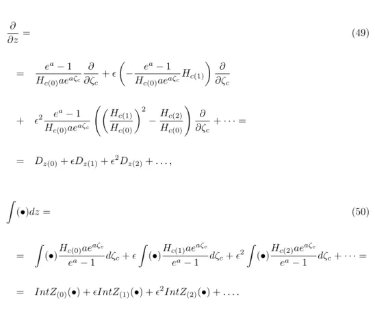
∂ ∂m= (48) = ∂ ∂µ− 1 Hc(0)aeaζc # (ea− 1)∂z_∂mm(0) + (eaζc_{− 1)}∂Hc(0) ∂m $ ∂ ∂ζc + ( 1 Hc(0)aeaζc # (ea_{− 1)} # −∂z_∂mm(1)+Hc(1) Hc(0) ∂zm(1) ∂m $ + (eaζc_{− 1)} # −∂H_∂mc(1)+Hc(1) Hc(0) ∂Hc(0) ∂m $$ ∂ ∂ζc + (2 1 Hc(0)aeaζc # (ea_{− 1)} # −∂z_∂mm(2) +Hc(1) Hc(0) ∂zm(1) ∂m + ) Hc(2) Hc(0) + #_H c(1) Hc(0) $2* ∂zm(0) ∂m * + (eaζc − 1) # −∂H_∂mc(2)+Hc(1) Hc(0) ∂Hc(1) ∂m + ) Hc(2) Hc(0) + #_H c(1) Hc(0) $2*_∂H c(0) ∂m ** ∂ ∂ζc +_{· · · =} = Dm(0)+ (Dm(1)+ (2Dm(2)+ . . . ,

(25)

∂ ∂z = (49) = e a − 1 Hc(0)aeaζc ∂ ∂ζc + ( # − e a − 1 Hc(0)aeaζc Hc(1) $ _∂ ∂ζc + (2 e a − 1 Hc(0)aeaζc )#_H c(1) Hc(0) $2 −H_Hc(2) c(0) * ∂ ∂ζc +_{· · · =} = Dz(0)+ (Dz(1)+ (2Dz(2)+ . . . , ( (_{•)dz =} (50) = ( (_•)Hc(0)ae aζc ea_{− 1} dζc+ ( ( (_•)Hc(1)ae aζc ea_{− 1} dζc+ ( 2( ₍ •)Hc(2)ae aζc ea_{− 1} dζc+· · · =

= IntZ(0)(•) + (IntZ(1)(•) + (2IntZ(2)(•) + . . . .

In second order, it is the second order boundaries that coincide with grid points, while the zeroth, and first order boundaries do no longer so. This is illustrated in figure 9 for the cold ice region. This is important to remember

Figure 9: In second order, the second order boundaries coincide with the grid but the zeroth and first order boundaries do not. Note that in this figure, for simplicity, it looks like the first and second order contributions are always positive, which is not necessarily the case.

when implementing the equations in the code. In section 4.2 the vertical in-tegration of equations was described. When integrating in second order, one needs to expand the limits of integration by perturbation expansion as well, as:

( h z f (x, y, z)dz = ( h(0)+"h(1)+"2h(2) z f (x, y, z)dz, (51)

(26)

where f is an arbitrary variable. If f is of zeroth order, there will be additional higher order terms arising from the integration, but these contain no new infor-mation. If f is of second order, the limits of integration should to stay at zeroth order in order to keep the integral of f at second order. Since the zeroth order boundaries do not coincide with the grid points, this is however not possible to implement. It is the second order boundaries that coincides with grid points, and thus the limit of integration has to be of second order. The integral will then actually include some terms of third and fourth order. This is not an issue since it actually slightly increases the accuracy of the solution; it could at most be seen as a slight inconsistency.

Since all of the higher order transformation terms include contributions from the higher order topography and ice-surface they can luckily be disregarded in this work since the equation regarding the evolution of the ice-surface is not solved for higher order here. The higher order transformation terms will however matter as this work is continued as a doctoral thesis.

4.4 Dimensional Form

In order to obtain the SIA-, FOSIA- and SOSIA-equations, all variables are scaled to dimensionless form, but in SICOPOLIS, the SIA-equations are im-plemented in dimensional form. The SOSIA-equations will therefore also be implemented in dimensional form. To obtain them, the relations given in sec-tion 2.3.1 are inverted. Returning to the momentum balance in the x-direcsec-tion as an example, we need the following relations:

˜ x = x [L], ˜ z = z [H], (52) ˜ p = p ρg[H], ˜ tE xz = tE xz (ρg[H],

which can be used to deduce equation (39) in dimensional form:

tExz(0)=−ρg(h(0)− z)

∂h(0)

∂x . (53)

The difference between equation (53) in dimensional form and equation (36) in dimensionless form is a factor of ρg. This factor appears when deducing the remaining SIA-equations as well. In rescaling the SOSIA-equations to dimen-sional form, not only will a factor of ρg appear, but also one of 1

"2. When adding

together the SIA, (FOSIA) and SOSIA contributions this factor of 1

"2 and the

factor of (2 _{arising from the power series expansion will cancel each other out,}

and the final solution will not explicitly depend on (.

4.5 Discretization

The model is discretized using finite differences with an equidistant, staggered grid in the σ- coordinates. The domain is a rectangle containing the whole ice

(27)

sheet and the surrounding ocean. In space and time, the discretization is

x(i) = ξc(i) = ξt(i) = ξr(i) = x0+ i∆x, (i = 0 . . . imax),

y(j) = ηc(j) = ηt(j) = ηr(j) = y0+ j∆y, (j = 0 . . . jmax),

ζc(kc) = kc/kc,max, (kc= 0 . . . kc,max),

ζc(kt) = kt/kt,max, (kt= 0 . . . kt,max), (54)

ζc(kr) = kr/kr,max, (kr= 0 . . . kr,max),

t(n) = τc(n) = τt(n) = τr(n) = t0+ n∆t, (n = 0 . . . nmax),

t(ñ) = τc(˜n) = τt(˜n) = τr(ñ) = t0+ ˜n∆˜t, (˜n = 0 . . . ñmax).

The parameters kc,max, kt,max and kr,max are held fixed during a simulation,

and since the thickness of the lithosphere, the temperate layer and the cold ice layer always are one in the transformed coordinates, ∆ζc,t,r = _k_c,t,r,max1 will

also be a fixed value even though the boundary surfaces are evolving in time. Since different processes are happening under different time scales, two different time steps appear, ∆˜t for computation of temperature, water content, ice age

and CTS position, and ∆t for all other computations. ∆˜t is a multiple of ∆t

[11]. For stability reasons the velocities, the horizontal volume fluxes, vertical shear stresses and the horizontal derivatives of bedrock topography, ice-surface topography, CTS, cold and temperate ice layer thickness etc. are defined in between the grid points. All other quantities are defined at grid points. When a quantity is needed in a point where it is not defined, linear interpolation is used.

Derivatives are discretized using central differences, which are second order accurate. At the horizontal boundaries there are no boundary conditions. Here, one-sided differences are used, which are first order accurate. If the derivative of a variable defined in between grid points is needed at grid points, the boundary points are not defined. To solve this problem the boundary points are defined by copying values from inner points to boundary points (for the benchmark experiments described in section 5.2, periodic boundary conditions are applied instead). Since the ice flows outwards to the horizontal edges, the reduction in accuracy at the boundaries is assumed not to affect the solution. When computing integrals numerically, the trapezoidal rule is used if the integrand and the integral is defined at the same points. If the integrand and the integral are defined at different points (one in between grid points and one at grid points), the mid point rule is used instead. These to cases are equivalent.

4.6 Implemented Equations

In the doctoral thesis by Baral [3], expressions for the second order pressure and shear stresses are given in dimensional form in Cartesian coordinates. Expres-sions for the velocity are however not given. In this section the derivation of the pressure and vertical shear stress is briefly described and the σ-transformation is applied to these formulas. Expressions for the velocity are derived and trans-formed to σ-coordinates. The zeroth order normal deviatoric stresses and HP shear stress are also given, since they need to be implemented into SICOPOLIS in order to compute the second order pressure and vertical shear stress. For

(28)

brevity of presentation the fact that the coordinate transformation can be ap-plied after the perturbation expansion when higher order topography terms are zero is exploited.

4.6.1 Zeroth Order Stresses

The zeroth order normal deviatoric stresses txx(0), tyy(0) and tzz(0) and the HP

shear stress txy(0)that are needed in SOSIA-SICOPOLIS stresses are obtained

from the zeroth order stress-strain rate relation:

˜ tE_xx(0) = 1 KE Ã ˜f (˜σ(0)) ∂˜vx(0) ∂ ˜x , (55) ˜ tEyy(0) = 1 KE Ã ˜f (˜σ(0)) ∂˜vy(0) ∂ ˜y , (56) ˜ tEzz(0) = 1 KE Ã ˜f (˜σ(0)) ∂˜vz(0) ∂ ˜z , (57) ˜ tE xy(0) = 1 2KE Ã ˜f (˜σ(0)) #_∂˜_v x(0) ∂ ˜y + ∂˜vy(0) ∂ ˜x $ . (58)

In dimensional form these equations are the same, except for the constant _K which only occurs in the scaled equations. For the creep response function

f (σ(0)) a finite viscosity law is used in the form mentioned in section 2.3.3.

Coordinate transformation and scaling back to dimensional form gives:

txx(0) = 1 EA(T! (0))f (σ(0)) #_∂v x(0) ∂ξ (59) − _H 1 caeaζc # (ea− 1)∂z_∂ξm +!eaζc_{− 1}" ∂Hc ∂ξ $_∂v x(0) ∂ζc $ , tyy(0) = 1 EA(T! (0))f (σ(0)) #_∂v y(0) ∂η (60) − _H 1 caeaζc # (ea − 1)∂z_∂ηm +!eaζc − 1" ∂H_∂ηc $_∂v y(0) ∂ζc $ ,

(29)

tzz(0) = 1 EA(T! (0))f (σ(0)) ea − 1 Hcaeaζc ∂vz(0) ∂ζc , (61) txy(0) = 1 2EA(T! (0))f (σ(0)) #_∂v x(0) ∂η + ∂vy(0) ∂ξ (62) − _H 1 caeaζc # (ea − 1)∂z_∂ηm +!eaζc − 1" ∂H_∂ηc $_∂v x(0) ∂ζc − _H 1 caeaζc # (ea − 1)∂z_∂ξm +!eaζc − 1" ∂H_∂ξc $_∂v y(0) ∂ζc $ .

These stresses are included in the equations that determine the second order pressure and the second order shear stress. For this purpose it is convenient to define the stresses at grid points.

4.6.2 Pressure

The second order pressure is given by the z-component of the momentum bal-ance together with the second order boundary condition for the stress at the ice surface. The second order equation for this was given in section 2.3.1 as

0 = ₋∂ ˜p(2) ∂ ˜z + ∂˜tE xz(0) ∂ ˜x + ∂˜tE yz(0) ∂ ˜y + ∂˜tE zz(0) ∂ ˜z , (63)

and the second order boundary condition is

∂ ˜p(0)(., h(0)) ∂ ˜z ˜h(2)+ 1 2 ∂2_p_˜ (0)(., ˜h(0)) ∂ ˜z2 ˜h 2 (1) (64) + ∂ ˜p(1)(., ˜h(0)) ∂ ˜z ˜h(1)+ ˜p(2)(., ˜h(0))− ˜tzz(0)(., ˜h(0)) = = _−˜h(2)+ ˜p(2)(., ˜h(0))− ˜tzz(0)(., ˜h(0)) = 0.

Integrating equation (63) from an arbitrary elevation to the ice surface and inserting the boundary condition (64) and the expressions for the zeroth order stresses (see e.g. Baral et al. 2001 [4]), gives the formula for the second order pressure,

(30)

˜ p(2)= 1 2 + ˜ h(0)− ˜z ,2 ∇2H˜h(0) (65) + +˜h(0)− ˜z, ---∇H˜h(0) --2+ ˜h(2)+ ˜tzz(0),

which can be compared to the zeroth order pressure given in equation (38). Co-ordinate transformation and scaling back to dimensional form gives for equation (65): p(2)= 1 2 ρg (2 ! Hc(0)(ε(ζc)− 1)" 2 ∇2 Hh(0) (66) − ρg₍2 ! Hc(0)(ε(ζc)− 1)" --∇Hh(0) --2 + ρgh(2)+ 1 (2tzz(0).

In this work, the topography computation is not extended to second order, so the term ρgh(2) is not implemented. The pressure is defined at grid points.

4.6.3 Vertical Shear Stresses

The second order vertical shear stress terms txz(2)and tyz(2)are needed for the

computation of second order velocities. The equation for tyz(2) is in the same

form as for txz(2), and in this section only the derivation of the second order

vertical shear stress in x-direction, txz(2), is presented. This stress is given by

the balance of linear momentum in x-direction,

0 =−∂ ˜_{∂ ˜}p(2)_x +∂˜t E xz(2) ∂ ˜z + ∂˜tE xx(0) ∂ ˜x + ∂˜tE xy(0) ∂ ˜y , (67)

and the boundary condition for the stress tensor at the ice surface,

˜ tExz(2)(., ˜h(0)) =− ∂˜h(0) ∂ ˜x ˜h(2)− ∂˜h(1) ∂ ˜x ˜h(1)= (68) = ₋+˜tE zz(0)(., ˜h(0))− ˜tExx(0)(., ˜h(0)) , ∂˜h(0) ∂ ˜x + ˜t E xy(0)(., ˜h(0)) ∂˜h(0) ∂ ˜x .

(31)

Integrating equation (67) from an arbitrary elevation to the ice surface using the Leibniz rule, inserting the boundary condition and the expression for the second order pressure gives:

˜ txz(2)= (69) = −_{∂ ˜}∂_x # −1₆(˜z− ˜h(0))3∇2_H˜˜h(0)+ 1 2 + ˜ z− ˜h(0) ,2- --∇H˜h(0) --2 $ − ∂˜h_{∂ ˜}_x(0)˜h(2)− ∂˜h(1) ∂ ˜x ˜h(1) − ∂˜h_{∂ ˜}_x(2)(˜h(0)− ˜z) − _{∂ ˜}∂_x ( ˜_h₍₀₎ ˜ z ˜ tzz(0)d˜z!+ ∂ ∂ ˜x ( ˜_h₍₀₎ ˜ z ˜ txx(0)d˜z! + ∂ ∂ ˜y ( _h˜₍₀₎ ˜ z ˜ txy(0)d˜z!,

which can be compared to the expression for the zeroth order vertical shear stress in the x-direction, given in (39). The higher order topography terms

∂˜h(0)

∂ ˜x h˜(2), ∂˜h(1)

∂ ˜x h˜(1) and ∂˜h(2)

∂ ˜x (˜h(0)− ˜z) are zero since the equation regarding the

evolution of the ice surface is not solved, and will in the following be omitted for brevity of presentation. In σ-coordinates and dimensional form, equation (69) is: txz(2)= (70) = − # ∂ ∂ξ − 1 Hcaeaζc # (ea− 1)∂z_∂ξm+!eaζc_{− 1}" ∂Hc ∂ξ $ ∂ ∂ζc $ # −1₆!Hc(0)ε(ζc)− 1" 3 ∇2 Hh(0)+ 1 2 ! Hc(0)ε(ζc)− 1" 2 --∇Hh(0) --2$ + # ∂ ∂ξ − 1 Hcaeaζc # (ea− 1)∂z_∂ξm+!eaζc_{− 1}" ∂Hc ∂ξ $ ∂ ∂ζc $ ( h(0) ζc Hcaeaζ ! c ea_{− 1} ! txx(0)− tzz(0) " dζ_c!

(32)

+ # _∂ ∂η − 1 Hcaeaζc # (ea_{− 1)}∂zm ∂η + ! eaζc − 1" ∂H_∂ηc $ _∂ ∂ζc $ ( h(0) ζc Hcaeaζ ! c ea_{− 1} txy(0)dζc!.

The vertical shear stresses are defined in between grid points, i.e. txz(2) is

defined at (i + 1/2, j, kc) and tyz(2) at (i, j + 1/2, kc). The integrals are defined

at grid points, and the derivatives of the integrals are defined in between grid points. The integrals are computed using the trapezoidal rule.

4.6.4 Horizontal Velocities

The horizontal velocities are computed from the stress-strain rate relationship together with the sliding condition at the ice base. The expression for the second order velocity in x-direction, vx(2) is in the same for as the expression for the

second order velocity in y-direction and only the derivation of vx is presented

here. The second order stress- strain rate relation that gives vxis

∂˜vx(2) ∂ ˜z + ∂˜vz(0) ∂ ˜x = (71) = 2_K˜txz(0) ) ˜ A(θ₍₀₎! )d ˜f (˜σ(0)) d˜σ σ˜(2)+ 1 2A(θ˜ ! (0)) d2_{f (˜}_˜_σ (0)) d˜σ2 ˜σ 2 (1) + d ˜A(θ ! (0)) d˜θ! f (˜˜σ(0))˜θ ! (2)+ d ˜A(˜θ! (0)) d˜θ! d ˜f (˜σ(0)) d˜σ θ˜ ! (1)σ˜(1)+ 1 2 d2 d˜θ!2f (˜˜σ(0))˜θ !₂ (1) * + 2_K˜txz(2)A(˜˜ θ!(0)) ˜f (˜σ(0)) + 2K˜txz(1) ) ˜ A(˜θ(0)! ) d ˜f (˜σ(0)) d˜σ σ˜(1)+ d ˜A(˜θ! (0)) d˜θ! f (˜˜σ(0))˜θ ! (1) * , where d ˜f (˜σ(0)) d˜σ = d˜σ2 (0) d˜σ = 2˜σ(0) d˜σ(0) d˜σ = (72) = 2˜σ(0) d(˜σ_{− (˜σ}(1)− (2σ˜(2)− . . . ) d˜σ ≈ 2˜σ(0).

(33)

Note that this holds even if a constant is added to the ˜f (˜σ(0)) in order to avoid

singularities. The termd ˜A(˜θ(0)! )

d˜θ! f (˜˜σ(0))˜θ!(2)in equation (71) will not be considered

because the temperature is held constant in this work. The necessary boundary condition is the second order sliding condition, which follows as

∂(˜vsl)x(0)(., ˜b(0)) ∂ ˜z ˜b(2)+ 1 2 ∂2_(˜_v sl)x(0)(., ˜b(0)) ∂ ˜z2 ˜b 2 (1) (73) + ∂(˜vsl)x(1)(., ˜b(0)) ∂ ˜z ˜b(1)+ (˜vsl)x(2)(., ˜b(0)) =−F C(. . . ),

where ˜vsl)x(0) denotes the difference between the velocity in the ice and the

velocity in the lithosphere. Since the sliding coefficient C is set to zero in this work, the terms within the parenthesis are omitted. Omitting all higher order terms of the topography b and considering the velocity in the lithosphere to be zero, we have that:

(˜vsl)x(2)(., ˜b(0)) = 0, (74)

and since the horizontal velocities in the lithosphere are zero, the basal velocity is given by

˜

vx(2)(., ˜b(0)) = 0. (75)

The horizontal velocity in the ice is given by integrating equation (71) from the base to an arbitrary elevation using the Leibniz rule. Considering equation (72) and the sliding condition, and omitting all higher order topography terms gives the horizontal velocity gives

˜ vx(2)=− ∂ ∂ ˜x ( z˜ ˜_b₍₀₎v˜z(0)d˜z− ∂˜b(0) ∂x v˜z(0)(., ˜b(0)) (76) + 4K ( ˜z ˜ b(0) ˜ txz(0)A(˜˜ θ!(0))˜σ(0)σ˜(2)d˜z + 2K ( z˜ ˜ b(0) ˜ txz(2)A(˜˜ θ!(0)) ˜f (˜σ(0))d˜z!.