An Investigation and Development of Three Estimators of Inverse Covariance Matrices With Applications to the Mahalanobis Distance

An Investigation and Development of

Three Estimators of Inverse

Covari-ance Matrices with Applications to

the Mahalanobis Distance

H.E.T. HOLGERSSON AND PETER S. KARLSSON

Jönköping International Business School Jönköping University JIBS Working Papers No. 2010-11

1

An Investigation and Development of Three Estimators of Inverse

Covariance Matrices with Applications to the Mahalanobis Distance

H.E.T. Holgersson Peter S. Karlsson

Jönköping University Jönköping University

SE-551 11 Jönköping SE-551 11 Jönköping

Sweden Sweden

Abstract. This paper treats the problem of estimating the inverse covariance matrix in an increasing dimension context. Specifically, three ridge-type estimators are considered, of which two new are proposed by the authors and one has been considered previously. Risk functions for deciding an appropriate value of the ridge coefficient are developed and the finite sample properties of the estimators are investigated in a Monte Carlo simulation. Moreover, risk functions for the Mahalanobis distance are derived which, in turn, leads to three new estimators which has not been considered previously.

Keywords. Ridge estimators, inverse covariance matrix, increasing dimension, Mahalanobis distance, adaptive estimator.

2 I Introduction

Statistical analyses frequently involve co-variations between a large number of variables, e.g. cluster analysis, principal component analysis or discriminant analysis which requires estimators of covariance matrix. The sampling properties of such estimators, however, are known to be poor if the dimension of the statistic (p) is comparable to the sample size (n). Moreover, in cases when p grows asymptotically with n it frequently happens that the statistic does not converge to its true parameter – a well-known example is the non-convergence of the sample periodigram. While such increasing dimension asymptotics (IDA) have long been considered in time series contexts, e.g. White and Domowitz (1984), Newey and West (1987), they have been given less attention in the cross-section context. In 1967, however, Marchenko and Pastur published a pioneering paper on the convergence of spectral functions of sample covariance matrixes for zero-mean and unit-variance variables, where p and n were allowed to grow simultaneously in such a way that their quotient limits a constant. Later on, a number of important contributions were made to IDA, many of which involved relaxing the moment restrictions. Some important references include Jonsson (1982), Yin, Bai and Krishnaiah (1988) and Silverstein and Bai (1995) who derived limits for the eigenvalues. Girko (1975, 1990) used spectral theory (basically, traces of resolvents of random matrixes) to derive more general IDA properties of eigenvalues and determinants of covariance matrixes. Many of these results were also refined and put in a more applied context. In particular, Serdobolskii (1985, 2000, 2008) used spectral theory to derive IDA properties of the inverse covariance matrix which in turn was used in problems concerning discriminant analysis, estimation of high-dimensional expectation vectors and regression analysis. These contributions involve estimators which, unlike traditional estimators, have risk functions that are bounded even when the dimension of the parameter grows asymptotically and they therefore provide highly interesting alternatives to traditional methods. Little, however, is known about these estimators’ behavior in finite, given combinations of n and p Moreover, they are all shrinkage estimators in the sense that they depend on . a coefficient that pulls the estimator towards a certain point. For these reasons it is of great interest to investigate the proposed IDA estimators relative to traditional estimators and other shrinkage estimators. Most of the research of ridge estimators

3

conducted so far has focused on the search of an optimal ridge coefficient within a given family of estimators. Little is therefore known about the superiority of one family of one estimator to another. One purpose of this paper is therefore to investigate the properties of resolvent-type estimators proposed in the literature and to compare it to other shrinkage estimators of different functional form. Specifically, three types of shrinkage estimators of the inverse covariance matrix are considered: (i) the multiplicative resolvent-type estimator proposed by Girko (1995) and Serdobolskii (1985, 2000, 2008) whose finite sample properties have only been investigated for some highly restrictive cases previously, (ii) an additive resolvent-type estimator which does not seem to have been given any attention in terms of estimating inverse covariance matrices but has been frequently used in regression contexts (Hoerl and Kennard 1970a, 1970b) and (iii) a new type of shrinkage estimator that may be considered as a mixture of the first two. The IDA properties of these estimators are examined with respect to two different squared error loss functions (describing the risk of the estimators) by means of Monte Carlo simulations. Moreover, it is demonstrated that the risk function proposed by Serdobolskii (2000) for finding an optimal value of the ridge coefficient within the resolvent-type estimator may be modified to comprise the other two estimators as well, and hence that all three estimators are feasible. There is also an issue surrounding the properties of the three estimators when used within a composite statistic, since the inverse covariance matrix alone is only of partial interest. Therefore the simulations also includes the Mahalanobis distance, which is a function of the inverse covariance matrix. Furthermore, adaptive risk functions for identifying the optimal ridge coefficients with respect to the Mahalnobis distance residual sum of square are developed, and their consistencies are proved. In other words, feasible estimators are developed for estimating the Mahalanobis distance in IDA contexts. These, in turn, should be of great interest as a tool for outlier detection in IDA contexts.

4 2 Estimation of covariance matrices

A frequently used estimator of Cov

( )

X =Σ_{(p p× )} is given by

1

(

)(

)

1 , n p p n i i i − × =

∑

= − − ′ S X X X X (2.1) where

{ }

X_{i i}n₌₁ is a set of n independent observations on a p-dimensional random vector X_{( )p×1} (sometimes with a small-sample adjustment of the divisor). It is well known that S converges in probability to Σ under fairly mild moment restrictions when p is fixed and finite. Alternative estimators have also been proposed. Important references include Kubokawa and Srivastava (2003), Daniels and Kass (2001), Shäfer and Strimmer (2005). In this paper no further attention will be paid to the problem of estimating Σ , instead concentration will be on the estimation of its inverse Σ−1. An obvious estimator is given by the inverse of the standard estimator, −1

S . This estimator, however, is not well behaved if p increases with the same rate as n. For example, setting

( )

(

)

2 1 1 1 1 ˆ ˆ _, p R − =E p tr_ − − − − _   Σ Σ Σ (2.2)

where E

[ ]

⋅ is the expectation operator, tr

( )

⋅ is the trace operator of a matrix and letting _ˆ 1 1 , − ₌ − Σ S the limit in (2.2) is

( )

1 _lim

( )

1 _. p p R − R − →∞ = S S (2.3)

The function (2.3) limits infinity if p n→q−1>0 and so the standard estimator is degenerate in that case. Therefore much attention has been paid to developing better estimators of −1

Σ . One family of estimators consists of scalar transformations of the standard estimator, say Σˆ−1=

α

S−1. Such estimators are frequently referred to as Stein-type estimators or shrinkage estimators as α is usually smaller than one. While there are estimators within this family which have asymptotically bounded risk functions even for q→1, they are often of little value in cases when Σ−1 is to be used

5

in a wider context, e.g. when the statistic of main interest is a composite function

( )

1

g Σ− . This is so because scalar transformations will usually result in mappings of

the type g

(

α

Σ−1

)

=

α

g

( )

Σ−1 , or even g

(

α

Σ−1

) ( )

=g Σ−1 as in e.g. Zellners SUR models (Zellner, 1962). For this reason such estimators seem to exercise their main potential in cases when the sole purpose is to estimate Σ−1 alone, and therefore other estimators that have a wider field of usages will be considered instead. Of particular interest is an estimator defined by

Σˆ−1=Σˆ t

( ) (

= +I tS

)

−1, 0≤t. (2.4) The normalized trace of an estimator of the inverse covariance matrix in the form of the estimator (2.4), in the literature called the reolvent*, is denoted by

( )

1

( )

1

ˆ ˆ _.

h t =p trace− Σ− A key property of (2.4) is that its trace limits a fixed constant as p increases whereas p trace−1

( )

S−1 does not, as discussed above. Moreover, (2.4) also plays an important role as an estimate of _Σ−1_{, and its theoretical IDA properties}

have been investigated by Girko (1990) and Serdobolskii (1985, 2000, 2008). The key difference between _{S and} −1 _ˆ−1

Σ may be examined by their eigenvalues: let λi be the

i:th ordered eigenvalue of S. Then the i:th eigenvalue of _{S is} −1 1

i

λ− _{while the i:th} eigenvalue of _ˆ−1

Σ is

(

1 t

λ

i

)

1.

−

+ Hence the eigenvalue of _ˆ−1

Σ , say λˆ_i−1, is always bounded above zero. The idea of ensuring that the smallest eigenvalue of an inverse quadratic form does not become too small, and hence produce estimators with large sampling variance, is not unique to resolvent-type estimators. In the early 1970s, Hoerl and Kennard (1970a, 1970b) proposed a family of ridge estimators in a context of regression analysis, though similar estimators were also proposed before that (e.g. Foster, 1961). Since estimators of regression parameters involve the inversion of a quadratic form, say

(

X X′

)

−1, these authors proposed the alternative statistic

(

)

1

tI+X X′ − for some t>0, thus ensuring that the smallest eigenvalues do not come too close to zero.

6

In terms of estimating inverse covariance matrixes, a similar estimator may be expressed by

Σɶ−1=

(

tI S+

)

−1, 0≤t. (2.5) While this kind of estimator has been extensively used in regression contexts (see e.g. Hoerl and Kennard 1970a, 1970b; Obenchain 1975, 1978; Goldstein and Smith 1974; Kibria 2003 and Gruber 1998) its potential as an estimator of the inverse covariance matrix has been given less attention in the past, especially in IDA contexts. The estimators (2.4) and (2.5) seem very alike but are actually quite different. The i:th eigenvalue of 1_{, say} 1

i

λ

− −

Σɶ ɶ , is given by

(

t+

λ

_i

)

−1 and it is readily seen that there is no functional relationship between _ˆ 1

i

λ− _and 1

i

λɶ− _{. The ridge coefficient t operates} additively in λɶ_i−1 whereas it operates multiplicatively in λˆ_i−1. A compromise between the two estimators may be obtained by

Σ−1=

(

tI+ −

( )

1 t S

)

−1, 0≤ ≤t 1. (2.6) This estimator has not been considered previously and may be thought of as a compromise between the two others since the ridge coefficient t operates in both a multiplicative and an additive way. The estimator (2.4) will hence forth be referred to as the multiplicative estimator, (2.5) will be referred to as the additive estimator while the estimator (2.6) will be referred to as the mixture estimator. When it comes to the properties of the above estimators, (2.4) has been fairly well documented analytically (Serdobolskii, 1985, 2000, 2008; Girko, 1990). The properties of the estimators (2.5) and (2.6) are not known however, and are not easy to obtain analytically, at least not within an IDA context, and are therefore subject of investigation. Estimators of inverse covariance matrixes are frequently described with respect to the loss function

(

1 1

)

1

(

1 1

)

2 1 ˆ , ˆ .

7 An alternative loss function is available from

L₂

(

Σˆ−1,Σ−1

)

= p tr−1

(

Σ Σˆ−1 −I

)

2. (2.8) Other loss functions have also been considered in the literature (e.g. Stein, 1956) but the paper will be restricted to (2.7) and (2.8). It should be noted that these loss functions are usually presented without the divisor p−1 when the dimension p is taken to be fixed, but as the argument within the trace operator is monotonically increasing in p, it is convenient to work with normalized measures. Some asymptotic properties of the estimator (2.4) with respect to (2.7) are given in Serdobolskii (1985, 2000, 2008) but little is known about the properties of (2.5) or (2.6) with respect to any of these measures, particularly for increasing dimension asymptotics. The next section is concerned with this matter.

* Functions of the kind (A−kI)−1 are usually referred to as ‘resolvents’ in the functional analysis literature (e.g. Kolmogorov and Fomin, 1957) while the same term has been used for the function

( )1

kA+I − in for instance Girko (1990) and Serdobolskii (1985, 2000).

3 Risk functions

Ridge estimators are usually connected with the problem of choosing an optimal value of the ridge coefficient (t in this case). For a double coefficient estimator of the type

α

Σˆ−1=

α

(

I+

τ

S

)

−1, α ≥0, τ ≥0, (3.1) the limit quadratic risk defined in (2.3) is the limit of

( )

_ˆ 1 1

( )

2 ₂ 1

(

1_ˆ 1

)

1

( )

_ˆ 2

p

R Σ− = p tr− Σ− − p E tr− _ Σ Σ− − _+ p E tr− _ Σ− _. (3.2)

If the type of convergence is not explicitly mentioned, then it is assumed that the convergence is in mean square. In order to establish consistent estimators of the limit risk functions of (2.5) and (2.6) we will use the following result:

8 It is known that if ~

( )

, ,

iid

i N

X 0 Σ F u_p

( )

= p−1

∑

_ip₌₁ind

(

λ

_i≤ →u

)

F u

( )

where λ_i are eigenvalues of Σ such that λ_i∈

[

c c₁, ₂

]

where c₁>0 and c₂< 3 Σ , ⋅ denotes the spectral norm of a matrix, ind

(

λ_i≤u

)

denotes an indicator function of the i:th eigenvalue, F u

( )

∈ℝ is the limit spectral distribution function and

(

0 1

)

p n→ < <y , then a statistic approximating (3.2) is available from:

Rˆ_p

( )

Σˆ−1 = Λ −ˆ₋₂ 2α

(

p−1−n−1

)

tr

(

S Σ−1ˆ−1

)

+2αp n−1 −1

( )

trΣˆ−1 2+ 2 1 _ˆ 2 , p tr α − − Σ _(3.3) where, Σˆ−1= +

(

I

τ

S

)

−1, Λ = −ˆ₋₂

(

1 pn−1

)

2 p tr−1

( )

S−2 +

(

)

(

( )

)

2 1 1 1 1

1−pn− p n− − tr S− . The result is due to (Serdobolski, 2000).

For a fixed value of α the minimum of Rˆ_p

( )

Σˆ−1 can be found numerically or graphically. An operational estimator of (2.4) is hence available by first setting

α

=1

and defining tˆ _opt. minRˆ_p τ

τ

= = and then defining an operational estimator by

Σˆˆ−1= +

(

I tˆS

)

−1. (3.4) The risk function (3.3) is actually rich enough to also provide estimates of the ridge coefficients of the other two estimators as well. To see this, note that (2.5) and (2.6) may be expressed as follows:

Σɶ−1=

(

tI S+

)

−1=

α

(

I+

τ

S

)

−1, α=_t−1_, τ =_t−1_{, (3.5)}

and

Σ−1=

(

tI+ −

( )

1 t S

)

−1=

α

(

I+

τ

S

)

−1, α =_t−1_, τ =_t−1

( )

_t−_{1 . (3.6)}

In other words, all three ridge estimators considered in the paper may be written in the form (3.1) and optimal values of the respective ridge coefficient t may be obtained

(

1 1

) ( )

1 1

ˆ _p− _n− _tr − _, −

9

from (3.3) numerically. Letting tɶ and t denote the values optimising Rˆ_p

( )

Σˆ−1 with respect to (3.5) and (3.6) respectively, the following estimators are obtained

Σɶɶ−1=

(

tɶI S+

)

−1, (3.7) and

Σ−1=

(

tI+ −

(

1 t

)

S

)

−1. (3.8) Hence three alternative estimators for the inverse covariance matrix in IDA settings are available. The finite sample properties of these estimators need to be compared with respect to different values of n and p, and also to different distributional properties of

X

. Moreover, the inverse covariance matrix is often used as a component within another statistic and optimality of Σ , for example, is not ˆˆ−1 necessarily preserved when used as an ingredient within a composite statistic. Some examples involving the inverse covariance matrixes are discriminant analysis (Pavlenko and von Rosen, 2001), Mardia’s measures of skewness and kurtosis (Mardia, 1970), Zellner’s SUR models (1962) and the Mahalanobis distance (Mahalanobis, 1936). The next section will therefore treat the latter with respect to its IDA properties.

4 The inverse covariance matrix within the Mahalanobis distance The Mahalanobis distance for a single observation is defined by

d_i2 =p−1Y Σ Y_i′ −1 _i, (4.1) where Y_i=

(

X_i−µ_X

)

and the mean value vector µ_X is assumed to be known. This measure is important in diagnostics, particularly in the search for outliers in ℝp_{. An}

estimator of (4.1) may be obtained by simply replacing the inverse covariance matrix with an appropriate estimate, say _{Σ : ˆ}−1

10

This estimator has been considered by, for instance, Mardia (1977) and Wilks (1963) who also proposed methods for explicit outlier tests, but the investigation will here be restricted to the estimator (4.2) and its properties with respect to point estimation in IDA contexts. Clearly, the stochastic properties of (4.2) will depend on the estimator

1

ˆ−

Σ and hence, if Σˆ−1=Σˆ−1

( )

t , a tool for deciding an appropriate value of the ridge coefficient t is needed. The loss function considered in Section 3 is not necessarily useful in this context. A more specialized choice, which may be thought of as the expected value of the residual sum of squares between (4.1) and (4.2), is available by

R2

( )

dˆ_i2 = p E−1 _ _i′

(

ˆ−1− −1

)

2 _i_.

Y Σ Σ Y (4.3)

To achieve an estimator of (4.3) it is convenient to expand it as follows:

( )

(

)

2 2 2 1 1 1 1 ˆ n ˆ i _i i i pR d =n E− _{ =} ′ − − − _= 

∑

Y Σ Σ Y

(

(

)

)

2 1 1 1 1 ˆ n i i i n E tr− _{ =} − − − ′ _= 

∑

Σ Σ Y Y 

(

)

(

2

)

1 1 ˆ E tr_ − − − _=  Σ Σ S 

(

) (

)

(

)

2 1 1 2 ˆ ₂ ˆ _, tr E_Σ−S_ − tr E_Σ Σ− −S_ +tr E_Σ− S_ (4.4) where 1 1 . n i i i n− ₌ ′ =

∑

S Y Y In order to derive a consistent estimate of (4.4) some simplifying lemmas, under the assumption that S is of full rank, are listed below:

(

)

1

1 1 1

ˆ ˆ ˆ

: − = −t − where − = +t − .

Lemma 1 Σ I SΣ Σ I S

Proof: Post-multiply both sides by

(

I+tS .

)

(

)

1 1 1

ˆ ˆ

: − =t− − − .

Lemma 2 Σ S I Σ

Proof: By Lemma 1, t−1

(

I Σ−ˆ−1

)

=SΣˆ−1, and since t−1

(

I Σ−ˆ−1

)

is symmetric, SΣˆ−1 is also symmetric and the Lemma follows.

(

)

1 1 1 1

ˆ ˆ

: − =t− − − −.

Lemma 3 Σ I Σ S

11

Theorem 1: Let Y be distributed as the variable of (3.3)._i Then, if p n→y, where 0< <y 1, the following convergence holds:

( )

{

( )

( )

}

{

( ) ( )

}

( )

. . 1 1 2 2 ˆ ˆ 1 2 ˆd ˆ _{2 ˆ} ˆ m s d _, R t =t− h t −p tr− Σ− − h t s t + Λ →₋ R t where h tˆ

( )

= p tr−1

(

I+tS

)

−1, s tˆ

( )

= − +1 y yh tˆ

( )

and Λ =ˆ₁

(

p−1−n−1

) ( )

tr S−1 .

Proof: By Lemma 3 it follows that

( )

(

)

1 _ˆ 1 _ˆ 1 E p tr_ − Σ− Σ− S _= E p tr t_ −1

(

−1Σˆ−1

)

_−E p tr t_ −1

(

−1Σˆ−2

)

_. In Serdobolskii (2000, 2008) it is shown that

( )

( )

. . 1 _ˆ 1 m s 1 _ˆ 1 p tr− Σ− →E p tr_ − Σ− _ and

( )

. .

(

)

1 _ˆ 2 m s 1 1_ˆ 2

p tr− Σ− →E p tr t_ − − Σ− _ which proves convergence of the first term of Rˆ₂d

( )

t . By Lemma 2 it follows that

(

( )

)

(

)

(

)

1 1 _ˆ 1 1 1 1 1 1 1_ˆ 1

. E p tr_ − Σ− Σ−S _=E p tr t_ − − Σ− _−E p tr t_ − − Σ Σ− − _

Moreover, in Serdobolskii (2008) it is shown that

( )

. . 1 1 1 ˆ m s_{E p tr}− − −   Λ → _ Σ _

( ) ( )

(

)

. .

(

)

1 1 1 1 ˆ ˆ _{th t sˆ t} m s_{E p tr}− − ˆ− −   Λ − − − → _ Σ Σ _, and E

[ ]

S =Σ1+

ο

( )

p0 K, where K is a symmetric positively semidefinite matrix consisting of residual terms with bounded norm so that E n_ −1

( )

Σ−2S _= p−1Σ Σ−2 1+

ο

( )

p0 K. Hence hˆ

( ) ( )

−t sˆ −t converges to the second term of ˆ2

( )

d R t , lim 1

(

2

)

1, n E n tr − − − →∞  Σ S = Λ and since . . 1 1 ˆ m s − − Λ → Λ the proof is complete.

Corollary 1: From the assumptions and definitions of Theorem 1,

( )

{

( )

( )

}

( ) ( )

( )

. . 1 2 1 1 1 2 2 ˆ 1 2 ˆd _, ˆ ˆ _{2 ˆ} ˆ m s d _{, ,} R

τ α τ α

= − p tr− Σ− + p tr− Σ− −

α

h −

τ

s − + Λ →

τ

₋ R

τ α

where

α

∈ℝ _{is a non-random constant and ˆ ,}

( )

1

(

(

)

1

)

_,

h t α = p−αtr I+tS −

( )

( )

(

1 1

) ( )

1 1

ˆ ˆ

ˆ , 1 , ,

s t

α

= − +y yh t

α

Λ = p− −n− tr S− and τ is a function of t determined by the inverse covariance-estimator (3.5) and (3.6).

12 Proof: Follows from the proof of (3.3).

The risk function (4.4) provides a tool for deciding an appropriate value of the ridge coefficient t for estimating the Mahalanobis distance between X and µ . Moreover, _i the estimator

(

I+tS

)

−1 within (4.2) may be replaced by the double coefficient estimator

α

(

I+tS

)

−1 which in turn encompasses all three estimators (2.4) - (2.6). Hence two alternatives to (4.2) are given by

di p 1 i 1 i, − ′ − = Y Σ Y ɶ ɶ _(4.5) di p 1 i 1 i. − ′ − = Y Σ Y (4.6)

Through Corollary 1 a tool for deciding appropriate values of the ridge coefficient for any of (4.2), (4.5) and (4.6) is available. Adhering to the notation of (3.4) – (3.6) the following feasible estimators are obtained:

dˆˆ_i =p−1Y Σ Y_i′ˆˆ−1 _i. (4.7) di p 1 i 1 i. − ′ − = Y Σ Y ɶ ɶ ɶ ɶ _(4.8) di p 1 i 1 i. − ′ − = Y Σ Y (4.9)

Thus, using any of the estimators (4.7) – (4.9) its efficiency may be evaluated with respect to (4.3) by Monte Carlo simulations. Further details are supplied in the next section.

13 5 Monte Carlo simulations

This section investigates some properties of the estimators of the inverse covariance matrix Σ−1 and the Mahalanobis distance p−1Y Σ Y_i′ −1 _i considered in the paper. In order to do this, various simulations will be conducted while varying relevant parameters. The properties of any estimator of the inverse covariance matrix will depend upon the true covariance matrix Σ . Two types of covariance matrixes are presented below which are simple to generate for any value of the dimension p:

a. Σ_{a p p,( × )}

( )

φ

=toeplitz

(

θ θ

0, 1,...,

θ

(p−1)

)

, θ <1.

b. Σ_{b p p,( × )}=P_{p p×} Λ_{p p×} P′_{p p×} where P is the eigenvector matrix of Σ and Λ is a diagonal matrix consisting of the eigenvalues of Σ . P is obtained by drawing a set of numbers

{ }

,

p ij _{i j}

P from a uniform distribution on the interval

(

1,10

)

using the ISBN number of (Rao, 1973) as random seed, and then applying the singular value decomposition to make the columns orthonormal. The eigenvalues

{

Λ₁,...,Λp

}

were drawn from a ( )

2 5

χ distribution. PΛP′ =Σ_b is then held fixed in all replicates.

The above covariance matrixes are both interesting in their own way. The multiplicative estimator (2.4) limits the identity matrix as the ridge coefficient t limits zero which is equivalent to the special case Σ_a

( )

0 , while it limits a singular matrix when φ limits unity. Moreover, the covariance matrix in (a) has its eigenvalues bounded on a finite segment, i.e. 0<λ_min≤λ_max < ∞. Since most of the methods treated in the paper assume the eigenvalues to be bounded, it is of interest to investigate covariance matrixes that violate this assumption, though in a modest sense. This is achieved by the covariance matrix in (b) since the eigenvalues obtained by a single drawing of numbers of the chi-square distribution have the property that

max

lim

p→∞

λ

= ∞. The two types of covariance matrixes therefore represent rather

different aspects of the true covariance matrix. Apart from the parametric structure of the covariance matrix, it is also important to consider transformations of the type

β

Σ֏ Σ for some scalar parameter β. Hence both the functional form of Σ and scalar transformations thereof will be considered. Another quantity of relevance is the

14

quotient q=n p/ . The multiplicative estimator has its greatest potential relative to the standard estimator S for values of q just above the value 1, say 1−1 < <q 5. Moreover, the risk function of equation (3.3) can only be considered to be a good approximation to the true risk function for large values of p . Therefore the simulations will also include a range of values of p. Carefully selected combinations of the above parameterisations should allow for investigations of the main properties of the considered estimators. The parametric setting used in the experiment in Tables 1 and 2 are listed below:

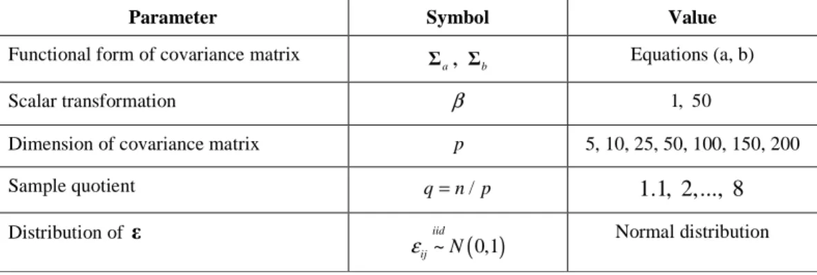
Table 1 Parameters used in simulation A (inverse covariance matrix) Parameter Symbol Value

Functional form of covariance matrix

a

Σ , Σb Equations (a, b)

Scalar transformation β 1, 50

Dimension of covariance matrix p 5, 10, 25, 50, 100, 150, 200

Sample quotient q=n p/ 1.1, 2,..., 8 Distribution of ε

_{( )}

~ 0,1 iid ij N ε Normal distribution

Table 2 Parameters used in simulation B (Mahalanobis distance)

Parameter Symbol Value

Functional form of covariance matrix Σ_a Equation (a)

Scalar transformation β 5, 500

Correlation parameter φ 0, 0.9

Dimension of covariance matrix p 5, 10,..., 50

Sample quotient q=n p/ 1.1,..., 5.5 Distribution of ε

_{( )}

( ) ( )

{

}

~ 0,1 ~ 2 2 1 2 iid ij iid ij N Exp ε ε − Normal distribution Exponential distribution

The variables used to estimate the inverse covariance matrixes are defined by

( ) ( )

(

p p p n

)

β _{× ×}

′ = +

X L ε where LL′ =Σ . The matrix Σ is held constant in all replications while a new ε is drawn in each replicate. For each combination of parameters 10 000 replicates were used.

15

A. Estimators of inverse covariance matrixes

In order to make the simulations easier to interpret the loss function of each ridge estimator has been divided with the corresponding loss for the standard estimator, e.g.

( )

1

( )

1

1 ˆ 1

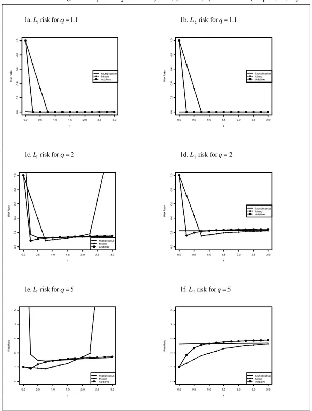
L Σ− L S− . The ridge coefficient of the mixture estimator ranges between zero and one, but is in the below graphs scaled to fit in the same graphs as the other estimators. Figures 1-2 present the risk of the three estimators (2.4), (2.5) and (2.6) when p=150 and q increase vertically (between rows of graphs). In Figure 1 all three ridge estimators dominate _S−1 _{for all values of the ridge coefficient t when}

1.1 q= (the quotients being uniformly below 1). For q=5, however, it is seen that the ridge estimators are inferior to the standard estimators for nearly all values of the ridge coefficient. In particular, the multiplicative estimator and the mixture estimator may perform drastically worse than _{S for poor choices of t. In comparison of Figure 1} −1

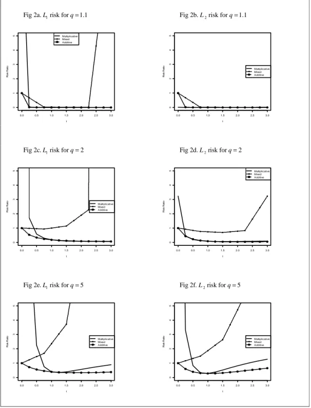
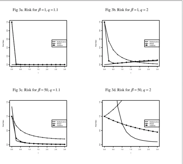
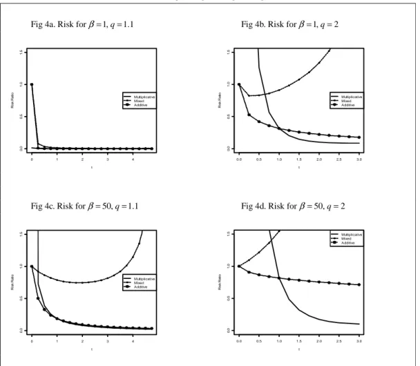
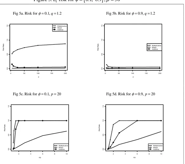
and 2 it is seen that the higher value of β leads to higher relative risk for the multiplicative and mixture estimator respectively while the risk of the additive estimator actually decreases by this change. The difference between the three estimators generally becomes more accentuated for high values of β. It is also interesting to compare the properties of the estimators with respect to the two loss functions (left vs. right column) in that good properties with respect to L₁ does not necessarily hold for L . For example, the difference between Figures 1e and 1f is ₂ notable. Moving on to the graphs within Figure 3, the effect of q is compared horizontally and the value of β vertically. Again it is seen that the ridge estimators possess their greatest potential for low values of q and that the difference between the three estimators becomes accentuated when β increases. In Figure 4 the performance of the estimators are investigated for a covariance matrix of type Σ_b as defined on p. 13. The ridge estimators may excel at estimating the inverse covariance matrix as seen from this figure, but, at the same time, they may also perform considerably worse than the standard estimator for inappropriately chosen values of t. Hence it is of great importance to examine the properties of the estimators when the ridge coefficient is determined from data. Figure 5 therefore concerns the adaptive two-stage estimators, i.e. when the value of t has been obtained from (3.3). From these graphs it is evident that the multiplicative and the additive ridge estimators perform very well for values

16

of q below 6, though high values of φ (= high covariances) deteriorate the relative performance. The mixture estimator is uniformly inferior to the other two, at least for the setting considered here. It should also be stressed that the estimator S is (for −1 normal distribution and fixed value of p) well known to asymptotically limit the maximum likelihood estimator of Σ−1 (Anderson, 2003). Hence it will be asymptotically efficient and outperform other estimators as the quotient q increases, i.e., an estimator should optimally limit S−1when the quotient between n and p grows. The mixture and the additive estimator coincide with S for a specific value of the −1 ridge coefficient (t=0) which indeed is seen to happen asymptotically as q grows (Figures 5c-5d). From this point of view, these two estimators should be considered just as useful as the multiplicative estimator even though the latter is frequently superior in the settings considered here.

17

{

}

1 2

Figure 1. and L L risk for β =1, p=150, φ=0.9 andq= 1.1, 2, 5 1a. risk for L1 q=1.1 1b. L2 risk for q=1.1

1c. risk for L1 q=2 1d. L2 risk for q=2

1e. risk for L1 q=5 1f. L2 risk for q=5

0.0 0.5 1.0 1.5 2.0 2.5 3.0 0 .0 0 .2 0 .4 0 .6 0 .8 1 .0 t R is k R a ti o Multiplicative Mixed Additive 0.0 0.5 1.0 1.5 2.0 2.5 3.0 0 .0 0 .2 0 .4 0 .6 0 .8 1 .0 t R is k R a ti o Multiplicative Mixed Additive 0.0 0.5 1.0 1.5 2.0 2.5 3.0 0 .0 0 .2 0 .4 0 .6 0 .8 1 .0 t R is k R a ti o Multiplicative Mixed Additive 0.0 0.5 1.0 1.5 2.0 2.5 3.0 0 .0 0 .2 0 .4 0 .6 0 .8 1 .0 t R is k R a ti o Multiplicative Mixed Additive 0.0 0.5 1.0 1.5 2.0 2.5 3.0 0 1 2 3 4 5 t R is k R a ti o Multiplicative Mixed Additive 0.0 0.5 1.0 1.5 2.0 2.5 3.0 0 1 2 3 4 5 t R is k R a ti o Multiplicative Mixed Additive

18

{

}

1 2

Figure 2. and L L risk for β =50,p=150, φ =0.9 andq= 1.1, 2, 5 Fig 2a. risk for L1 q=1.1 Fig 2b. L2 risk for q=1.1

Fig 2c. risk for L1 q=2 Fig 2d. L2 risk for q=2

Fig 2e. risk for L1 q=5 Fig 2f. L2 risk for q=5

0.0 0.5 1.0 1.5 2.0 2.5 3.0 0 1 2 3 4 5 t R is k R a ti o Multiplicative Mixed Additive 0.0 0.5 1.0 1.5 2.0 2.5 3.0 0 1 2 3 4 5 t R is k R a ti o Multiplicative Mixed Additive 0.0 0.5 1.0 1.5 2.0 2.5 3.0 0 1 2 3 4 5 t R is k R a ti o Multiplicative Mixed Additive 0.0 0.5 1.0 1.5 2.0 2.5 3.0 0 1 2 3 4 5 t R is k R a ti o Multiplicative Mixed Additive 0.0 0.5 1.0 1.5 2.0 2.5 3.0 0 1 2 3 4 5 t R is k R a ti o Multiplicative Mixed Additive 0.0 0.5 1.0 1.5 2.0 2.5 3.0 0 1 2 3 4 5 t R is k R a ti o Multiplicative Mixed Additive

19

{

}

{

}

1

Figure 3. risk for L β = 1, 50 ,p=150, φ=0 andq= 1.1, 2 Fig 3a. Risk for β=1,q=1.1 Fig 3b. Risk for β=1,q=2

Fig 3c. Risk for β=50,q=1.1 Fig 3d. Risk for β=50,q=2

0.0 0.5 1.0 1.5 2.0 2.5 3.0 0 .0 0 .2 0 .4 0 .6 0 .8 1 .0 t R is k R a ti o Multiplicative Mixed Additive 0.0 0.5 1.0 1.5 2.0 2.5 3.0 0 .0 0 .2 0 .4 0 .6 0 .8 1 .0 t R is k R a ti o Multiplicative Mixed Additive 0.0 0.5 1.0 1.5 2.0 2.5 3.0 0 .0 0 .5 1 .0 1 .5 t R is k R a ti o Multiplicative Mixed Additive 0.0 0.5 1.0 1.5 2.0 2.5 3.0 0 .0 0 .5 1 .0 1 .5 t R is k R a ti o Multiplicative Mixed Additive

20

{

}

{

}

1

Figure 4. risk for L Σ_b, β = 1, 50 ,q= 1.1, 2

Fig 4a. Risk for β=1,q=1.1 Fig 4b. Risk for β=1,q=2

Fig 4c. Risk for β=50,q=1.1 Fig 4d. Risk for β=50,q=2

0 1 2 3 4 0 .0 0 .5 1 .0 1 .5 t R is k R a ti o Multiplicative Mixed Additive 0.0 0.5 1.0 1.5 2.0 2.5 3.0 0 .0 0 .5 1 .0 1 .5 t R is k R a ti o Multiplicative Mixed Additive 0 1 2 3 4 0 .0 0 .5 1 .0 1 .5 t R is k R a ti o Multiplicative Mixed Additive 0.0 0.5 1.0 1.5 2.0 2.5 3.0 0 .0 0 .5 1 .0 1 .5 t R is k R a ti o Multiplicative Mixed Additive

21

{

}

1

Figure 5. risk for L φ= 0.1, 0.9 ,β =50 Fig 5a. Risk for φ=0.1,q=1.2

Fig 5b. Risk for φ=0.9,q=1.2

Fig 5c. Risk for φ=0.1,p=20

Fig 5d. Risk for φ=0.9,p=20

B. Estimators of the Mahalanobis distance

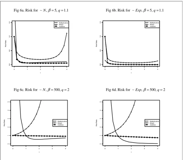
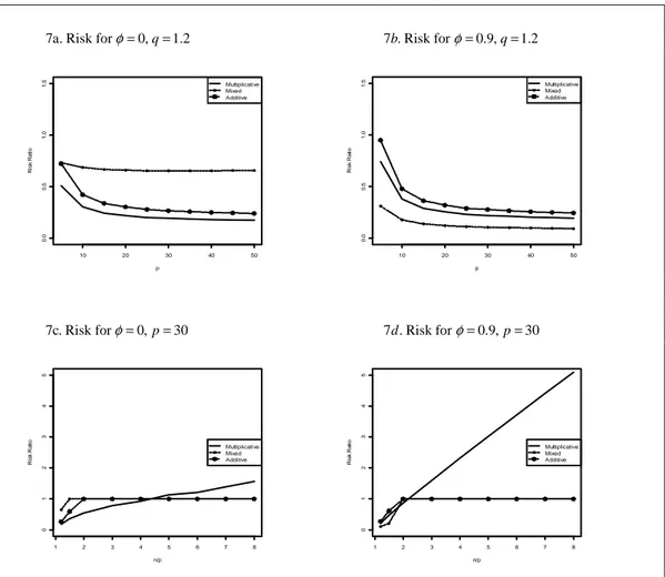
The estimators of the Mahalanobis distance are investigated in Figures 6 and 7. For low values of the scalar parameter β (Figure 6a and 6b) the ridge estimators perform very well while for values equal to 500 the standard estimator will dominate for a wide range of the ridge coefficient. Moreover, it is perhaps a bit surprising that the behavior of the estimators is drastically affected by the distribution; if the distribution is changed from a standard normal distribution to a standardized exponential distribution when q is low (Figure 6.a and 6.b) the relative performance of the ridge estimators improves markedly. This suggests that the standard estimator is more affected by asymmetric distributions than the ridge estimators. Moreover, from Figure 7 it is seen that all three adaptive estimators work very well, at least for values of q just above unity. But when q increases the multiplicative estimator asymptotically

0 50 100 150 200 0 .0 0 .5 1 .0 1 .5 p R is k R a ti o Multiplicative Mixed Additive 0 50 100 150 200 0 .0 0 .5 1 .0 1 .5 p R is k R a ti o Multiplicative Mixed Additive 2 4 6 8 10 0 .0 0 .5 1 .0 1 .5 n/p R is k R a ti o Multiplicative Mixed Additive 2 4 6 8 10 0 .0 0 .5 1 .0 1 .5 n/p R is k R a ti o Multiplicative Mixed Additive

22

deteriorates while the other two estimators limit the standard estimator. This, again, underlines the use of ridge estimators that coincide with the standard estimator for some value of the ridge coefficient.

{

}

{

}

2

Figure 6. R risk for Normal and Exponentiental distribution, = 5, 500 , β q= 1.1, 2 Fig 6a. Risk for ∼N,β=5,q=1.1 _{Fig 6b. Risk for} ∼_Exp,β=_5,q=_1.1

Fig 6c. Risk for ∼N,β=500,q=2 _{Fig 6d. Risk for} ∼_Exp,β=_500,q=₂

0 1 2 3 4 0 .0 0 .5 1 .0 1 .5 t R is k R a ti o Multiplicative Mixed Additive 0 1 2 3 4 0 .0 0 .5 1 .0 1 .5 t R is k R a ti o Multiplicative Mixed Additive 0 1 2 3 4 0 1 2 3 4 5 t R is k R a ti o Multiplicative Mixed Additive 0 1 2 3 4 0 1 2 3 4 5 t R is k R a ti o Multiplicative Mixed Additive

23

{

}

2

Fig 7. R risk for Normal distribution,β =5, φ∈ 0, 0.9

7a. Risk forφ=0,q=1.2 7 . Risk for b φ=0.9,q=1.2

7c. Risk forφ=0,p=30 7 . Risk for d φ=0.9,p=30

6 Conclusive Summary

This paper concerns the functional form of the estimator of the inverse covariance matrix. The main attention lies in settings where the dimension of the covariance matrix is comparable to the sample size, or even growing asymptotically. Specifically, three different ridge-type estimators have been investigated of which two are proposed by the authors and one has been considered previously in the literature. The estimators are characterized by their different functional form in that the ridge coefficient operates multiplicatively, additively or as a mixture of these two. Risk functions for choosing optimal values of the ridge coefficients are derived in the paper and their corresponding two-stage (adaptive) estimators are examined through Monte Carlo simulations, in which the properties of the three estimators are demonstrated to be very unlike. The mixture estimator has some tractable properties but is not optimal

10 20 30 40 50 0 .0 0 .5 1 .0 1 .5 p R is k R a ti o Multiplicative Mixed Additive 10 20 30 40 50 0 .0 0 .5 1 .0 1 .5 p R is k R a ti o Multiplicative Mixed Additive 1 2 3 4 5 6 7 8 0 1 2 3 4 5 n/p R is k R a ti o Multiplicative Mixed Additive 1 2 3 4 5 6 7 8 0 1 2 3 4 5 n/p R is k R a ti o Multiplicative Mixed Additive

24

for any of the parameter settings investigated in the paper. The additive ridge estimator on the other hand is shown to perform surprisingly well over a wide range of parameter settings which is interesting since it has not been considered previously in the literature. In particular, while the multiplicative estimator outperforms the additive only when the quotient between the sample size and the dimension is low, the additive estimator, as well as the mixture estimator, have the advantage of coinciding with the standard maximum likelihood estimator for a certain value of the ridge coefficient. The simulations reveal that the proposed adaptive estimators indeed coincides with the standard estimator precisely when it is optimal, i.e. when the sample size is large relative to the dimension. This is not achieved by the previously proposed multiplicative estimator due to its different functional form. Hence, even though the multiplicative estimator has superior properties for low values of the sample quotient the careful practitioner may for this reason prefer the additive estimator.

Moreover, three adaptive estimators of the Mahalanobis distance in high dimensional contexts are also proposed in the paper and appropriate risk functions have been derived for choosing the optimal ridge coefficient. Monte Carlo simulations show that the resulting estimators expectedly outperform the traditional estimator for a wide range of parameter settings. Hence a tool for outlier detection in high dimensional data is developed which should be useful in diagnostic analysis.

25 References

Anderson, T. W. (2003). An Introduction to Multivariate Statistical Analysis. Wiley. Bai, Z. D. and J.W. Silverstein, (1998). No eigenvalues outside the support of the limiting spectral distribution of large dimensional random matrices. The Annals of Probability. 26(1), 316-345.

Daniels, M. J. and Kass, R.E. (2001). Shrinkage estimators for covariance matrices. Biometrics, 57, 1173-1184.

Dey, D. K. and Srinivasan, C. (1985). Estimation of a Covariance Matrix Under Stein´s Loss. The Annals of Statistics, 13(4), 1581-1591.

Foster, J. An Application of the Wiener-Kolmogorov Smoothing Theory to Matrix Inversion. (1961) J. Soc. Indust. Appl. Math, 9, 387-392.

Girko. V.L. (1975). Random Matrices. Kiev. Vyshcha shkola. Dordrecht.

Girko. V.L. (1990). Theory of Random Determinants. Kluwer Academic Publishers. Dordrecht.

Girko. V.L. (1995). Statistical Analysis of Observations of Increasing Dimension. Kluwer Academic Publishers.

Goldstein, M. and Smith, A. F. (1974). Ridge-type Estimators for Regression Analysis. Journal of the Royal Statistical Society, B, 36, 284-291.

Gruber, M. H. (1998). Improving Efficiency by Shrinkage. Marcel Dekker.

Hoerl, A. E. and Kennard, R. W. (1970a). Ridge Regression: Biased Estimation for Nonorthogonal Problems. Technometrics, 12, 55-67.

Hoerl, A. E. and Kennard, R. W. (1970b). “Ridge Regression: Applications to Nonorthogonal Problems”. Technometrics, 12, 69-82.

Jonsson, D. (1982). Some Limit Theorems for the Eigenvalues of a Sample Covariance Matrix. J. Multivar. Analaysis. 12(1), 1-38.

Kibria, B. M. G. (2003). Performance of Some New Ridge Regression Estimates. Communications in Statistics-Simulation and Computation, 32(2), 419-435.

Kolmogorov, A. N. and Fomin, S.V. (1957). Elements of the Theory of Functional Analysis. Vol 1. Graylock Press. Rochester, N. Y.

Kubokawa, T. and Srivastava, M.S. (2003) . Estimating the Covariance Matrix: a new approach. Journal of Multivariate Analysis, 86, 28-47.

26

Mahalanobis, P. C. (1936). On the generalised distance in statistics. Proceedings of the National Institute of Sciences of India 2 (1), 49-55.

Marchenko, V. A. and Pastur, L. A. (1967). Distribution of eigenvalues in certain sets of random matrices. Math. Sbornik, 72 (114). 507-536.

Mardia, K. V. (1970). Measures of multivariate skewness and Kurtosis with applications. Biometrika, 57(3), 519-530.

Mardia, K. V. (1977). (Krishnaiah, ed.) Mahalanobis Distances and Angles, Multivariate Analysis IV, North-Holland.

Newey, W. K. and West, D. K. (1987), A Simple Positive Semi-Definite, Heteroscedasticity and Autocorrelation Consistent Covariance Matrix. Econometrica, 55(3), 703-708.

Obenchain, R. L. (1975). Ridge Analysis Following a Preliminary Test of the Shrunken Hypothesis. Technometrics, 17(4), 431-441.

Obenchain, R. L. (1978). Good and optimal ridge estimators. Annals of Statistics, 6, 1111-1121.

Pavlenko, T. and von Rosen, D. (2001). Effect of dimensionality on discrimination. Statistics, 35(3), 191-213.

Rao, C. R. (1973). Linear Statistical Inference and Its Applications. Wiley. New York.

Serdobolskii, V.I. (1985). The resolvent and the spectral functions of sample covariance matrices of increasing dimension. Russian Mathematical Surveys, 40, 232-233.

Serdobolskii. V. I. (2000). Multivariate Statistical Analysis: A High-Dimensional Approach. Springer-Verlag. Dordrecht.

Serdobolskii. V. I. (2008). Multiparametric Statistics. Elsevier. Amsterdam.

Shäfer, J. and Strimmer, K. (2005). A Shrinkage Approach to Large-Scale Covariance Matrix Estimation and Implications for Functional Genomics. Statistical Applications in Genetics and Molecular Biology, 4(1), 1-28.

Silverstein, J. W. and Bai Z. D. (1995). On the Empirical Distribution of Eigenvalues of a Class of Large Dimensional Random matrices. Journal of Multivariate Analysis. 54(2), 175-192.

Srivastava, V. K. and Giles, D.E.A. (1987). Seemingly unrelated regression equation models- Inference and prediction. Marcel Dekker. New York.

27

Stein, C. (1956). Inadmissibility of usual estimator for the mean of a multivariate normal distribution. Proceedings of the Third Berkeley Symposium on Mathematical and Statistical Probability, University of California, Berkeley, Volume 1, pp.197-206. White, H. and Domowitz, I. (1984). Nonlinear Regression with Dependent Observations. Econometrica, 52 (1), 143-161.

Wilks, S. S. (1963). Multivariate Statistical Outliers. Sankhya A, 25, 407-426.

Yin, Y. Q., Bai, Z. D. And Krishnaiah, P. R. (1988). On the Limit of the Largest Eigenvalue of the Large Dimensional Sample Covariance Matrix. Probability Theory and Related Fields. 78(4), 509-521.

Zellner, A. (1962). An Efficient Method of Estimating Seemingly Unrelated Regression Equations and Tests for Aggregation Bias. Journal of the American Statistical Association, 58, 348-368.