IMF effect on the polar cap contraction and expansion during a period of substorms

(1)

This is the published version of a paper published in Annales Geophysicae.

Citation for the original published paper (version of record):

Aikio, A., Pitkänen, T., Honkonen, I., Palmroth, M., Amm, O. (2013)

IMF effect on the polar cap contraction and expansion during a period of substorms.

Annales Geophysicae, 31: 1021-1034

http://dx.doi.org/10.5194/angeo-31-1021-2013

Access to the published version may require subscription.

N.B. When citing this work, cite the original published paper.

Permanent link to this version:

(2)

Ann. Geophys., 31, 1021–1034, 2013 www.ann-geophys.net/31/1021/2013/ doi:10.5194/angeo-31-1021-2013

EGU Journal Logos (RGB)

Advances in

Geosciences

Open Access

Natural Hazards

and Earth System

Sciences

Open Access

Annales

Geophysicae

Open Access

Nonlinear Processes

in Geophysics

Open Access

Atmospheric

Chemistry

and Physics

Open Access

Atmospheric

Chemistry

and Physics

Open Access Discussions

Atmospheric

Measurement

Techniques

Open Access

Atmospheric

Measurement

Techniques

Biogeosciences

Open Access Open Access

Biogeosciences

Discussions

Climate

of the Past

Climate

of the Past

Discussions

Earth System

Dynamics

Earth System

Dynamics

Discussions

Geoscientific

Instrumentation

Methods and

Data Systems

Open Access

_{Geoscientific}

Instrumentation

Methods and

Data Systems

Geoscientific

Model Development

Geoscientific

Model Development

Discussions

Hydrology and

Earth System

Sciences

Open Access

Hydrology and

Earth System

Sciences

Ocean Science

Discussions

Solid Earth

Discussions

The Cryosphere

Natural Hazards

and Earth System

Sciences

Open Access

Discussions

IMF effect on the polar cap contraction and expansion during a

period of substorms

A. T. Aikio1, T. Pitk¨anen1, I. Honkonen2,3, M. Palmroth2, and O. Amm2 1_{Department of Physics, University of Oulu, P.O. Box 3000, 90014, Finland} 2_{Finnish Meteorological Institute, P.O.Box 503, 00101, Helsinki, Finland} 3_{Department of Physics, University of Helsinki, P.O. Box 64, 00014, Finland}

Correspondence to: A. T. Aikio (anita.aikio@oulu.fi)

Received: 25 October 2012 – Revised: 26 April 2013 – Accepted: 9 May 2013 – Published: 12 June 2013

Abstract. The polar cap boundary (PCB) location and

mo-tion in the nightside ionosphere has been studied by us-ing measurements from the EISCAT radars and the MIRA-CLE magnetometers during a period of four substorms on 18 February 2004. The OMNI database has been used for obser-vations of the solar wind and the Geotail satellite for magne-tospheric measurements. In addition, the event was modelled by the GUMICS-4 MHD simulation. The simulation of the PCB location was in a rather good agreement with the exper-imental estimates at the EISCAT longitude. During the first three substorm expansion phases, neither the local observa-tions nor the global simulation showed any poleward moobserva-tions of the PCB, even though the electrojets intensified. Rapid poleward motions of the PCB took place only in the early recovery phases of the substorms. Hence, in these cases the nightside reconnection rate was locally higher in the recovery phase than in the expansion phase.

In addition, we suggest that the IMF Bz component

cor-related with the nightside tail inclination angle and the PCB location with about a 17-min delay from the bow shock. By taking the delay into account, the IMF northward turnings were associated with dipolarizations of the magnetotail and poleward motions of the PCB in the recovery phase. The mechanism behind this effect should be studied further.

Keywords. Magnetospheric physics (magnetospheric

con-figuration and dynamics; solar wind-magnetosphere interac-tions; storms and substorms)

1 Introduction

The polar cap boundary (PCB) is one of the most impor-tant boundaries in the ionosphere. It marks the ionospheric trace of the surface separating the closed field line region from the so-called open field lines close to the geomagnetic poles. Only space-borne optical imaging by satellites pro-vides the possibility to observe the PCB globally (Baker et al., 2000; Milan et al., 2003; Hubert et al., 2006). In addi-tion, several local methods exist, based on observations of the auroral emissions (Blanchard et al., 1995), in situ particle detection (Newell et al., 1996a,b), analysis of coherent radar backscatter (Chisham et al., 2004), or electron temperature from incoherent scatter radar (Østgaard et al., 2005; Aikio et al., 2006).

Magnetic reconnection on the dayside magnetopause and in the nightside magnetotail drive global plasma convection allowing energy, momentum and plasma to transfer from the solar wind into the magnetosphere and the ionosphere. The low-latitude dayside reconnection creates open flux whereas the nightside tail reconnection closes it. Thus, the amount of open flux in the magnetosphere is dependent on the balance between the average day- and nightside reconnection rates. As the open magnetic flux changes, also the size of the po-lar cap area changes (Siscoe and Huang, 1985; Cowley and Lockwood, 1992). In the substorm cycle, during the growth phase the dayside reconnection rate is usually higher than the nightside reconnection rate, so that the polar cap expands. During substorm expansion, reconnection at the near-Earth neutral line (NENL) becomes important and as open field lines start to reconnect in the magnetotail, the polar cap area

(3)

pi2

Fig. 1. AE index (top panel) and integrated currents over the MIRACLE chain in units of 105A (bottom panel). Pi2 pulsations from NUR in arbitrary units are added in the bottom panel. Grey areas denote expansion phases of substorms SS1–SS4.

starts to decrease. During the recovery phase, tail reconnec-tion still continues.

This study has two main goals. The first one is to compare the experimental estimates of the polar cap boundary location to a global MHD simulation and the second one is to study how the IMF affects the PCB motions during a time interval containing four substorms on 18 February 2004. The PCB is identified from the EISCAT incoherent scatter radar data by utilising the method described in Aikio et al. (2006) and applied in several studies together with satellite and MIR-ACLE magnetometer data (e.g. Aikio et al., 2008; Pitk¨anen et al., 2009a, b, 2011; Hubert et al., 2010). Global simula-tion is provided by GUMICS-4, which solves the ideal MHD equations in the solar wind and in the magnetosphere, and is coupled to the electrostatic ionosphere. The code struc-ture and setup are discussed in detail e.g. in Palmroth et al. (2006). The solar wind data is from the OMNI database and in this event, the data comes from the ACE satellite. The IMF data is used to calculate two coupling functions, the dayside reconnection voltage (Siscoe and Huang, 1985; Cowley and Lockwood, 1992; Milan et al., 2007, 2008) and the Newell coupling function (Newell et al., 2007). To gain more under-standing of the IMF effect on the magnetosphere–ionosphere system, we also use Geotail satellite data from the near-Earth magnetotail.

2 Data analysis

2.1 Substorms on 18 February 2004

The time interval studied is on 18 February 2004 from 15:00 to 24:00 UT (∼ 17:30–02:30 MLT in the Scandinavian sector). We identify the substorms based on the AE index (Fig. 1). The expansion phase starts when the AE index starts a rapid rise and it ends when the index has reached a max-imum (McPherron, 1995). In this case, the AE index is al-most entirely determined by the AL index: AU is small and slowly varying throughout the time interval studied (data not shown). Expansion phases are marked grey in Fig. 1 and each of them is followed by a recovery phase, not marked in the figure for clarity. During the recovery phases, the AE index generally decreases, but temporal increases also occur, so the exact start time of the recovery phase is somewhat uncer-tain. Pi2 magnetic pulsations recorded by the NUR station (56.8◦cgmLat) in the Scandinavian sector are shown in the bottom panel. Pi2 pulsations are generated at substorm on-sets, and at mid-latitudes they are expected to be seen within a few hours of MLT from the meridian of the substorm cur-rent wedge (see e.g. the short review in Kepko and Kivelson, 1999). The onsets of three last substorms are indeed associ-ated with a Pi2 burst, but not the first one at 16:00 UT.

The bottom panel of Fig. 1 shows the integrated total east-west equivalent current along a MIRACLE magnetome-ter chain in Scandinavia extending from 78.9◦N to 60.5◦N in geographic latitudes. The selected stations are located close to a constant cgm longitude (about 107◦) close to the

(4)

−10 0 10

Bz, By (nT)

2004−02-18, SW-based data delayed to bow shock

300 400 500 vel (km/s) 0 1 Pdyn (nPa) 15 16 17 18 19 20 21 22 23 24 0 20 40 60 Vday (kV) UT Bz By SS1 SS2 SS3 SS4

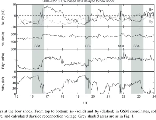
Fig. 2. IMF parameters at the bow shock. From top to bottom: Bz(solid) and By(dashed) in GSM coordinates, solar wind velocity, solar wind dynamic pressure, and calculated dayside reconnection voltage. Grey shaded areas are as in Fig. 1.

longitude of the EISCAT radar in Tromsø. The total current includes both the eastward and westward currents. These lo-cal currents are in good accordance with the AE index repre-senting a more global view.

Altogether four substorm expansion phases are seen (denoted by SS1–SS4), 16:00–16:48, 19:30–19:54, 21:42– 21:54, and 22:30–23:18 UT. The expansion phase of SS3 lasts only about 15 min and the increase in the AE index is hardly 300 nT, so it could be considered as a pseudo-breakup. As has been shown by several authors (e.g. Aikio et al., 1999), there is no substantial difference between the sub-storms and pseudobreakups, since both are associated with current wedge formation, particle injections at the geosyn-chronous orbit and magnetic reconnection in the near-Earth tail. However, pseudobreakups are smaller scale events than substorms with shorter duration and associated with only small or no poleward expansion.

Figure 2 top panel shows the IMF Bz and By

compo-nents in the GSM coordinates from the OMNI database (data delayed to the bow shock). As can be seen, all the sub-storms begin when the IMF is in the southward direction at the bow shock. During the period of interest By is

neg-ative (duskward). The solar wind velocity (second panel) stays at a very constant value, about 490 km s−1. The den-sity is small with values even below 1 cm−3before 16:36 UT and up to 3 cm−3after that (data not shown). The dynamic pressure (third panel) reflects mainly the changes in den-sity and it shows an increase at 16:36 UT to about 1.3 nPa. Another small steplike increase in pressure occurs at about 19:41 UT. Neither of these coincides with substorm onsets.

In conclusion, there is no indication of an external trigger of substorms.

2.2 Polar cap boundary and ionospheric currents

Measurements by the EISCAT VHF radar together with the EISCAT Svalbard radar (ESR) are used to identify the po-lar cap boundary (PCB) as described in Aikio et al. (2006). During 18 February 2004, the VHF radar was pointed at low elevation (30◦) to geographic north and the electron temper-ature measurements are used to calculate the PCB location between Tromsø (69.6◦N, 19.2◦E) and Svalbard (78.2◦N, 16.0◦E). The calculated geographic latitude of the PCB is shown by a black curve at 1-min data resolution in Fig. 3. There are two gaps in the curve, 17:30–19:00 and 19:25– 20:23 UT. The former is due to the fact that the PCB goes poleward of the ESR radar and the latter because the PCB comes too close to the VHF radar at Tromsø so that the radar beam does not cover the F region.

The colour surfaces in Fig. 3 are the equivalent currents calculated from the MIRACLE magnetometer network data along the central meridian by using the 1-D upward contin-uation method by Vanham¨aki et al. (2003) in geographic co-ordinates. The range is from 66◦_{to 79}◦_{ggLat, which}

corre-sponds to 63.4◦to 75.3◦cgmLat.

Red colours indicate eastward currents and yellow to blue colours indicate westward currents. As is well known, the electrojet current is eastward in the evening sector and west-ward in the morning sector. The polewest-ward boundaries of the electrojets are co-located with the poleward boundaries of the respective convection electric fields, which are in the

(5)

SS1 SS2 SS3 SS4

Fig. 3. Equivalent east-west currents calculated from the MIRACLE magnetometer data. Red colour indicates eastward and other colours westward flowing currents in units of mA m−1(scale on the right). The zero current corresponding to the MCRB is shown by a white curve and the PCB from EISCAT data by a black curve. Expansion phases of substorms SS1–SS4 are denoted by vertical solid lines in this figure.

northward and southward directions in the evening and morn-ing sectors, respectively. The poleward convection reversal boundary (CRB) is a proxy for the polar cap boundary (e.g. Nishitani et al., 2002) and e.g. the event study by Pitk¨anen et al. (2009a,b) shows that the PCB and the CRB follow closely to each other. The latitude where the equivalent east-west electrojets change direction according to magnetometer analysis, is called the latitude of the magnetic signature of the convection reversal boundary (MCRB), see e.g. Amm et al. (2005). However, since equivalent electrojets may deviate from the real electrojets, the MCRB may differ 0.5–1.5◦ in latitude from the CRB (e.g. Amm et al., 2000). Despite this drawback, the MCRB is a very useful proxy for the PCB, since the MIRACLE magnetometers cover a wide range of latitudes. The MCRB at 1-min resolution is shown by a white curve in Fig. 3. Indeed, the white and black curves overlap before 19:30 UT, and after that there is a tendency for the MCRB to be located about 1◦poleward of the EISCAT PCB, especially during Substorm 4. It has been shown in earlier studies (Amm et al., 2003; Pitk¨anen et al., 2009a,b) that this behaviour is typical in the morning sector and is probably caused by field-aligned currents.

Figure 3 shows that Scandinavia is in the eastward elec-trojet (EEJ) region until Substorm 2 onset at 19:30 UT, and within the westward electrojet (WEJ) region after Substorm 3 onset 21:42 UT. During Substorm 2 expansion and recovery, the Harang discontinuity region (the midnight sector shear flow region) is in the vicinity of Scandinavia.

The GUMICS-4 MHD simulation was used to calculate the polar cap boundary for this event. The simulation uses

solar wind parameters from the ACE satellite as input and the delay time to the dayside magnetopause of 46 min was estimated by Honkonen et al. (2011). Figure 4 top panel shows some selected views from the GUMICS simulation. The Northern Hemisphere is viewed from the +Z GSE di-rection, and the open field line region is shown by a violet colour. The colour coding represents the flux tube entropy according to Farr et al. (2008). The colours from blue to red correspond to entropy from small to large values and violet is zero entropy corresponding to lobe field lines. The PCB corresponds to the ionospheric trace of the first closed field lines adjacent to the lobe field lines. Continuous time series of GUMICS simulation results are shown by red lines in the middle and bottom panels. In the middle panel, the red curve represents the PCB latitude at the EISCAT longitude at 5 min resolution from the simulation. In addition, the PCB from the EISCAT measurement is shown by black squares and the MCRB by a blue curve.

The latitude of the PCB and its temporal evolution from the GUMICS simulation match surprisingly well the EISCAT and MIRACLE measurements, taking into account the many assumptions inherent in a global simulation. Be-tween 16:00 and 17:20 UT, the PCB from GUMICS is lo-cated about 1.5◦poleward of the EISCAT PCB and MCRB, but its temporal evolution is similar. All the boundaries start to contract poleward at about 16:45 UT, at the end of the ex-pansion phase of SS1. After the GUMICS PCB has reached the maximum latitude at 17:20 UT it starts immediately to go down in latitude. The MCRB and the EISCAT PCB show the equatorward motion later. For the EISCAT PCB, the start

(6)

72 73 74 75 76 77 78 79 80

81 EISCAT PCB (black), GUMICS PCB (red), MCRB (blue)

ggLat (deg) 16 17 18 19 20 21 22 23 24 4 6 8 10 12 x 10 12 UT PC area (m 2) SS1 SS2 SS3 SS4 1930 UT 1630 UT 1715 UT 2100 UT 2215 UT

Fig. 4. Top panel: Selected plots of the Northern Hemisphere from the GUMICS simulation with violet colour showing the polar cap (12:00 MLT is up and 06:00 MLT to the right, for further details see the text). Middle panel: PCB from EISCAT (black line and squares), PCB from the GUMICS simulation (red) and the MCRB (blue). Bottom panel: Polar cap area from the GUMICS simulation (red) and estimates of the polar cap area from EISCAT (black) and MIRACLE (blue). Grey shaded areas are as in Fig. 1.

time of the polar cap expansion cannot be determined, but for the MCRB it is between 18:00 and 18:25 UT. Around 19:00 UT all the three boundaries have the same latitude, but after that the EISCAT PCB and the MCRB go to lower lati-tudes than the GUMICS PCB.

During the expansion phase of SS2, there is no signifi-cant poleward expansion in any of the boundaries. During the recovery phase of SS2, the GUMICS PCB, the EISCAT PCB and the MCRB all show a similar poleward expansion. Again, right after having reached the maximum latitude at about 21:00 UT, the GUMICS PCB starts to move to lower latitudes. The EISCAT PCB and the MCRB start the equa-torward motion about 20 min later than the GUMICS PCB.

The short-lived expansion phase of SS3 is associated with no poleward expansion in any of the boundaries. Immedi-ately after the expansion phase of SS3, all the three bound-aries exhibit a small (about 1.5◦_{lat) and short-lived excursion}

to the north.

Substorm 4 seems to be different from the previous sub-storms, since it is associated with a poleward expansion of the EISCAT PCB and the MCRB within the expansion phase. The poleward contraction of the EISCAT PCB and the MCRB continue in the recovery phase and then also GUMICS simulates a poleward contraction.

The red curve in the bottom panel of Fig. 4 shows the po-lar cap area from the GUMICS simulation. Naturally, the PCB motion to the poleward direction is associated with a decrease in the polar cap area and vice versa. The variations in the polar cap area are large and in the beginning of ex-pansion phases areas are in the order of 1.2 × 1013m2, corre-sponding to the open magnetic flux of about 0.63 GWb. After Substorms 1 and 2, the open magnetic flux has decreased to a value half of that and the decreases take place in the recovery phases. During the open flux closure, the electrojets remain rather intense (Fig. 1, bottom panel). After the expansion phase of SS2, two intensifications in the electrojet are seen. These WEJ intensifications take place just equatorward of the PCB, and they bring the PCB poleward (Fig. 3, blue-coloured current intensifications). Substorm (pseudobreakup) 3 closes only about 15 % of the open flux, and that also takes place in the recovery phase. However, the local total current intensity (Fig. 1, bottom panel) has a maximum later, and again it is associated with a local intensification of the WEJ close to the PCB (Fig. 3, blue-coloured current intensification).

Normally, it is not possible to calculate the polar cap area from a local measurement like the EISCAT radar mea-surement. However, since the GUMICS PCB latitude at the EISCAT longitude is in a rather good agreement with the

(7)

EISCAT PCB latitude and the MCRB latitude, we have utilised the global GUMICS results in determining the lar cap area as follows. We have plotted the GUMICS po-lar cap area as a function of GUMICS PCB latitude, deter-mined at the longitude of the EISCAT measurement. The data points have been fitted to a second order polynomial. To get fits with small residuals, we had to subdivide the time interval into three parts, 16:35–19:35 UT, 19:35–21:35 UT and 21:35–24:00 UT. The reason is probably that the mag-netospheric configuration and the corresponding oval shapes changed between these times. The fitted functions have then been used to calculate the polar cap areas from the EISCAT PCB latitudes and from the MCRB latitudes and they are shown in the bottom panel of Fig. 4 as a black and blue curve, respectively.

The curves are now smoother than in the top panel, since a sliding average over 9 min and with a 5-min step is applied to the original 1-min EISCAT data. In this figure, the gaps in the EISCAT data are filled with linear interpolation. Since the magnetic data fluctuated more, we used 19-min averages with 5-min steps for the MCRB data. The blue (MCRB) and black (EISCAT) curves now reflect better the true tempo-ral variations in the polar cap area than the simulation (red curve). Since the EISCAT measurement did not capture the highest and lowest latitudes of the PCB, we use the varia-tions in the MCRB to estimate the changes in the open mag-netic flux content. During SS1–SS3, no open flux is closed during the expansion phases according to the experimental or simulation data. During the SS4 expansion, EISCAT and the MCRB show flux closure, but the GUMICS simulation does not. The main open flux closure takes place at the be-ginning of the recovery phases for the first three substorms, and the values from the MCRB are 0.32, 0.42 and 0.06 GWb, respectively. The small flux closure of SS3 supports the inter-pretation of a pseudobreakup. The last substorm closes about 0.19 GWb during the expansion phase. These figures are in accordance with Milan et al. (2007), who noted that on aver-age substorms close 0.3 GWb.

2.3 Dayside and nightside reconnection

To study how the IMF affects the amount of open flux in the magnetosphere and hence the polar cap area, we will use the approach by Siscoe and Huang (1985) and Cowley and Lockwood (1992), which can be formulated as follows by applying Faraday’s law

d8B

dt =Vday−Vnight, (1)

where 8Bis the open magnetic flux threading the polar cap, Vday is the reconnection rate (voltage) on the dayside,

pro-viding open flux, and Vnightis the reconnection rate (voltage)

on the nightside, closing open flux (both are positive quan-tities in the equation). Since the time-dependent dayside and nightside voltages are usually different, the polar cap area is

either decreasing or increasing and the polar cap boundary is moving.

To approximate the dayside reconnection voltage, we use the equation by Milan et al. (2008, 2007) which is given by

Vday=Leffvx q B2 y+Bz2sin2 θ 2 , (2)

where vxis the solar wind speed, Byand Bzthe IMF

compo-nents in GSM and θ the IMF clock angle. The expression is the Kan and Lee (1979) reconnection electric field multiplied by a characteristic scale length Leff=2.75 RE. The

charac-teristic scale length is obtained by fits to the data of Milan et al. (2007) and they show that in some cases Leffcan be a

factor of 1.6 larger.

The dayside reconnection voltage Vday is displayed in the

bottom panel of Fig. 2. In this case, when the solar wind ve-locity is almost constant and the Bycomponent stays

nega-tive, Vdayis almost a mirror image of Bz. Variations in Bzare

visible even during northward IMF in Vday, since Byis

non-zero and rather stable. Vdayis large during the growth phases

and close to zero at the end of the expansion phases or in the early recovery phases.

In principle, one could try to calculate the time deriva-tive of the open magnetic flux and then use Eq. (1) to de-rive Vnight. We have tested that, but there are two difficulties.

First, for time derivatives, strong smoothing of magnetic flux must be done, which results in poor time resolution. More serious is that obviously the numeric values of Vdaygiven by

Eq. (2) are sometimes too small (maximum values are about 60 kV), since negative values of Vnight were obtained at the

end of two growth phases.

Newell et al. (2007) studied different coupling functions and found that the function below correlated best with differ-ent magnetospheric state variables and geomagnetic indices

d8MP dt =v 4 3_B 2 3 Tsin 8 3 θ 2 , (3)

where BTis the magnitude of the transverse IMF at the

sub-solar magnetopause. Newell et al. argued that also this func-tion represents the rate magnetic flux is opened at the magne-topause and the difference to Eq. (2) is only somewhat differ-ent in expondiffer-ents. In addition, the Newell coupling function is not scaled to any physical units. The shapes of these two cou-pling functions given by Eqs. (2) and (3) are almost identical in this case as will be shown in Fig. 6. So, there is reason to believe that the time dependence of Vday is reasonably well

captured, but the actual magnitude of the voltage is uncertain.

2.4 Magnetospheric observations

For the studied time period, the GOES10 and 12 satellites were located on the dayside magnetosphere and hence their data could not be used to study the possible dipolarizations on the nightside. The LANL geosynchronous satellites show

(8)

Feb. 18, 2004 GEOTAIL MGF EFD LEP Editor-B GSM -15 -10 -5 0 5 10 Bx (nT) -10 -5 0 By (nT) -20 2 4 6 8 Bz (nT) 0.2 0.4 0.6 0.8 1.0 N (1/cc) 5.0∑103 1.0∑104 1.5∑104 2.0∑104 2.5∑104 Ti (eV) -1000-500 0 500 1000 1500 Vx (km/s) -1000 -500 0 500 Vy (km/s) -600 -400 -2000 200 400 600 Vz (km/s) TIME (UT) X-GSM (Re) Y-GSM (Re) Z-GSM (Re) 15:00 -22.2 -13.2 2.0 16:00 -22.2 -13.9 1.2 17:00 -22.2 -14.6 0.3 18:00 -22.2 -15.2 -0.6 19:00 -22.1 -15.8 -1.6 20:00 -22.0 -16.3 -2.5 21:00 -21.9 -16.8 -3.3 22:00 -21.7 -17.2 -4.0 23:00 -21.6 -17.7 -4.4 SS1 SS2 SS3 SS4

Fig. 5. Geotail data on 18 February 2004 from top to bottom: GSM magnetic field components Bx, By, Bz, number density, ion temperature, and GSM plasma velocity components Vx, Vy, Vzas a function of UT and satellite location. Grey shaded areas are as in Fig. 1.

particle injections associated with onsets of Substorms 2 and 3 (data not shown). During Substorm 1, there is a data gap.

The Geotail satellite was located in the dawnside magne-tosphere at a distance of about −22 REin the XGSMdirection

and it was moving away from the magnetic midnight. During 15:00–23:00 UT the MLT of Geotail changed slowly from about 03:00 to 05:00 MLT (YGSMfrom −13 to −17 RE) and

ZGSMfrom 2 to −5 RE.

Overview of Geotail data is shown in Fig. 5. During the period of interest, Geotail is mostly in the plasma sheet (PS) or plasma sheet boundary layer (PSBL), based on density and ion temperature (Ti). Most of the time Ti is 1–7 keV,

which is typical of PS/PSBL. Densities vary between about 0.05 and 0.3, mainly below 0.2 cm−3. These densities are rather low, since typical densities close to the PS flanks are 0.2–0.5 cm−3(Tsyganenko and Mukai, 2003; Nagata et al., 2008). However, several SW parameters affect the densities

in the geomagnetic tail: IMF polarity, solar wind speed and density. In this case, the SW density has been extremely low for an extended period, and is expected to affect the den-sities in the plasma sheet in a similar manner, as shown in Tsyganenko and Mukai (2003). During a few time intervals,

Ti drops to about 100 eV and densities go below 0.02 cm−3

(short periods between 16:00 and 17:00 UT, longer period around 20:00 UT), indicating that Geotail is moving into the lobe.

Before 15:45 UT Bx is nearly zero and Bzpositive.

Geo-tail is located in the Northern Hemisphere and the field is rather dipolar. After 15:45 UT Bxshows an abrupt

enhance-ment and Bz starts to decrease, indicating that field lines

start to stretch. This happens during the growth phase of the first substorm. At the same time, a large tailward (vx∼

−1000 km s−1) plasma flow starts at Geotail. This could in-dicate the beginning of near-Earth reconnection earthward of

(9)

0 0.2 0.4 0.6 0.8 1 −Vday −New07 Bz 2004−02−18 0 20 40 60 80

Geotail B incl angle

16 17 18 19 20 21 22 23 24 70 72 74 76 78 80 MCRB PCB gglat UT A A B C C D D E E F F E F SS1 SS2 SS3 SS4 B E

Fig. 6. IMF Bz(blue), negative of Vday (red), and negative of Newell et al. (2007) solar wind coupling function (black), all parameters normalised and delayed by 17 min from the bow shock (top), inclination angle in the magnetotail as measured by Geotail (middle), polar cap latitude in the nightside ionosphere as measured by EISCAT (blue squares, bottom) and convection reversal boundary as measured by the MIRACLE magnetometers (black solid line, bottom). Marked points (A–F) are used in the time delay analysis. Grey shaded areas are as in Fig. 1.

Geotail (XGSM> −22 RE) and it takes place 15 min before

the substorm onset as defined, based on the AE index (see Fig. 1).

At about 16:20 UT plasma flow turns earthward, reaches values up to 1400 km s−1and the fast flow lasts 10 min. It is followed by another earthward flow burst of 900 km s−1 be-tween 16:40 and 16:50 UT. These flows are associated with complex variations in magnetic field. Between the bursts, Bx

goes negative and after the second flow burst, Bx remains

negative, indicating that Geotail has moved from the North-ern Hemisphere to the SouthNorth-ern Hemisphere. These vari-ations take place during and in the end of the expansion phase of the first substorm: the recovery phase of the sub-storm starts at 16:48 UT according to the AE index. Possi-bly the earthward flows are associated with reconnection tak-ing place tailward of Geotail. Slavin et al. (2003) have stud-ied small flux ropes in the near-tail plasma sheet and found that all of them were embedded within either earthward or tailward directed high-speed plasma sheet flows. Analysing these magnetic structures in detail is out of scope of this pa-per.

Between 17:00 and 17:10, in the recovery phase of the first substorm, high values of plasma density are recorded (1 cm−3_{), indicating that the plasma sheet has expanded to}

engulf Geotail. At the same time, a small tailward flow is seen. After this short period, Geotail moves back to PSBL (n < 0.3 cm−3). Between 17:00 and 17:20, the absolute value

of Bxdecreases while Bzincreases, so the tail changes to a

more dipolar configuration. Fast plasma flows (magnitudes up to 400 km s−1) occur in the earthward direction (An-gelopoulos et al., 1994).

After 18:00 UT the tail starts slowly to stretch, indicating the beginning of a growth phase of Substorm 2. At 19:20 UT the magnitude of Bxincreases suddenly and the tail becomes

more stretched, plasma sheet thins and and Geotail moves from the PSBL to the tail lobe. Substorm 2 onset takes place 19:30 UT (Fig. 1) and the recovery phase starts at 19:54 UT, but only at 20:14 UT that Geotail observes the first signa-ture associated with it and then a tailward flow of about 200 km s−1 is observed, which is followed by an earthward flow (300 km s−1) starting from 20:16 UT. At 20:22 UT a new tailward flow burst of 500 km s−1starts and it changes to earthward flow of 600 km s−1 at 20:28 UT and lasts un-til 20:40 UT. In association with the flow bursts, Geotail has moved from the lobe to the PSBL, indicating thickening of the plasma sheet. After 20:46 UT the densities decrease, which indicate that Geotail is again in the lobe.

The expansion phase of Substorm 3 takes place 21:42– 21:54 UT and Geotail sees earthward plasma flow with a ve-locity below 500 km s−1_{21:50–22:00 UT. During Substorm}

4 Geotail has moved to the morning sector and close to the flank of the magnetosphere.

The magnetic field inclination angle in the magnetotail measured by Geotail is defined here by θ = arctan(−Bz/Bx)

(10)

and is shown in Fig. 6, middle panel. Here 0◦ _corresponds

to magnetic field in the −XGSMdirection (Geotail is in the

Southern Hemisphere for most of the time of interest). Dur-ing the expansion phase of SS1 before 16:48 UT, Geotail crosses the neutral sheet several times and is engulfed within flow bursts and complicated magnetic structures, so the in-clination angle varies rapidly and hence the angle is shown only after 16:30 UT.

The bottom panel of Fig. 6 shows the PCB latitude from EISCAT data (blue squares) and the MCRB latitude (black curve), both taken from Fig. 3. The Geotail inclination an-gle correlates well with the EISCAT PCB latitude so that a taillike configuration (small inclination angle) corresponds to a large polar cap (low PCB latitude), whereas a dipo-lar configuration (angle approaching 90◦) corresponds to a small polar cap (high PCB latitude). Even many details are reproduced like the short-lived increase in the EISCAT PCB latitude at 19:10 UT. However, there are also differ-ences. During 20:00–20:40 UT the inclination angle first in-creases and then dein-creases, whereas the EISCAT PCB lat-itude increases steadily from 20:21 UT onwards. However, the MCRB shows a similar bump. Still after 22:00 UT, in the SS3 recovery phase, the EISCAT PCB latitude, the MCRB, and the Geotail inclination angle all show small excursion to a poleward direction, but after that only little variation in Geotail data can be seen. At 23:00 UT Geotail is approaching 05:00 MLT and is getting closer and closer to the flank of the magnetosphere.

2.5 IMF effect on the tail configuration and on the PCB

The top panel of Fig. 6 shows the following parameters: the IMF Bz component, the negative of Vday, and the negative

of the Newell solar wind coupling function “New07” from Eq. (3), all normalised between 0 and 1. The sign information of the IMF Bzhas been lost in the normalisation, but can be

seen from Fig. 2, top panel. Small values of the normalised

Bz correspond to the southward IMF and large values (up

to 1) to the northward IMF. Small values of the normalised

−Vdayand −New07 correspond to large values of the solar

wind coupling functions. One can see that all the parameters in the top panel have a very similar time dependence, indicat-ing that the IMF Bzis the main factor affecting both of the

functions.

The IMF Bzand the negatives of the related coupling

func-tions show a clear resemblance with the Geotail inclination angle and the PCB latitude. To estimate the time delay be-tween the dayside (bow shock) functions in the top panel of Fig. 6 (already delayed in the figure) and the nightside func-tions in the middle and bottom panels, we search for clear turning points in the curves. The selected local minima in the IMF Bz curve are marked by letters from A to F in the top

panel of Fig. 6. From Geotail data (middle panel), A can not be determined since flux ropes or corresponding structures were observed at that time. During D, Geotail measured

al-ternating earthward and tailward fast flows which were ob-viously associated with some localised magnetic structures including a high frequency component, and during F Geotail had moved close to the flank of the morning magnetosphere. So, from the Geotail data we are able to identify local min-ima B, C and D. From the MCRB curve (bottom panel of Fig. 6) two points are not estimated: the currents were very weak during B (Fig. 3), so the MCRB can not be estimated very well, and during C there were several local intensifica-tions of the oval currents affecting the MCRB location. From the MCRB curve, we determine points A, D, E and F. The PCB from EISCAT (bottom panel of Fig. 6, blue squares) suffers from the limited latitudinal extent of the observations and hence only E and F can be determined. In summary, from the middle and bottom panels of Fig. 6, we obtain altogether nine time estimates for comparison with the IMF Bz data.

The calculated mean of the time delay is 17.0 min and the standard deviation is 2.7 min. This time delay has been ap-plied to the top panel of Fig. 6.

During the whole time period, the IMF northward turn-ings (Bz increasing) and associated decreases in the

day-side reconnection voltage and the Newell coupling function are closely correlated with dipolarizations of the magneto-tail and poleward motions of the nightside PCB. However, the IMF northward turnings are very abrupt, whereas the changes in the nightside tail configuration and the PCB lo-cation are more gradual. In specific, the dipolarizations and PCB poleward motions starting at about 16:50, 20:00, 22:00 and 23:20 UT are all associated with northward turnings of the IMF with the 17-min delay.

The IMF starts to turn in a southward direction approx-imately after 17:30 UT and this turning is gradual. Espe-cially between 18:00 and 20:00 UT the correlation between the IMF Bz(and the negatives of the coupling functions) with

the Geotail inclination angle and the PCB latitude is very clear. Hence, the dayside reconnection obviously affects di-rectly the tail configuration and the nightside polar cap lati-tude by adding new magnetic flux in the magnetotail. Later, after 22:00 UT the IMF change from the south to the north and back to the south is associated with a similar change in the PCB location and Geotail inclination angle. Further im-plications of these correlations are discussed in the next sec-tion.

3 Summary and discussion

As in the earlier papers cited in Sect. 1, the EISCAT PCB and the MCRB determined from the MIRACLE magnetome-ters were in very good accordance for most of the stud-ied time interval. After the local magnetic midnight (about 21:30 UT), the MCRB was located up to 2◦poleward of the EISCAT PCB, which is a feature typical of morning sector (see Sect. 2.2).

(11)

A new aspect in this study is the comparison to a global simulation. The GUMICS-4 MHD model results of the polar cap boundary location and motion showed a general agree-ment with the EISCAT PCB and the MCRB. The polar cap contractions started at about the same time, but the polar cap expansions in the GUMICS simulation started immediately after the polewardmost PCB latitude had been reached. The poleward expansion of Substorm 4 took place in GUMICS about 30 min later than observed. These results resemble the study presented in Palmroth et al. (2004), where the simu-lation substorm was a half an hour faster than the observed substorm and the onset was about a half an hour later than the observed one.

The other main aspect of this study was to gain an un-derstanding of the role of solar wind effects on the observed polar cap motions and substorm dynamics. In the standard picture of substorms, the nightside field lines start to stretch when the IMF turns southward in the beginning of the growth phase. A near-Earth neutral line (NENL) is formed in the late growth phase or in the beginning of the expansion phase. First, closed field lines are merged, but on a time scale of minutes open field lines start to reconnect. Because the re-connection rate is proportional to the Alfv´en speed of the inflowing plasma, the process is relatively slow as long as it remains on the closed magnetic field lines where plasma is abundant. After the last closed field line is reached, the recon-nection rate increases abruptly. During the recovery phase, the substorm X-line moves very rapidly down the magne-totail. Concurrently, the earthward part of the plasma sheet expands and fills with hot plasma. The mid-tail plasma sheet thickening is associated with fast earthward flows (e.g. Baker et al., 2005).

The solar wind effect on the dayside magnetopause is global, but substorm dynamics depend on the MLT of the observation point in the nightside magnetosphere. Below we summarise the main observations by EISCAT, MIRACLE and the Geotail satellite as well as the GUMICS simulation during the four substorms SS1–SS4.

During the expansion phase of SS1, Scandinavia was not located within the substorm current wedge, but measured en-hanced EEJ in the evening sector (18:30–19:18 MLT). The local PCB was slowly moving equatorward. Geotail in the mid-tail was located at 03:15 MLT at the onset time of SS1 and measured fast flows and complex magnetic structures. Geotail location of X ∼ −22 REwas very close to the

aver-age NENL position at X ∼ −25 RE(e.g. Nagai et al., 1998),

so obviously flux ropes were moving past the Geotail loca-tion. In the beginning of the recovery phase, the local PCB in the evening sector contracted rapidly in the poleward direc-tion. The GUMICS polar cap area stayed constant during the expansion phase and started to decrease in the beginning of the recovery phase.

During the growth phase of SS2, MIRACLE measured eastward currents in the Scandinavian sector at about 22:30 MLT, and the PCB expanded equatorward. In the

be-ginning of the expansion phase of SS2, current direction changed abruptly westward, but the PCB remained in the south, actually equatorward of the EISCAT f-o-v. During the recovery phase of SS2, the PCB came to the f-o-v of EISCAT from the south and contracted rapidly polewards. Geotail measured a stretched tail configuration during the growth phase and the tail remained stretched during the expansion phase. During the recovery phase when the plasma sheet ex-panded, fast flows were measured. Again, the GUMICS po-lar cap area stayed constant during the expansion phase and started to decrease in the recovery phase.

Substorm 3 could be classified as a pseudobreakup. The PCB was moving in the equatorward direction close to the magnetic midnight during the growth and the short-lived pansion phases. Westward currents intensified during the ex-pansion phase and Geotail measured a burst of fast flows in the morning sector. GUMICS simulated an increase in the polar cap area during the growth phase, and the area stayed at a constant level in the late growth and expansion phases. In the beginning of the recovery phase, the local WEJ decreased in magnitude and the PCB experienced a small jump in the poleward direction. GUMICS modelled a small decrease in the polar cap area.

Substorm 4 followed immediately after SS3. Now, the lo-cal PCB in the post-midnight sector started to move in the poleward direction already in the expansion phase and the WEJ intensified. Geotail had moved close to the flank of the morning magnetosphere. GUMICS modelled slowly increas-ing polar cap area and the area started to decrease only at the end of the expansion phase. A very significant reduction in the polar cap area was modelled in the recovery phase.

In summary, the common feature in SS1–SS3 is that their expansion phases were not to associated with poleward mo-tions of the local polar cap boundary in the Scandinavian sector. For SS1, a plausible explanation is that EISCAT and MIRACLE were located in the evening sector within the re-gion of the eastward electrojet. For SS2 and SS3, Scandi-navia was located in the pre-midnight sector and obviously within the substorm current wedge region. Nevertheless, the poleward motion of the PCB took place only in the recovery phase. The global GUMICS simulation showed no decrease in open flux during any of the substorm expansion phases, but only in the recovery phases. This is in accordance with our local observations by EISCAT and MIRACLE for SS1–SS3, but not for SS4.

The absence of poleward expansion of the PCB means that the dayside reconnection is greater than or equal to the night-side reconnection according to Eq. (1). Only when Vnightis

greater than Vday, poleward expansion takes place. Several

recent observations support our findings. Milan et al. (2008) report that during 15 min in the beginning of an expansion phase aurora was expanding poleward, but auroral emissions remained inside the previously closed field line region. Milan et al. (2007) studied the durations of nightside closure events and found values up to 2.5 h with a mean of 70 min. The

(12)

mean value is larger than the typical duration of an expansion phase, so this suggests that reconnection may take place at a significant amount in the recovery phases. Recently, Lock-wood et al. (2009) have found that the nightside reconnection voltages maximise in the recovery phase.

The MIRACLE magnetometers showed that during recov-ery phases of Substorms 2–4, the westward electrojets con-tinued to be intense within the main oval, well separated from the PCB. In the late recovery phase of Substorm 2, short-lived (about 12 min) intensifications of the WEJ took place just equatorward of the PCB. Those could possibly be re-lated to poleward boundary intensifications (PBIs), which are known to occur in recovery phases, but also during quiet time periods. They have been associated with bursty bulk flows (BBFs) in the magnetotail (Zesta et al., 2000; Nakamura et al., 2001). Observations show that individual BBFs are rather narrow 1–3 RE(Sergeev et al., 1996; Nakamura et al., 2004)

and it has been suggested that they result from bursty recon-nection, which is supported by observations (e.g. Pitk¨anen et al., 2009a, b). Interestingly, Geotail located 05 MLT sep-arated from MIRACLE, observed fast flows exactly during the same time interval. This could suggest that the nightside reconnection region extended over a very large portion of the tail.

One important question is the definition of the recovery phase. Originally, the recovery phase was defined as the pe-riod when auroras, after having reached their polewardmost position, start to fade and retreat back to lower latitudes (Akasofu, 1964; McPherron, 1970). Because of the lack of continuous global auroral observations, it has become cus-tomary to define the start of the recovery phase as the period when the AE index starts to decrease from its peak value, or the AL index starts to increase from its minimum value (e.g. Baker et al., 1994; Kamide et al., 1996; Gjerloev et al., 2004; Juusola et al., 2011). It is not obvious that the maximum of AE would correspond to the changes in the magnetotail dis-cussed in the beginning of this section, since AE is a measure of global electrojet activity. In addition, because of the lim-ited number of stations used to derive the AE index, it may underestimate or even miss localised events.

To evaluate the role of the IMF on the substorm dynam-ics, we calculated two coupling functions that are related to the rate magnetic flux is opened at the magnetopause: the dayside reconnection voltage Vday(Milan et al., 2007, 2008)

and the Newell coupling function (Newell et al., 2007). Dur-ing the studied time interval, both of these functions were mainly determined by the IMF Bz variations and the

func-tional forms of the negatives of the coupling functions were almost identical to the IMF Bz.

By selecting clear turning points from the IMF Bz, Geotail

inclination angle, the MCRB and the EISCAT PCB, we esti-mated the delay between the IMF Bzat the bow shock and the

nightside ionosphere-magnetosphere parameters. We arrived at a value of 17.0 min with a standard deviation of 2.7 min. Correlation between the dayside coupling functions and the

nightside parameters was especially clear during the recov-ery phase of SS1 and the growth and the expansion phases of SS2. Let us first discuss the possible mechanisms and after that a plausible time delay.

When the IMF turns southward, merging of magnetic field lines at the dayside magnetopause takes place and Vday

in-creases. If the nightside reconnection rate is not increased to balance the dayside merging, the nightside near-Earth mag-netic field lines start to stretch and the polar cap area expands. This leads to a substorm growth phase and one could indeed expect correlation between Vday, the PCB latitude and the

near-Earth magnetic topology. During the expansion and re-covery phases, reconnection at the NENL is expected to take place, and if the nightside reconnection rate is higher than the dayside reconnection rate in Eq. (1), the tail becomes more dipolar and the polar cap area decreases. Hence, no corre-lation to Vday would be expected during the expansion and

recovery phases. However, if in the initial situation Vdayand

Vnightwould be large and balanced, and then Vdaywould start

to decrease while Vnight would stay at a constant level, this

would lead to an apparent control of Vday over the open flux

decrease. Since this is only speculation, the issue should be studied further.

The time delay from the dayside magnetosphere to the nightside is not well known. Lockwood and Morley (2004) estimated that the near-Earth tail is compressed by the addi-tional open flux from the dayside with a delay of 14 min. In this case, by using the observed solar wind speed of 490 km s−1, we get a travel time of 8 min from the bow shock (XGSM∼17 RE) to the Geotail distance of XGSM= −21 RE.

If we take into account a reduction of speed in the magne-tosheath by a factor of 0.8 (Lockwood and Morley, 2004), the travel time increases to 10 min. It is somewhat unclear what kind of an additional delay to 10 min is needed for the magnetic pressure change to affect the inner parts of the tail at this XGSM. If the propagation occurs with the Alfv´en

ve-locity and travels from the magnetopause ZGSM= −22 RE

(Shue et al., 1997) to the Geotail location of ZGSM= −2 RE,

the delay is 4.4 min, by using values of 7 nT for the tail lobe magnetic field and 0.1 cm−3for proton density when calcu-lating the Alfv´en velocity. Then the total time delay estimate is 14 min, which is within the 1-σ confidence limits of the estimated time delay of 17 min.

The time delay between the bow shock and Geotail loca-tion has also been estimated from the GUMICS-4 simula-tion in three dimensions by using the method of Andreeova et al. (2011). The structure followed in the simulation is the sudden pressure increase observed around 16:30 UT at the bow shock (Fig. 2). The normal direction of the shock is esti-mated by using the minimum variance method, and the shock speed is calculated from mass flux conservation. The shock appears to have first propagated through the dayside magne-topause and travelled into the tail inside the magnetosphere. The time delay from the bow shock to the Geotail location

(13)

is between 10 and 15 min, which is in accordance with the simple estimate presented above.

This event is special in one sense: the substorms followed a period of low geomagnetic activity, which was 2.7 days long. During this period, the IMF was mostly northward, so-lar wind speed steadily decreasing from 600 to 450 km s−1, the solar wind dynamic pressure was very low, the AE index remained below 300 nT and the SYM-H index was approach-ing zero. So, if there is a so called ground-state of magneto-sphere, one could expect that it had been reached before the studied event.

4 Conclusions

We have used the EISCAT incoherent scatter radars and the MIRACLE magnetometer network measurements to study the polar cap boundary (PCB) and the latitude of the mag-netic signature of the convection reversal boundary (MCRB) during a series of four substorms on 18 February 2004. The results have been compared to a global GUMICS-4 MHD simulation. In addition, the Geotail satellite measurements in the tail and the IMF data delayed to the bow shock have been utilised. The main results are as follows.

The GUMICS-4 simulation of the PCB locations at the EISCAT longitude showed a rather good agreement with the experimental estimates. The MCRB, which is the lati-tude where the equivalent east-west electrojets change di-rection according to the MIRACLE magnetometer analy-sis, followed the temporal variations seen in the EISCAT PCB location. During the expansion phases of the first three substorms, the local observations or the global simulation showed no significant poleward motions of the PCB, even though the local electrojets intensified. During the expansion phases of Substorms 2 and 3, EISCAT and MIRACLE were obviously located within the substorm current wedge region. Nevertheless, rapid poleward motions of the PCB took place only in the early recovery phases of the substorms. Hence, we suggest that at least locally, the nightside reconnection rate may be higher in the recovery than in the expansion phase. This is in line with the studies by Milan et al. (2007), Milan et al. (2008) and Lockwood et al. (2009).

The inclination angle of the magnetic field at XGSM∼

−22 RE, measured by Geotail, showed good correlation with

the EISCAT PCB and the MCRB latitudes, even though the measurements were made in different MLT sectors. A large polar cap (low PCB latitude) corresponded to a stretched tail configuration in the near-Earth tail and a small polar cap to a more dipolar configuration, as could be expected.

To evaluate the role of the IMF on the substorm dynamics, we calculated two coupling functions that are related to the rate magnetic flux is opened at the magnetopause: the day-side reconnection voltage Vday(Milan et al., 2007, 2008) and

the Newell coupling function (Newell et al., 2007). During the time interval studied, both of these functions were mainly

determined by the IMF Bzvariations. By selecting clear

turn-ing points from the IMF Bz, the tail inclination angle, the

MCRB and the EISCAT PCB, we estimated the time delay between the IMF Bzand the nightside parameters. We arrived

at a value of 17.0 min with a standard deviation of 2.7 min. The propagation time from the bow shock to the Geotail lo-cation was estimated in two different ways, which yielded values within 10–15 min. Hence, the 17-min delay seems to be physically reasonable. The correlation during the growth phase can be explained rather easily, but the reason for the correlation during the expansion and recovery phases is not obvious and should be studied further.

Acknowledgements. We thank R. Kuula for the help in analysing

the data. Geotail magnetic field, electric field and plasma data were provided by T. Nagai, H. Hayakawa and Y. Saito through DARTS at Institute of Space and Astronautical Science, JAXA in Japan. EISCAT is an international association supported by China (CRIRP), Finland (SA), Japan (STEL and NIPR), Germany (DFG), Norway (NFR), Sweden (VR) and United Kingdom (STFC).

Topical Editor I. A. Daglis thanks S. W. H. Cowley and J. Gjer-loev for their help in evaluating this paper.

References

Aikio, A. T., Sergeev, V. A., Shukhtina, M. A., Vagina, L. I., Angelopoulos, V., and Reeves, G. D.: Characteristics of pseu-dobreakups and substorms observed in the ionosphere, at the geosynchronous orbit and in the mid-tail, J. Geophys. Res., 104, 12263–12287, 1999.

Aikio, A. T., Pitk¨anen, T., Kozlovsky, A., and Amm, O.: Method to locate the polar cap boundary in the nightside ionosphere and application to a substorm event, Ann. Geophys., 24, 1905–1917, doi:10.5194/angeo-24-1905-2006, 2006.

Aikio, A. T., Pitk¨anen, T., Fontaine, D., Dandouras, I., Amm, O., Kozlovsky, A., Vaivdas, A., and Fazakerley, A.: EISCAT and Cluster observations in the vicinity of the dynamical polar cap boundary, Ann. Geophys., 26, 87–105, doi:10.5194/angeo-26-87-2008, 2008.

Akasofu, S.-I.: The development of the auroral substorm, Planet. Space Sci., 12, 273–282, 1964.

Amm, O., Janhunen, P., Opgenoorth, H. J., Pulkkinen, T. I., and Viljanen, A.: Ionospheric shear flow situations observed by the MIRACLE network, and the concept of Harang Discontinuity, AGU monograph on magnetospheric current systems, Geophys-ical Monograph, 118, 227–236, 2000.

Amm, O., Aikio, A., Bosqued, J.-M., Dunlop, M., Fazakerley, A., Janhunen, P., Kauristie, K., Lester, M., Sillanpää, I., Tay-lor, M. G. G. T., Vontrat-Reberac, A., Mursula, K., and André, M.: Mesoscale structure of a morning sector ionospheric shear flow region determined by conjugate Cluster II and MIRA-CLE ground-based observations, Ann. Geophys., 21, 1737– 1751, doi:10.5194/angeo-21-1737-2003, 2003.

Amm, O., Donovan, E. F., Frey, H., Lester, M., Nakamura, R., Wild, J. A., Aikio, A., Dunlop, M., Kauristie, K., Marchaudon, A., Mc-Crea, I. W., Opgenoorth, H.-J., and Strømme, A.: Coordinated studies of the geospace environment using Cluster, satellite and

(14)

ground-based data: an interim review, Ann. Geophys., 23, 2129– 2170, doi:10.5194/angeo-23-2129-2005, 2005.

Andreeova, K., Pulkkinen, T. I., Juusola, L., Palmroth, M., and Santolik, O.: Propagation of a shock-related disturbance in the Earth’s magnetosphere, J. Geophys. Res., 116, A01213, doi:10.1029/2010JA015908, 2011.

Angelopoulos, V., Kennel, C. F., Coroniti, F. V., Pellat, R., Kivelson, M. G., Walker, R. J., Russell, C. T., Baumjohann, W., Feldman, W. C., and Gosling, J. T.: Statistical characteristics of bursty bulk flow events, J. Geophys. Res., 99, 21257–21280, 1994.

Baker, D. N., Pulkkinen, T. I., Hones Jr., E. W., Belian, R. D., McPherron, R. L., and Angelopoulos, V.: Signatures of the sub-storm recovery phase at high-altitude spacecraft J. Geophys. Res., 99, 0967–10979, 1994.

Baker, J. B., Clauer, C. R., Ridley, A. J., Papitashvili, V. O., Brit-tnacher, M. J., and Newell, P. T.: The nightside poleward bound-ary of the auroral oval as seen by DMSP and the ultraviolet im-ager, J. Geophys. Res., 105, 21267–21280, 2000.

Baker, D. N., McPherron, R. L., and Dunlop, M. W.: Cluster ob-servations of magnetospheric substorm behavior in the near- and mid-tail region, Adv. Space Res., 36, 1809–1817, 2005. Blanchard, G. T., Lyons, L. R., Samson, J. C., and Rich, F. J.:

Locat-ing the polar cap boundary from observations of 6300 ˚A auroral emission, J. Geophys. Res., 100, 7855–7862, 1995.

Chisham, G., Freeman, M. P., and Sotirelis, T.: A statistical comison of SuperDARN spectral width boundaries and DMSP par-ticle precipitation boundaries in the nightside ionosphere, Geo-phys. Res. Lett., 31, L02804, doi:10.1029/2003GL019074, 2004. Cowley, S. W. H. and Lockwood, M.: Excitation and decay of solar-wind driven flows in the magnetosphere-ionosphere sys-tem, Ann. Geophys., 10, 103–115, 1992.

Farr, N. L., Baker, D. N., and Wiltberger, M.: Complexities of a 3-D plasmoid flux rope as shown by an MHD simulation, J. Geophys. Res., 113, A12202, doi:10.1029/2008JA013328, 2008.

Gjerloev, J. W., Hoffman, R. A., Friel, M. M., Frank, L. A., and Sigwarth, J. B.: Substorm behavior of the auroral electrojet in-dices, Ann. Geophys., 22, 2135–2149, doi:10.5194/angeo-22-2135-2004, 2004.

Honkonen, I., Palmroth, M., Pulkkinen, T. I., Janhunen, P., and Aikio, A.: On large plasmoid formation in a global mag-netohydrodynamic simulation, Ann. Geophys., 29, 167–179, doi:10.5194/angeo-29-167-2011, 2011.

Hubert, B., Milan, S. E., Grocott, A., Blockx, C., Cowley, S. W. H., and G´erard, J.-C.: Dayside and nightside reconnec-tion rates inferred from IMAGE FUV and Super Dual Au-roral Radar Network data, J. Geophys. Res., 111, A03217, doi:10.1029/2005JA011140, 2006.

Hubert, B., Aikio, A. T., Amm, O., Pitk¨anen, T., Kauristie, K., Mi-lan, S. E., Cowley, S. W. H., and G´erard, J.-C.: Comparison of the open-closed field line boundary location inferred using IMAGE-FUV SI12 images and EISCAT radar observations, Ann. Geo-phys., 28, 883–892, doi:10.5194/angeo-28-883-2010, 2010. Juusola, L., Ostgaard, N., Tanskanen, E., Partamies, N.,

and Snekvik, K.: Earthward plasma sheet flows dur-ing substorm phases, J. Geophys. Res., 116, A10228, doi:10.1029/2011JA016852, 2011.

Kamide, Y., Sun, W., and Akasofu, S.-I.: The average ionospheric electrodynamics for the different substorm phases, J. Geophys. Res., 101, 99–109, 1996.

Kan, J. R. and Lee, L. C.: Energy coupling function and solar wind magnetosphere dynamo, Geophys. Res. Lett., 6, 577–580, doi:10.1029/GL006i007p00577, 1979.

Kepko, L. and Kivelson, M.: Generation of Pi2 pulsations by bursty bulk flows, J. Geophys. Res., 104, 25021–25034, 1999. Lockwood, M. and Morley, S. K.: A numerical model of

the ionospheric signatures of time-varying magneticreconnec-tion: I. ionospheric convection, Ann. Geophys., 22, 73–91, doi:10.5194/angeo-22-73-2004, 2004.

Lockwood, M., Hairston, M., Finch, I., and Rouillard, A.: Trans-polar voltage and Trans-polar cap flux during the substorm cycle and steady convection events, J. Geophys. Res., 114, A01210, doi:10.1029/2008JA013697, 2009.

McPherron, R. L.: Magnetospheric dynamics, in: Introduction to Space Physics, edited by: Kivelson, M. and Russel, C. T., Cam-bridge University Press, 400–458, 1995.

McPherron, R. L.: Growth phase of magnetospheric substorms, J. Geophys. Res., 75, 5592–5599, 1970.

Milan, S. E., Lester, M., Cowley, S. W. H., Oksavik, K., Brittnacher, M., Greenwald, R. A., Sofko, G., and Villain, J.-P.: Variations in the polar cap area during two substorm cycles, Ann. Geophys., 21, 1121–1140, doi:10.5194/angeo-21-1121-2003, 2003. Milan, S. E., Provan, G., and Hubert, B.: Magnetic flux

trans-port in the Dungey cycle: A survey of dayside and night-side reconnection rates, J. Geophys. Res., 112, A01209, doi:10.1029/2006JA011642, 2007.

Milan, S. E., Boakes, P. D., and Hubert, B.: Response of the expand-ing/contracting polar cap to weak and strong solar wind driving: Implications for substorm onset, J. Geophys. Res., 113, A09215, doi:10.1029/2008JA013340, 2008.

Nagai, T., Fujimoto, M., Saito, Y., Machida, S., Terasawa, T., Naka-mura, R., Yamamoto, T., Mukai, T., Nishida, A., and Kokubun, S.: Structure and Dynamics of magnetic reconnection for sub-storm onsets with GEOTAIL observations, J. Geophys. Res., 103, 4419–4440, 1998.

Nagata, D., Machida, S., Ohtani, S., Saito, Y., and Mukai, T.: So-lar wind control of plasma number density in the near-Earth plasma sheet: three-dimensional structure, Ann. Geophys., 26, 4031–4049, doi:10.5194/angeo-26-4031-2008, 2008.

Nakamura, R., Baumjohann, W., Sch¨odel, R., Brittnacher, M., Sergeev, V. A., Kubyshkina, M., Mukai, T., and Liou, K.: Earth-ward flow bursts, auroral streamers, and small expansions, J. Geophys. Res., 106, 10791–10802, 2001.

Nakamura, R., Baumjohann, W., Mouikis, C., Kistler, L. M., Runov, A., Volwerk, M., Asano, Y., Vörös, Z., Zhang, T. L., Klecker, B., Rème, H., and Balogh, A.: Spatial scale of high-speed flows in the plasma sheet observed by Cluster, Geophys. Res. Lett., 31, L09894, doi:10.1029/2004GL019558, 2004.

Newell, P. T., Feldstein, Y. I., Galperin, Y. I., and Meng, C.-I.: Morphology of nightside precipitation, J. Geophys. Res., 101, 10737–10748, 1996a.

Newell, P. T., Feldstein, Y. I., Galperin, Y. I., and Meng, C.-I.: Cor-rection to “Morphology of nightside precipitation” by Patrick T. Newell, Yasha I. Feldstein, Yuri I. Galperin,and Ching-I. Meng, J. Geophys. Res., 101, 17419–17421, 1996b.

Newell, P. T., Sotirelis, T., Liou, K., Meng, C.-I., and Rich, F. J.: A nearly universal solar wind-magnetosphere coupling function in-ferred from 10 magnetospheric state variables, J. Geophys. Res., 112, A01206, doi:10.1029/2006JA012015, 2007.

(15)

Nishitani, N., Ogawa,T., Sato, N., Yamagishi, H., Pinnock, M., Vil-lain, J.-P., Sofko, G., and Troshichev, O.: A study of the dusk convection cell’s response to an IMF southward turning, J. Geo-phys. Res., 107, 1036, doi:10.1029/2001JA900095, 2002. Østgaard, N., Moen, J., Mende, S. B., Frey, H. U., Immel, T. J.,

Gal-lop, P., Oksavik, K., and Fujimoto, M.: Estimates of magnetotail reconnection rate based on IMAGE FUV and EISCAT measure-ments, Ann. Geophys., 23, 123–134, doi:10.5194/angeo-23-123-2005, 2005.

Palmroth, M., Janhunen, P., Pulkkinen, T. I., and Koskinen, H. E. J.: Ionospheric energy input as a function of solar wind param-eters: global MHD simulation results, Ann. Geophys., 22, 549– 566, doi:10.5194/angeo-22-549-2004, 2004.

Palmroth, M., Janhunen, P., Germany, G., Lummerzheim, D., Liou, K., Baker, D. N., Barth, C., Weatherwax, A. T., and Watermann, J.: Precipitation and total power consumption in the ionosphere: Global MHD simulation results compared with Polar and SNOE observations, Ann. Geophys., 24, 861–872, doi:10.5194/angeo-24-861-2006, 2006.

Pitk¨anen, T., Aikio, A. T., Kozlovsky, A., and Amm, O.: Recon-nection electric field estimates and dynamics of high-latitude boundaries during a substorm, Ann. Geophys., 27, 2157–2171, doi:10.5194/angeo-27-2157-2009, 2009a.

Pitk¨anen, T., Aikio, A. T., Kozlovsky, A., and Amm, O.: Corrigen-dum to “Reconnection electric field estimates and dynamics of high-latitude boundaries during a substorm” published in Ann. Geophys., 27, 2157–2171, 2009, Ann. Geophys., 27, 3007-3007, doi:10.5194/angeo-27-3007-2009, 2009b.

Pitk¨anen, T., Aikio, A. T., Amm, O., Kauristie, K., Nilsson, H., and Kaila, K. U.: EISCAT-Cluster observations of quiet-time near-Earth magnetotail fast flows and their signatures in the ionosphere, Ann. Geophys., 29, 299–319, doi:10.5194/angeo-29-299-2011, 2011.

Sergeev, V. A., Angelopulous, V., Gosling, J. T., Cattell, C. A., and Russell, C. T.: Detection of localized, plasma-depleted flux tubes or bubbles in the midtail plasma sheet, J. Geophys. Res., 101, 10817–10826, 1996.

Shue, J.-H., Chao, J. K., Fu, H. C., Russell, C. T., Song, P., Khurana, K. K., and Singer, H. J.: A new functional form to study the solar wind control of the magnetopause size and shape, J. Geophys. Res., 102, 9497–9511, 1997.

Siscoe, G. L. and Huang, T. S.: Polar cap inflation and deflation, J. Geophys. Res., 90, 543–547, doi:10.1029/JA090iA01p00543, 1985.

Slavin, J. A., Lepping, R. P., Gjerloev, J., Fairfield, D. H., Hesse, M., Owen, C. J., Moldwin, M. B., Nagai, T., Ieda, A., and Mukai, T.: Geotail observations of magnetic flux ropes in the plasma sheet, J. Geophys. Res., 108, 1015, doi:10.1029/2002JA009557, 2003. Tsyganenko, N. A. and Mukai, T.: Tail plasma sheet models de-rived from Geotail particle data, J. Geophys. Res., 108, 1136, doi:10.1029/2002JA009707, 2003.

Vanham¨aki, H., Amm, O., and Viljanen, A.: 1-dimensional up-ward continuation of the ground magnetic field disturbance us-ing spherical elementary current systems, Earth Planets Space, 55, 613–625, 2003.

Zesta, E., Lyons, L. R., and Donovan, E.: The auroral signature of earthward flow burst observed in the magnetotail, Geophys. Res. Lett., 27, 3241–3244, 2000.