ANALYSIS AND SUPPRESSION OF PASSIVE NOISE IN SURFACE MICROSEISMIC DATA
by
A thesis submitted to the Faculty and the Board of Trustees of the Colorado School of Mines in partial fulfillment of the requirements for the degree of Doctor of Philosophy (Geophysics). Golden, Colorado Date Signed: Farnoush Forghani-Arani Approved: Dr. Michael Batzle Professor of Geophysics Thesis Advisor Golden, Colorado Date Dr. Terence K. Young Professor and Head, Department of Geophysics
ABSTRACT
Surface microseismic surveys are gaining popularity in monitoring hydraulic fracturing processes. The effectiveness of these surveys, however, is strongly dependent on the signal-to-noise ratio of the acquired data. Cultural and industrial noise generated during hydraulic fracturing operations usually dominate the data, thereby decreasing the effectiveness of using these data in identifying and locating microseismic events. Hence, noise suppression is a crit-ical step in surface microseismic monitoring. In this thesis, I focus on two important aspects in using surface-recorded microseismic seismic data: first, I take advantage of the unwanted surface noise to understand the characteristics of these noise and extract information about the propagation medium from the noise; second, I propose effective techniques to suppress the surface noise while preserving the waveforms that contain information about the source of microseisms.
Automated event identification on passive seismic data using only a few receivers is challenging especially when the record lengths span long durations of time. I introduce an automatic event identification algorithm that is designed specifically for detecting events in passive data acquired with a small number of receivers. I demonstrate that the conventional ST A/LT A (Short-term Average/Long-term Average) algorithm is not sufficiently effective in event detection in the common case of low signal-to-noise ratio. With a cross-correlation based method as an extension of the ST A/LT A algorithm, even low signal-to-noise events (that were not detectable with conventional ST A/LT A) were revealed.
Surface microseismic data contains surface-waves (generated primarily from hydraulic fracturing activities) and body-waves in the form of microseismic events. It is challenging to analyze the surface-waves on the recorded data directly because of the randomness of their source and their unknown source signatures. I use seismic interferometry to extract the surface-wave arrivals. Interferometry is a powerful tool to extract waves (including body-wave and surface-body-waves) that propagate from any receiver in the array (called a pseudo
source) to the other receivers across the array. Since most of the noise sources in surface microseismic data lie on the surface, seismic interferometry yields pseudo source gathers dominated by surface-wave energy. The dispersive characteristics of these surface-waves are important properties that can be used to extract information necessary for suppress-ing these waves. I demonstrate the application of interferometry to surface passive data recorded during the hydraulic fracturing operation of a tight gas reservoir and extract the dispersion properties of surface-waves corresponding to a pseudo-shot gather. Comparison of the dispersion characteristics of the surface waves from the pseudo-shot gather with that of an active shot-gather shows interesting similarities and differences. The dispersion char-acter (e.g. velocity change with frequency) of the fundamental mode was observed to have the same behavior for both the active and passive data. However, for the higher mode surface-waves, the dispersion properties are extracted at different frequency ranges.
Conventional noise suppression techniques in passive data are mostly stacking-based that rely on enforcing the amplitude of the signal by stacking the waveforms at the receivers and are unable to preserve the waveforms at the individual receivers necessary for estimat-ing the microseismic source location and source mechanism. Here, I introduce a technique based on the τ − p transform, that effectively identifies and separates microseismic events from surface-wave noise in the τ − p domain. This technique is superior to conventional stacking-based noise suppression techniques, because it preserves the waveforms at individ-ual receivers. Application of this methodology to microseismic events with isotropic and double-couple source mechanism, show substantial improvement in the signal-to-noise ratio. Imaging of the processed field data also show improved imaging of the hypocenter location of the microseismic source. In the case of double-couple source mechanism, I suggest two approaches for unifying the polarities at the receivers, a cross-correlation approach and a semblance-based prediction approach. The semblance-based approach is more effective at unifying the polarities, especially for low signal-to-noise ratio data.
TABLE OF CONTENTS
ABSTRACT . . . iii
LIST OF FIGURES . . . vii
LIST OF TABLES . . . xiii
ACKNOWLEDGMENTS . . . xiv
Chapter 1 INTRODUCTION . . . 1
Chapter 2 AN AUTOMATED CROSS-CORRELATION BASED EVENT DETEC-TION TECHNIQUE AND ITS APPLICADETEC-TION TO A SURFACE PASSIVE DATASET . . . 8
2.1 Abstract . . . 8
2.2 Introduction . . . 9
2.3 Algorithm . . . 10
2.3.1 Cumulative cross-correlation . . . 11
2.3.2 Cross-correlation before or after Short-term Average/Long-term Av-erage? . . . 14
2.4 Application to passive data recorded at a Geothermal site . . . 16
2.5 Conclusion . . . 22
Chapter 3 UNDERESTIMATION OF BODY WAVES AND FEASIBILITY OF SUR-FACE WAVE RECONSTRUCTION BY SEISMIC INTERFEROMETRY 24 3.1 Abstract . . . 24
3.2 Introduction . . . 24
3.3 Analysis . . . 28
3.3.1 Limited number of stationary source locations for body wave . . . . 28
3.3.2 Small reflection coefficients . . . 32
3.3.3 Absence of sources under the reflector . . . 32
3.3.4 body waves are weak . . . 34
3.4 Application . . . 37
3.5 Conclusions . . . 43
Chapter 4 DISPERSION ANALYSIS OF PASSIVE SURFACE-WAVE NOISE GEN-ERATED DURING HYDRAULIC-FRACTURING OPERATIONS . . . 45
4.1 Abstract . . . 45
4.3 Field data description . . . 47
4.4 Dispersion analysis . . . 48
4.5 Dispersion analysis of active data . . . 49
4.6 Dispersion analysis of passive data . . . 50
4.7 Inversion for shear-wave velocity . . . 54
4.8 Discussion . . . 56
4.9 Conclusions . . . 59
Chapter 5 NOISE SUPPRESSION IN SURFACE MICROSEISMIC DATA . . . 61
5.1 Abstract . . . 61
5.2 Introduction . . . 61
5.3 Theory . . . 62
5.4 Data description . . . 63
5.5 Microseismic event with isotropic source mechanism . . . 65
5.6 Microseismic event with double-couple source mechanism . . . 67
5.7 Discussion and Conclusion . . . 74
Chapter 6 AN EFFECTIVE NOISE SUPPRESSION TECHNIQUE FOR SURFACE MICROSEISMIC DATA . . . 77
6.1 Abstract . . . 77
6.2 Introduction . . . 78
6.3 Methodology and processing steps for noise suppression . . . 79
6.3.1 Moveout correction . . . 80
6.3.2 Accounting for polarity change . . . 82
6.3.3 Noise suppression . . . 83
6.4 Semi-synthetic microseismic data recorded by an Areal Receiver Array . . . 84
6.5 Real/field surface microseismic data recorded by a star-shaped array . . . 89
6.5.1 Imaging . . . 94
6.6 Discussion and Conclusions . . . 95
Chapter 7 CONCLUSIONS AND RECOMMENDATIONS . . . 99
7.1 Conclusions . . . 99
7.2 Recommendations . . . 102
REFERENCES . . . 104
APPENDIX A MATHEMATICS OF INVERSE 2-D τ − P TRANSFORM . . . 112
APPENDIX B P-WAVE RADIATION PATTERN FOR AN ARBITRARY FAULT-PLANE . . . 115
LIST OF FIGURES
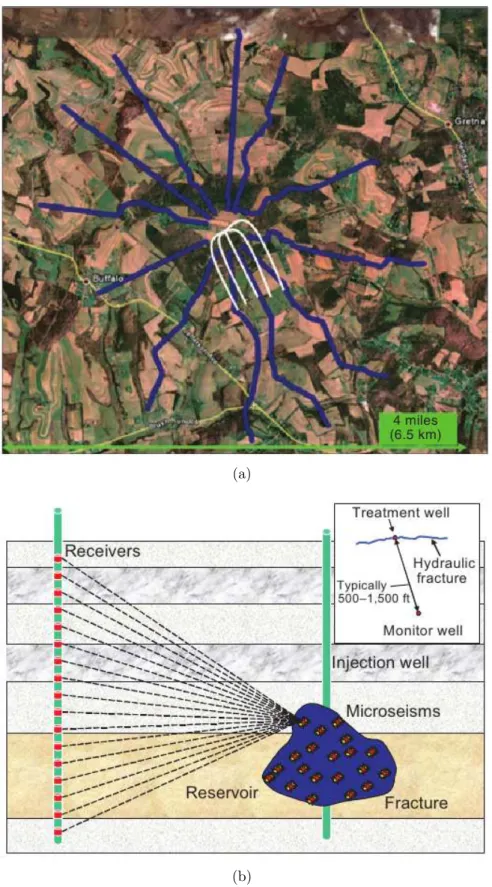
1.1 a) Plan-view of star-shaped surface microseismic array. The blue lines repre-sent the receiver array and the white lines in the center of the array denote horizontal treatment wells (Source: Duncan & Eisner (2010)). b) Schematic of borehole microseimsic acquisition (Source: Warpinski (2009)). . . 3 2.1 a) Seismogram of a synthetic microseismic event recorded at five receivers
at about 0.5 seconds; b) Computed ST A/LT A ratio of the seismogram in Figure 2.1(a); c) Summation of the local cross-correlation coefficients for the ST A/LT A ratios of Figure 2.1(b). . . 12 2.2 a) Seismogram-image of Figure 2.1(a); b) Computed ST A/LT A ratios of the
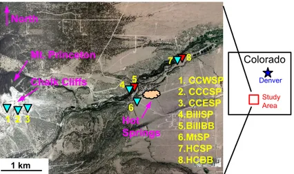
seismogram in Figure 2.2(a); c) Summation of the local cross-correlation co-efficients in Figure 2.2(b); d) Summation of the local cross-correlation coeffi-cients of the seismogram in Figure 2.2(a); e) Computed ST A/LT A ratios of the cross-correlation coefficients in Figure 2.2(d). . . 15 2.3 Location of passive seismic sensors at Mt. Princeton geothermal area; station
names SP (in blue triangle) and BB (in red triangle), denote the short-period and broad-band, respectively. . . 18 2.4 a) Seismogram of the Java earthquake recorded at our stations; traces in this
seismogram are normalized with respect to maximum amplitude at each trace. b) ST A/LT A ratio computed for the stations showing the earthquake event; c) Summation of the local correlation coefficients of the ST A/LT A ratios at the stations. . . 19 2.5 a) Seismogram of an event recorded at the eight stations at time 3:54 a.m.,
on September 23rd, 2009; traces in this seismogram are normalized with re-spect to maximum amplitude at each trace. b) Computed ST A/LT A ratio of the seismogram in Figure 2.5(a); c) Summation of the local cross-correlation coefficients for the ST A/LT A ratios of Figure 2.5(b). . . 21 3.1 a) Sources (stars) on a closed surface needed to reconstruct the full-wave
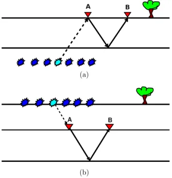
Green’s function between the two receivers (triangles) in a 2-D medium, b) sources needed to reconstruct the full-wave Green’s function when part of the closed surface is a free surface. Note that both a) and b) are side views of the distribution. . . 26
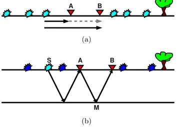
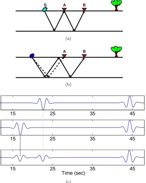
3.2 Illustration of two types of source-receiver distributions where, a) receivers are at the surface, sources are beneath the reflector; b) sources are at surface, receivers are in the interior. Note that sources in light blue have the largest contribution to the reconstruction of the reflected body wave between the two receivers. . . 26 3.3 A 2-Layer model in a 2-D medium . . . 28 3.4 Source locations that contribute to a) the surface wave reconstruction, b) the
body-wave reconstruction . . . 29 3.5 a) A stationary and b) a non-stationary source location for the reconstruction
of the body waves. c) The top and middle panels are the cross-correlations from the stationary and the non-stationary sources, respectively; the bot-tom panel is the average of the cross-correlations over stationary and non-stationary sources. The first arrival in the top panel is the body wave and the second arrival is the surface wave propagating between the two receivers. The first arrival in the middle panel is a non-physical arrival that is created by the non-stationary source. The second arrival is the surface wave. In the bottom panel, the first arrival is the non-physical arrival, the second and third arrivals are the body and surface waves, respectively, propagating between the two receivers. . . 31 3.6 Sources at the surface and underneath the reflector which give the dominant
contribution to the reconstruction of the reflected body wave between the two receivers. ρ and ρb are the densities of the upper and lower layers, respectively;
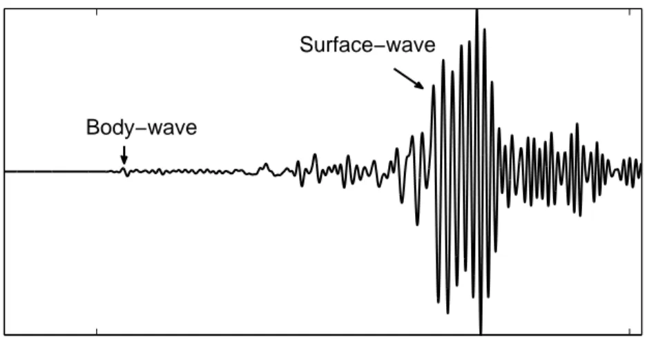
c is the velocity of the two layers. . . 33 3.7 Z-component seismogram for the 2004 Northern Sumatra earthquake
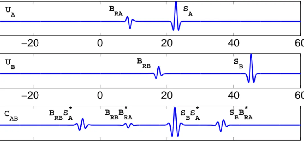
(magni-tude 9) recorded at KIEV (Kiev Ukraine), demonstrating the ampli(magni-tude ratio of the body to surface wave (Courtesy IRIS). . . 35 3.8 Loss of the body-wave amplitude by cross-correlation because of the low
am-plitude ratio of the body to the surface wave. Panels a) and b) show the waveforms at receivers A and B, respectively, recorded from source S shown in Figure 3.3. BRA, SA, BRB and SB are the body- and surface-wave terms
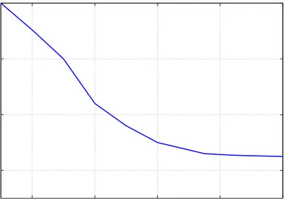
according to equations 3.3 and 3.4. Panel c) shows the cross-correlation of the waveforms in panels a) and b) according to equation 3.5. . . 37 3.9 Surface-wave velocity dispersion curve used in the synthetic model . . . 39 3.10 a) Plan view of the required sources (shown in light blue) for the reconstruction
of the direct surface waves in a 3-D medium; b) reconstruction of both direct and scattered surface waves (the solid line in the top panel) by summing over all the sources on the closed surface; reconstruction of the direct surface waves (solid line in the bottom panel) by summing over sources in light blue. The waveform shown in blue dashed line is the direct recorded Green’s function at one receiver from a source at the other receiver’s location. . . 40
3.11 a) Plan view of the required sources (shown in light blue) for the reconstruction of the scattered surface waves in a 3-D medium; b) reconstruction of both direct and scattered surface waves (the solid line in the top panel) by summing over all the sources on the closed surface; reconstruction of the scattered surface waves (solid line in the bottom panel) by summing over light blue sources. The waveform shown in blue dashed line is the direct recorded Green’s function at one receiver from a source at the other receiver’s location. . . 42 4.1 Map view of the receiver array used to acquire the active and passive data;
Black (outer array) and gray (central array) dots represent the receivers used for active records and gray dots indicate the receivers used for passive records. Black star represents the location of the active shot used in this study. . . . 47 4.2 (a) Active shot-gather recorded from the active source location shown by black
star in Figure 4.1; the traces are sorted by the distance to the shot, but trace number is not proportional to the distance. Note the fundamental and higher mode surface wave arrivals that are marked with black and white arrows, respectively. (b) τ − p image of the shot-gather in Figure 4.2(a). c) Disper-sion image of the active data obtained by applying 1-D Fourier transform to Figure 4.2(b). . . 51 4.3 Passive raw data . . . 52 4.4 (a) Pseudo shot-gather obtained by cross-correlation of receivers with the
pseudo-source shown by the black star in Figure 4.1. (b) τ − v image of the pseudo shot-gather in Figure 4.4(a). (c) Dispersion image of the active data obtained by applying 1-D Fourier transform to the τ − v image in Figure 4.4(b). 54 4.5 (a) Pseudo shot-gather obtained by cross-correlation of receivers with the
pseudo-source shown by the white star in Figure 4.1. (b) τ − v image of Figure 4.5(a). (c) Dispersion image of the active data obtained by applying 1-D Fourier transform to Figure 4.5(b). . . 55 4.6 a) Observed dispersion curves (shown in black) used to invert for shear-wave
velocity and predicted dispersion curves with high misfit (green) and low misfit (red) values; b) Acceptable shear-wave velocity models with high misfit (green) and low misfit (red) values. . . 57 4.7 Schematic of the receiver zone (blue shade) in which surface waves are
ex-tracted by interferometry from the passive noise sources in the red ellipse area; the pseudo-source (large black star) is located in (a) close to the noise sources and in (b) far from the noise sources. Black dots indicate the rest of receivers in the array for which surface waves can not be extracted. . . 58
5.1 Plan view of the receiver array at the Barnett shale reservoir; red and blue denote the central and outer part of the array, respectively. The two black lines denote the horizontal wells, and the black filled diamond represents the well head and the black empty diamonds represent the well bottom (Forghani et al., 2011). . . . 63 5.2 Plan view of the central receiver array. The black star is the surface location
of a synthetic microseismic event. . . 64 5.3 Surface passive data with an added isotropic microseismic event at about 2.7
seconds. Signal-to-noise (S/N) ratio is about 2. . . 66 5.4 Same data as in Figure 5.3 after sorting and moveout correction. Receivers
are sorted according to their distance from the epicenter of the microseismic source. . . 66 5.5 τ − p transform of the data in Figure 5.4. . . 67 5.6 Noise suppression result for the isotropic microseismic event in Figure 5.3.
The resulting signal-to-noise ratio is approximately 20. . . 68 5.7 Comparison of three waveforms: synthetic microseismic event (green), data
containing the microseismic event (blue), and result of noise suppression (red), for the isotropic source at one receiver location. . . 68 5.8 Simplified radiation pattern of a double-couple source; blue and red
repre-sent positive and negative polarities, respectively. Black arrows reprerepre-sent the coupled-forces. . . 69 5.9 Surface passive data with added double-couple microseismic event at about
2.7 seconds. Receivers are sorted according to the receiver lines and S/N is about 2. . . 70 5.10 Same data as in Figure 5.9 after sorting and moveout correction. Receivers
are sorted according to their distance from the epicenter of the microseismic source. . . 70 5.11 The data in Figure 5.10 after equalizing the polarity of the added
double-couple event using a cross-correlation-based technique. . . 71 5.12 τ − p transform of the data in Figure 5.11 (double-couple source). . . 72 5.13 double-couple microseismic event after applying noise suppression in τ − p
domain and inverse τ − p transform of Figure 5.12. Signal-to-noise ratio is about 15. . . 72 5.14 Comparison of three waveforms: synthetic microseismic event (green), data
containing the microseismic event (blue), and result of noise suppression (red), for the double-couple source at one receiver location. . . 73
5.15 a), d), and g): The surface passive data with added double-couple micro-seismic event at about 2.7 seconds with the signal-to-noise ratios of 1, 1.5, and 3, respectively. b), e), and h) are the passive data after applying noise suppression with the τ − p with the signal-to-noise ratios of 1.5, 10, and 25, respectively. c), f), and i): Comparison of three waveforms at one of the receivers in the array: synthetic microseismic event (green), combined micro-seismic event and passive data before noise suppression (blue), and combined microseismic event and passive data after noise suppression (red). . . 75 6.1 Flowchart of the processing steps for the noise suppression algorithm. . . 84 6.2 (a) Map view of the areal receiver array; gray dots represent the receivers. The
two black lines denote the horizontal wells, the black filled square shows the well head, and the black empty squares represent the well bottom (Forghani et al., 2012, 2011). (b) P-wave radiation pattern due to a double-couple source located in the center of the array at the reservoir depth; red and blue represent positive and negative polarities, respectively. . . 86 6.3 (a) Surface passive data with added microseismic event from a double-couple
source, recorded at about 2.75 seconds. Data are sorted according to the receiver in-lines. The signal-to-noise ratio which is estimated by dividing the root mean square (RMS) amplitude of the signal by that of the noise is about 2. (b) Same data as in Figure 6.3(a) after moveout correction. (c) The same data as in Figure 6.3(b) after unifying the polarity of the double-couple event using our semblance-based technique. (d) τ − p transform of the data in Figure 6.3(c). . . 87 6.4 (a) Microseismic event after applying noise suppression in τ − p domain and
inverse τ −p transform of Figure 6.3(d). Signal-to-noise ratio improves to ≈40. (b) Comparison of three waveforms: synthetic microseismic event (dotted gray), data containing the microseismic event (gray), and the result of noise suppression (black) for the double-couple source recorded at receiver number 115. . . 88 6.5 a), d), and g): Surface passive data with added microseismic event from a
double-couple source, recorded at about 2.75 seconds with the S/N of 1.5, 0.8 and 0.6, respectively. b), e), and h) are the passive data after applying noise suppression with the increase in S/N up to 30 and 4 , respectively, for the data in a) and d). c), f), and i): Comparison of three waveforms at receiver number 115: synthetic microseismic event (dotted gray), combined microseismic event and passive data before noise suppression (gray), and combined microseismic event and passive data after noise suppression (black). . . 90
6.6 (a) Star-shaped acquisition pattern containing 10 arms (receiver lines) used for surface microseismic monitoring over the Bakken Formation reservoir; black dots represent the receivers. (b) Predicted polarity at receivers using the semblance-based technique corresponding to a fracture-plane with strike, dip and slip angles of φ = 30◦
, θ = 70◦
, and ψ = 100◦
, respectively. . . 91 6.7 (a) A real microseismic event recorded at about 3.2 seconds. Receivers are
sorted according to the receiver arms. (b) Filtered data in Figure 6.7(a) with a band-pass filter of 10-55 Hz. (c) The same data as in Figure 6.7(b) after moveout correction and equalizing the polarity of the microseismic event using our semblance-based technique. (d) τ − p transform of the data in Figure 6.7(c). 93 6.8 (a) Data obtained by noise suppression applied to receivers in whole array.
(b) Result of sector-wise application of the noise suppression algorithm. . . . 94 6.9 Two-dimensional image of the hypocenter corresponding to the microseismic
event in (a) the data before noise suppression (Figure 6.7(b)) and (b) the data after noise suppression (Figure 6.8(a)). The velocity function Vz used for
imaging is given by Vz = 1800 + 0.5z m/s, where z is the depth. The velocity
model is laterally homogeneous and azimuthally isotropic. Data from a 30◦
azimuthal sector and its vertically-opposite sector (centered about the event epicenter) containing most of the receivers in arms 1, 10, and 6 (Figure 6.6(a)) are used for generating the above images. . . 96 B.1 Illustration of Euler angles; φ and θ are azimuth and dip of the fault-plane,
respectively. ψ denotes the slip angle and vectors ~ν and ~d represent the normal to the fault and the slip vector, respectively. . . 117
LIST OF TABLES
4.1 Survey parameters . . . 48 5.1 Data acquisition parameters of the surface passive seismic survey . . . 64 6.1 Data acquisition parameters of the surface passive seismic survey with an areal
receiver array. . . 85 6.2 Data acquisition parameters of the star-shaped acquisition in Figure 6.6(a). . 89
ACKNOWLEDGMENTS
My doctoral study could not be done without the support from my advisor, my co-advisor, committee members, staff, colleagues, friends, and family. First, I would like to thank my advisor Mike Batzle for his support and patience throughout the Ph.D. program. His expertise in practical problems have broaden my viewpoint in my research. In particu-lar, his friendly manner, good sense of humor and encouragement always made the though moments during my study much easier to handle. Also, his trust in me and what I was doing helped me to believe in myself and find my way out of the challenging moments. The deep insight and support from my co-advisor Roel Snieder in not only technical discussions but also real life problems was always an advantage for me. The best moments of chatting with Roel was when he always closed our meeting sessions with his ”really funny” jokes and discussed more broader aspects of life than just professional life. I am also thankful to Mark Willis and Seth Haines for their contribution not only as committee members but also as collaborators in the papers that shape my thesis and for their helpful insight and discussions throughout this thesis. The unlimited amount of time that they dedicated to discuss the research with me was very much beyond the expectations and showed their interest and con-cern for this research. Mark was always ready for long phone discussions from Houston, or long meetings during SEG conferences to make sure this research is moving. His encourage-ment was a great help during the challenging moencourage-ments of my graduate study. Many thanks to my committee members Paul Martin for his help to understand the mathematical aspects, Rich Krahenbul and Azra Tutuncu for their support and input for this thesis. Also, I would like to thank my former at large committee member Jennifer Miskimins for her support and encouragement during my study.
I am thankful to Terry young the head of Geophysics department and Nadine Young, for their support. The most supportive and kind staff at the Geophysics department like Barbara McLenan, Diane Witter, Michelle Szobody, Dawn Umpleby and Pamela Kraus whom in my
happy moments, I could share plenty of laughter with and in the tough moments I could receive lots of calming words from, gave me the best peace of mind.
I believe that every step froward toward finishing my thesis would not be possible with-out the support of the very helpful group of friends and colleagues around me. I am thankful to my colleagues at the Geophysics Department for their tremendous support during my study. The kindness and friendship of my friends and colleagues Steve Smith, Sonna Cot-taar, Gabriela Melo Silva, Mariana Carvalho, Patricia Rodriguez, Ivan Vasoncelos, Milana Aizenberg, Azar Hasanov and Yuanzhong Fan is unforgettable. Specially I am thankful to Steve Smith not only for his care and friendship, but also for his technical support and discussions in my research. The discussion and suggestions of the S-team members specially Kaoru Sawazaki, Michael Behm, Clement Flury, Conrad Newton and Nori Nakata were great help for me. I appreciate the help from my colleagues Bharath Shekar, Francesco Peronnie, Sjoerd de Ridder and Kris MacLennan in clarifying some of the technical questions. I am thankful for the companionship and support from Brian Passerella, Weiping Wang, Karoline Bohen and Jesse Havens during the long drives to the Mt. Princeton Geothermal field and their support for equipment maintenance.
The diversity of professional experts at the Geophysics Department is a valuable strength that provided an opportunity for me to broaden my knowledge. I am thankful to have the opportunity to communicate with and learn from Norm Bleistein, Steve Hill, Ken Larner, Dave Hale and Paul Sava. I also feel very lucky to have the opportunity of learning a lot from John Stockwell who I consider the ”treasure” of the Geophysics Department. His tremendous mathematical knowledge as well as his broad understanding of both theoretical and practical problems in Geophysics and more importantly his laid back personality and patience always invited me to ask him questions and bring up discussions.
The help and support for my thesis goes beyond the professional society. When I started at Mines, I was very new to Golden and my life was full of new things and uncertainties. I am happy to get to know Terry and Trudy Thompson who were great support and helped me to meet new people and make new friends with cultural variety. I am also very grateful to Norm Bleistein and Judy Armstrong for their kindness and care and for sharing all their
happy moments with us.
My appreciation to my family is beyond the words. Shayan with his love and smile, his care and kindness, and his enthusiasm about life and soccer has been always a great treasure in my life. At overwhelming times in my research, just one of his entertaining jokes or actions with the wide smile on his face would completely change my mood. Jyoti, a caring and supportive friend, a loving husband, and a great source of knowledge has always been a role model to me for his encouragement, hardworking and thoughtfulness as a person and a scientist. His great sense of humor at some moments and seriousness when it came to discuss research was very unique and joyful. I am so thankful to Shayan and Jyoti for the hard times that they had to go through because of me and I would not be able to finish this thesis without them.
I can not enough appreciate the care and support and unconditional love from my mom Tolo. During this journey, her support and kindness has always been a great fortune for me and my family. I am thankful for the support, love and help from my siblings Mozhdeh, Mehrdad and Ershad during my study. They have been always there whenever I needed them. I am also very grateful to my father- and mother-in-law Bapa and Maa and my brother and sister in-laws that have given me lots of support, love and encouragement to finish this thesis.
Dedicated to my son Shayan, my husband Jyoti and my mom Tolo for their infinite love and support
Chapter 1
INTRODUCTION
Low-permeability reservoir rocks such as shales and tight-gas sandstones are commonly stimulated using hydraulic fracturing to increase their permeability and enhance production. In order to maximize productivity, it is critical to distinguish zones that have been affected by hydraulic fracturing from zones that have not. A novel way of identifying these zones is to monitor the seismicity resulting from fracturing and stress changes (Cerda & Alfaro, 2007; Chambers et al., 2010; Eisner et al., 2010; Maxwell & Urbancic, 2001). The magnitude of these hydraulic-fracturing-induced seismic events is mostly less than 1, and they are usually referred to as microseismic events. Imaging of such microseismicity provides valuable information about fracture extent, fracture mechanism, and complexity which ultimately helps in estimating the stimulated reservoir volume and field-development planning. While hydraulic-fracture mapping is the most common application, microseismic monitoring is also conducted for geothermal systems (Romero et al., 1994; Feng & Lees, 1998; Majer et al., 2007), thermal-recovery processes, and reservoir surveillance (Warpinski, 2009).
Numerous considerations go into microseismic monitoring many of which are summa-rized in Warpinski (2009). They can be broadly categosumma-rized into acquisition, processing and interpretation of microseismic data. Important elements of acquisition include positioning of receivers, array design, and choice of sensors. Receivers may be placed close to the treatment wells in boreholes or they may be located on the surface. The above choice is determined by signal strength at the receivers, level of noise, aperture requirements, and economics. The number and location of receivers in an acquisition is also important because noise suppression can be more effective with increasing receivers and thus lead to better imaging of the data. The receivers should also be sensitive to the frequency content of the microseismic energy. According to Warpinski (2009), “The best sensors will be those with high sensitivity and a
flat response over the frequency range of interest.” In post-acquisition, the microseismic data is processed to suppress noise and locate arrivals corresponding to microseisms. Processing also involves recognition of P- and S-wave arrivals, polarization analysis and imaging. In the presence of strong noise, however, processing becomes extremely challenging. To locate microseismic hypocenters, the processed data is imaged using a velocity model. In most cases, the velocity model is obtained from nearby sonic logs or from inversion of surface reflection-seismic data. The quality of the image depends on the signal-to-noise ratio of the data and the accuracy of the velocity model.
Note that the common theme in all the above steps is the effect of noise. Noisy data resulting from poor acquisition or planning can lead to erroneous fracture mapping and will fail to meet the project objectives. Therefore, noise has to be treated at the acquisition stage or at the processing stage before interpretation. In this thesis, I address the noise issue at the processing stage.
Noise presents particularly in surface microseismic data. As mentioned above, monitor-ing of microseismicity can be done usmonitor-ing borehole or surface sensors (Figure 1.1). Although downhole monitoring places sensors close to the treatment well, it provides a limited record-ing aperture that may impose inaccuracy in microseismic hypocenter imagrecord-ing and source mechanism estimation (Thornton & Eisner, 2011; Eisner et al., 2010). Surface monitoring in the form of passive data is becoming more common in analyzing the hydraulic fracturing process (Kochnev et al., 2007; Duncan & Eisner, 2010). By passive data, I refer to the contin-uous recording of ground motion due to uncontrolled sources such as cultural and industrial activities. Because of the potentially larger receiver aperture and higher number of receivers, surface microseismic data may be more informative than downhole data (Eisner et al., 2010; Chambers et al., 2010; Duncan & Eisner, 2010). Yet the effectiveness of this technique is strongly dependent on the signal-to-noise ratio. Cultural and ambient noise usually dom-inate the data, thereby decreasing the effectiveness of surface microseismic techniques in identifying and locating microseismic events. Hence, noise suppression is a critical step in surface microseismic monitoring (Kochnev et al., 2007; Duncan & Eisner, 2010; Forghani et al., 2012, 2013).
(a)
(b)
Figure 1.1: a) Plan-view of star-shaped surface microseismic array. The blue lines represent the receiver array and the white lines in the center of the array denote horizontal treatment wells (Source: Duncan & Eisner (2010)). b) Schematic of borehole microseimsic acquisition
In this thesis, I address the issue of surface noise with two approaches. In the first ap-proach, I exploit the surface-wave noise to extract information necessary for its suppression; in addition, I explore ways in which the noise can also be used for extracting subsurface prop-erties. Under the second approach, I develop techniques that suppress noise while preserving the waveforms of the microseismic events.
The large amount of the surface passive records as well as the low signal-to-noise ratio of these data makes the use of these data challenging. Detection of events becomes especially difficult when only a few receivers are used in the survey. An automated, accurate algo-rithm is beneficial for event identification when processing days and months of passive data. Moreover, identifying an event in the case of low signal-to-noise ratio, specifically when the acquisition is limited to a few receivers, is challenging. ST A/LT A method is a commonly used automatic event identification algorithm which computes the ratio of the short term av-erage (STA) to the long-term avav-erage (LTA) of the passive seismic data. This technique has been primarily used to detect earthquakes in global seismology (Ambuter & Solomon, 1974; Chael, 1997; Withers et al., 1998) and later to detect microseismic events in unconventional oil/gas fields (Oye & Roth, 2003; Tan, 2007; Miyazawa et al., 2008a). I show in Chapter 2 that for the case of low signal-to-noise ratio and limited number of receivers, the ST A/LT A algorithm is not effective at event identification. Thereafter, I introduce a cross-correlation based technique as an extension of the ST A/LT A algorithm. The suggested technique takes advantage of the similarities of the ST A/LT A waveforms between receivers and improves the event detectability compared to the ST A/LT A algorithm. By providing examples of ap-plying the cross-correlation technique to synthetic data and a field surface passive dataset, I demonstrate the advantage of using this method over the conventional ST A/LT A algorithm. Instead of focusing only on noise suppression, an interesting strategy would be to exploit the noise to infer subsurface properties; also, understanding noise properties might help in their suppression. Therefore, I explore how seismic interferometry can help in extracting surface-noise properties. Although it is commonly thought that both body wave and surface waves can be extracted from interferometry, studies show underestimation of the body waves and dominance of surface waves when applying interferometry to the surface source-receiver
acquisition (Campillo & Paul, 2003; Shapiro & Campillo, 2004; Sabra et al., 2005b; Shapiro et al., 2005; Dong et al., 2006). This issue has created confusion in the applications of the interferometry and has not been clarified in the literature. In Chapter 3 I address this issue and investigate why in surface seismic interferometry mostly surface waves are extracted, while the body waves are not recorded well. The underestimation of the body waves by interferometry can in fact be beneficial for reconstruction/prediction of the surface waves that are mostly considered as unwanted noise in surface seismic data. In order to exploit the extracted surface waves from interferometry, it is important to understand to what extent these waves can be reconstructed. Therefore, I study the feasibility of the reconstruction of surface waves (direct as well as scattered surface waves) by interferometry. This analysis not only clarifies the underestimation of the body waves and limitations to the recovery of surface waves in a unique way, it also provides valuable insight into the understanding of interferometry applications to the surface passive data (as done in Chapter 4).
Apart from the event identification which was the focus of Chapter 2, another challenge of dealing with surface passive records is the presence of surface noise which can mask most of the subsurface arrivals, specifically the weak microseismic events that have traveled from a depth of a few kilometers to the surface. Understanding the surface-wave characteristics can be helpful for suppressing these noise. For example, dispersion characteristics of surface waves reveal the dominant wavelength of these waves which can be used for designing receiver arrays that can suppress part of these waves at the field (Baeten et al., 2000; Draganov et al., 2009). The focus of Chapter 4 is on extracting the surface-wave dispersive characteristics from a passive dataset. In Chapter 3 I show that application of interferometry to surface source-receiver acquisition yields data dominated by surface waves. In Chapter 4, I take advantage of this fact and apply the interferometry to data from surface receivers and sources (industrial noise) to extract the surface waves. Dispersion analysis is then applied to the extracted surface waves from interferometry. I also discuss the application of surface-wave dispersion in understanding the near-surface velocity and surface-wave noise suppression.
The processing and analysis in Chapters 3 and 4, yield sufficient understanding of the surface-wave characteristics and possible ways of suppressing these waves. Conventional
noise suppression techniques in passive data are mostly stacking-based that rely on enforcing the amplitude of the signal by stacking the waveforms at the receivers (Kiselevitch et al., 1991; Kao & Shan, 2004; Kochnev et al., 2007; Duncan & Eisner, 2010). However, waveforms at the individual receivers, which are necessary for estimating microseismic source location and source mechanism (Aki & Richards, 2002) cannot be extracted after processing with such methods.
In Chapters 5 and 6 I propose a noise suppression technique for the surface micro-seismic data based on transforming the data to the τ − p domain. While in the time-offset (t − x) domain, the characteristics of microseismic events might not be different from that of surface noise, in the τ − p domain, they show distinct characters which would help to separate them. With this suggested technique I aim to overcome the challenges in conven-tional techniques not only in terms of improving the signal-to-noise ratio of the microseismic events, but also preserving the waveforms at the individual receivers. The focus of both chapters is on the noise suppression. While in Chapter 5 I focus on demonstrating the processing and pre-processing steps for the suppression of the noise using simple models, in Chapter 6 I modify the modeling to be more realistic and apply some improvements in the processing steps. For example, the source mechanism considered in Chapters 5 is very sim-ple and does not include the realistic mechanism for which the radiation pattern is defined based on the orientations of a fracture-plane. In Chapters 6, I generate a more realistic microseismic source with the radiation pattern in which the polarities and the amplitude of the recorded waveforms vary with the fracture-plane orientation. In order to unify the polarities for an effective summation of waveforms in the τ − p transform, in Chapter 5 I apply cross-correlation to identify the polarities of the receivers. However, cross-correlation is not effective when the signal-to-noise ratio is low which is a common case in the surface microseismic data. Therefore, in Chapters 6 I suggest another technique for identifying the polarities, which is based on the semblance analysis. Another additional step different from Chapters 5 is that in Chapters 6 I apply my suggested noise suppression technique to field microseismic data to test its effectiveness on field data.
Chapter 2
AN AUTOMATED CROSS-CORRELATION BASED EVENT DETECTION TECHNIQUE AND ITS APPLICATION TO A SURFACE PASSIVE
DATASET
2.1 Abstract
In studies such as heavy oil, shale reservoirs, tight gas, and enhanced geothermal sys-tems, the use of surface passive seismic data to monitor induced microseismicity due to the fluid flow in the subsurface is becoming more common. However, in most studies passive seismic records contain days and months of data and manually analyzing the data can be expensive and inaccurate. Moreover, in the presence of noise, detecting the arrival of weak microseismic events becomes challenging. Hence, the use of an automated, accurate, and computationally fast technique for event detection in passive seismic data is essential.
The conventional automatic event identification algorithm computes a running-window energy ratio of the short-term average to the long-term average of the passive seismic data for each trace. We show that for the common case of low signal-to-noise ratio in surface passive records, the conventional method is not sufficiently effective at event identification. Here, we extend the conventional algorithm by introducing a technique that is based on the cross-correlation of the energy ratios computed by the conventional method. With our technique we can measure the similarities amongst the computed energy ratios at different traces. Our approach is successful at improving the detectability of events with low signal-to-noise ratio that are not detectable with the conventional algorithm. Also, our algorithm has the advantage to identify if an event is common to all stations (a regional event) or to a limited number of stations (a local event). We provide examples of applying our technique to synthetic data and a field surface passive dataset recorded at a geothermal site.
2.2 Introduction
Surface-recorded passive seismic data are being increasingly used for monitoring induced microseismicity resulting from fluid movement and/or stress changes in the subsurface. Re-cently, such data have become popular for remotely monitoring the hydraulic fracturing processes in oil and gas recovery (Cerda & Alfaro, 2007; Chambers et al., 2010; Duncan & Eisner, 2010; Eisner et al., 2010; Maxwell & Urbancic, 2001), and enhanced geothermal fields (Romero et al., 1994; Feng & Lees, 1998; Majer et al., 2007). A crucial factor in extracting information from passive seismic data is its quality – i.e., the signal-to-noise ratio – so that microseismic events can be correctly identified among the ambient and cultural noise. Also, when analyzing large datasets, the use of an automated algorithm for event identification becomes critical.
One of the commonly used algorithms for automatic event identification which computes the ratio of the short term average (STA) to long-term average (LTA) of the passive seismic data is called ST A/LT A. This algorithm has been used to detect earthquakes in global seismology (Ambuter & Solomon, 1974; Chael, 1997; Withers et al., 1998) and later to detect microseismic events in oil fields (Oye & Roth, 2003; Tan, 2007; Miyazawa et al., 2008a). At the beginning of the duration of a recorded event, ST A/LT A ratio increases significantly and at the end of the event this ratio decreases rapidly compared to the rest of the passive signal (Tan, 2007). Hence, this algorithm can be used to identify events characterized by a sudden change in the amplitude.
For the common case of low signal-to-noise ratio, we show that the ST A/LT A algorithm does not perform sufficiently at event identification. We introduce a cross-correlation based technique as an extension of the ST A/LT A algorithm. Our technique detects an event by measuring the similarities of the ST A/LT A energy ratios at the arrival time of the event at receivers. Through examples of applying our technique to synthetic data and a field surface passive dataset, we demonstrate the advantage of using our method over the conventional ST A/LT A algorithm.
2.3 Algorithm
The ST A/LT A method is an automatic event-detection technique which computes the energy ratio of the short-term average (STA) to long-term average (LTA) of the passive seismic data using a rolling-window operation. The STA and LTA in the first time window are given by Allen (1978); Tan (2007)
ST A = 1 S L X j=L−S+1 aj2 (2.1) and LT A = 1 L L X j=1 aj2, (2.2)
respectively. L and S are the number of data samples in long-term and short-term windows, respectively, and aj is the amplitude of the jth sample. The ST A/LT A ratio, R, is then
estimated by R = ST A
LT A. After computing R in this window, the window is moved by one
sample and the ST A/LT A ratio is computed for the new window. For the Nth window, the ST A and LT A are given by
ST AN = 1 S L+N −1 X j=L−S+N aj2 (2.3) and LT AN = 1 L L+N −1 X j=N aj2. (2.4)
Note that the size of the short-term window S depends on the duration of the recorded event that needs to be detected. The size of the long-term window L can be about five to ten times that of the short-term window.
In order to check the accuracy of identifying events by ST A/LT A for the case of low signal-to-noise ratio, we apply this method to a synthetic dataset comprising five traces. In
this data, we assume five receivers located along a line with 500 meters receiver-interval. The synthetic data includes a Ricker wavelet with central frequency of 30 Hz, originating at depth 1.5 km under receiver 1 and arriving at the surface receivers at about 0.5 seconds. The recording is contaminated with Gaussian random noise, such that the average signal-to-noise ratio of the traces is about 1.5. The signal-to-noise ratio is estimated by dividing the root mean square (RMS) amplitude of the signal by that of the noise.
For better clarity, we display the seismograms and the processing results both as wiggles (Figure 2.1) and as images (Figure 2.2). The noise-contaminated seismograms are shown in Figures 2.1(a) and 2.2(a) as wiggles and an image, respectively. Note that we have applied a moveout shift to the seismogram based on the depth of the synthetic event (1.5 km) and using an average subsurface velocity of 3000 m/s. In a real microseismic-monitoring setting, one may use an approximate knowledge about the location of the microseismicity zone and an estimated background velocity field.
We apply the ST A/LT A algorithm to each trace of this seismogram. The ST A window size is chosen to be 0.01 second (half the duration of the Ricker wavelet) and the LT A window size to be 0.06 second. Figures 2.1(b) and 2.2(b) illustrate the computed ST A/LT A values as wiggles and image, respectively. It is evident from these figures that for such low signal-to-noise ratios, when each trace is analyzed independently of the others, ST A/LT A algorithm can not properly identify this event.
2.3.1 Cumulative cross-correlation
Note that for traces with low signal-to-noise ratio, although the ST A/LT A ratio is small, the waveform1 of this ratio is similar for all the traces irrespective of their individual
signal-to-noise ratios. Therefore, when examined together, it is plausible that there is an event at approximately 0.5 sec (Figure 2.1(b)). To clarify the concept of similarity of the waveforms, consider Figure 2.1(b) in which the similarity of the ST A/LT A waveforms at the time of the event amongst the receivers is clearly evident.
1Note that we define the waveform of the ST A/LT A ratios as the change of the amplitude of these ratios with respect to the recorded time of the signal
0 0.1 0.2 0.3 0.4 0.5 0.6 0.7 0.8 0.9 1 1 2 3 4 5 Trace Number Time (s) (a) 0 0.1 0.2 0.3 0.4 0.5 0.6 0.7 0.8 0.9 1 1 2 3 4 5 Trace Number Time (s) (b) 0 0.1 0.2 0.3 0.4 0.5 0.6 0.7 0.8 0.9 1 1 2 3 4 5 Trace Number Time (s) (c)
Figure 2.1: a) Seismogram of a synthetic microseismic event recorded at five receivers at about 0.5 seconds; b) Computed ST A/LT A ratio of the seismogram in Figure 2.1(a); c) Sum-mation of the local cross-correlation coefficients for the ST A/LT A ratios of Figure 2.1(b).
In order to quantify the similarity/dissimilarity amongst waveforms as a function of time, we adopt a localized cross-correlation approach. Under the time-localized cross-correlation approach, we compute the similarity of the ST A/LT A of a trace at a particular time with the ST A/LT A of the rest of the traces at the same time using cross-correlation. We estimate the summation of the cross-correlation coefficients for the jth sample of the ith ST A/LT A trace, Cij, using the following equation:
Cij = NT
X
k=1
max(Rw,ji ⊗ Rkw,j), (2.5)
where NT denotes the total number of traces, w denotes the window size, ⊗ represents
cross-correlation, and Rw,ji and Rw,jk are windowed traces taken around the jth sample of the ith and kth ST A/LT A waveforms, respectively. The choice of the cross-correlation window length w is determined by the duration of the event on the ST A/LT A waveform. For example, for a short-duration recorded event such as a microseismic event with a duration of 0.02 sec, we use a time window of about 0.02 sec for estimating the cross-correlation coefficients; whereas for a long-duration recorded event such as a teleseismic event with a duration of 20 sec, we use a window size of about 20 sec that is large enough to encompass the whole event.
Equation 2.5 can be interpreted as follows: for any given time sample and any given receiver, we cross-correlate the ST A/LT A ratio windowed around that sample with the windowed ratios computed at each of the other receivers. The maxima of all the above cross-correlations are stacked to yield the time-varying similarity of the ST A/LT A waveform at that sensor with the rest of the waveforms. Once the above operation has been completed for all the sensors for a particular time sample, the window is moved by a minimum of one time sample and the above cross-correlation procedure is repeated.
If an event is recorded at all the receivers, then the cumulative cross-correlation coeffi-cient at the time of the event will be high for any combination of two sensors. On the other hand, a receiver that does not register the event, when cross-correlated with a recording of a receiver that registers the event, would show a low cross-correlation coefficient.
In order to apply our cross-correlation algorithm to the ST A/LT A ratios in Fig-ure 2.1(b), we first take a cross-correlation window size of 0.02 second (comparable to the length of the event in Figure 2.1(b)). The windowed data (ST A/LT A ratios) at receiver 1 are then cross-correlated with those at the rest of the receivers successively to yield 5 cross-correlated signals. The maxima of each of the 5 cross-correlated signals are added to obtain a measure of the cumulative similarity of the ST A/LT A ratios of receiver 1 with the rest of the receivers. The above operation is then carried out for receivers 2 through 5. These results for receiver 1 through 5 for all times are shown as both wiggles and an image in Figures 2.1(c) and 2.2(c), respectively.
Comparing Figures 2.1(b) and 2.1(c), one can see the waveform of the cumulative cross-correlation values at about 0.5 seconds has a higher signal-to-noise ratio than the waveform of the ST A/LT A ratios; clearly, cross-correlation of the ST A/LT A ratios has performed better in recognizing the microseismic event compared to the ST A/LT A method. Moreover, in Figure 2.2(c) we observe that the cumulative correlation coefficients for all the receivers (even the noisy receivers such as receiver 2) at the time of this event are high, implying large similarity amongst the ST A/LT A waveforms at these receivers.
After applying the ST A/LT A and the cross-correlation algorithms to events with dif-ferent signal-to-noise ratios, we conclude that while the detectability of ST A/LT A breaks down for signal-to-noise ratios less than 2, the detectability of the cross-correlation technique fails for signal-to-noise ratios less than 1. It is also valid to note that the cross-correlation technique can detect only those events that arrive at the receivers almost at the same time, or the events whose approximate moveout character is known; for the latter events one should apply the estimated moveout shift before applying the ST A/LT A and the cross-correlation (as done here).
2.3.2 Cross-correlation before or after Short-term Average/Long-term Aver-age?
It is valuable to question the advantage of first computing the ST A/LT A and then applying the cross-correlation to the ST A/LT A waveforms over reversing the order of the
Trace Number Time (s) 0 0.1 0.2 0.3 0.4 0.5 0.6 0.7 0.8 0.9 1 2 4 −4 −2 0 2 (a) Time (s) Trace Number 0 0.1 0.2 0.3 0.4 0.5 0.6 0.7 0.8 0.9 1 2 4 0.5 1 1.5 (b) Time (s) Trace Number 0 0.1 0.2 0.3 0.4 0.5 0.6 0.7 0.8 0.9 1 2 4 2.5 3 3.5 4 (c) Time (s) Trace Number 0 0.1 0.2 0.3 0.4 0.5 0.6 0.7 0.8 0.9 1 2 4 2.5 3 3.5 (d) Time (s) Trace Number 0 0.1 0.2 0.3 0.4 0.5 0.6 0.7 0.8 0.9 1 2 4 0.6 0.8 1 1.2 (e)
Figure 2.2: a) Seismogram-image of Figure 2.1(a); b) Computed ST A/LT A ratios of the seismogram in Figure 2.2(a); c) Summation of the local cross-correlation coefficients in Fig-ure 2.2(b); d) Summation of the local cross-correlation coefficients of the seismogram in Figure 2.2(a); e) Computed ST A/LT A ratios of the cross-correlation coefficients in Fig-ure 2.2(d).
two operations. We evaluate this advantage by changing the order of the ST A/LT A with cross-correlation in the above example such that we apply our cumulative cross-correlation technique directly to the seismograms.
Figure 2.2(a) shows the image of the seismograms in Figure 2.1(a). Figures 2.2(b) and 2.2(c) illustrate the images of the ST A/LT A ratios of the seismogram and the corresponding local correlation coefficients of those ST A/LT A ratios, respectively. The direct cross-correlation image of the seismogram of Figure 2.2(a) is shown in Figure 2.2(d). Comparing Figures 2.2(c) (obtained from cross-correlation of ST A/LT A waveforms) and 2.2(d) (ob-tained from direct cross-correlation of the seismogram waveforms) one can see that although both of these techniques have identified the event at about 0.5 second, cross-correlation of ST A/LT A waveforms has a higher signal-to-noise ratio than the direct cross-correlation of the seismogram.
We then apply the ST A/LT A to the image of the cross-correlations in Figure 2.2(d) and obtain the ST A/LT A image in Figure 2.2(e). Comparing the images of the cross-correlation of the ST A/LT A waveforms (Figure 2.2(c)) with the images of the ST A/LT A of the cross-correlation waveforms (Figure 2.2(e)), it is clear that cross-cross-correlation of the ST A/LT A waveforms performs significantly better in identifying this microseismic event. This is be-cause by averaging out the high frequency noise in the waveform, STA/LTA algorithm en-hances the coherency of the signal in the individual traces. The cumulative cross-correlation method is, therefore, able to identify the similarities of the coherent event more effectively using the STA/LTA waveforms than the original waveforms. As a result, the application of the ST A/LT A to the seismograms followed by the cumulative cross-correlation yields better event identification.
2.4 Application to passive data recorded at a Geothermal site
Next, we apply the ST A/LT A and the localized cross-correlation techniques to a surface passive seismic dataset recorded at a geothermal site. Our goal is to test the ability of our algorithm in detection of different types of events such as cultural or local events (which for
this study considered to be noise), microseismic events (small earthquakes), and teleseismic earthquakes.
The study area is the Mount Princeton geothermal system, located in the Upper Arkansas River Valley in central Colorado. As this geothermal system is a candidate for an enhanced geothermal system, detecting any microseismic activity, if exists, may help to monitor the seismicity prior to development of this geothermal system and help model the expected in-duced peak seismicity by production (Majer et al., 2007; Kraft et al., 2009). As the depth of a future production well is considered to be 1 km or deeper in the subsurface, in this data we aim to detect the microseismic events with the moveout character corresponding to this depth.
The passive seismic data in this study were recorded at eight three-component stations using two broad-band and six short-period passive seismic sensors, provided by Incorpo-rated Research Institute for Seismology (IRIS). Short-period stations are less sensitive to frequencies under 2Hz, whereas broad-band sensors are more sensitive to frequencies as low as 0.008Hz. Both sensors record frequencies up to the limit that is defined by the sample rate.
The choice of station locations was primarily determined by property use permits, except for three of the short-period stations (CCWSP, CCCSP and CCESP), which were located based on geological features (Figure 2.3). These three stations are at the Chalk Cliff area which is believed to be above the shear zone created by the fault system (Richards et al., 2010), and therefore, might be an area of active microseismicity.
Note that before applying any event identification algorithm to the passive data, the data is bandpass filtered at different frequency ranges that matches the frequency content of the detected event. Moreover, based on the expected location of the event a corresponding moveout shift is applied to the data. In all the examples provided here, we show only the results of the application of our technique to the recordings at the z-component.
In our first example, we apply the ST A/LT A and the cross-correlation techniques to the recordings of a known teleseismic earthquake. Figure 2.4(a) shows the seismogram of the Java earthquake, Indonesia (magnitude 7.0, depth 46 km) occurred at 7:55 a.m. GMT
Figure 2.3: Location of passive seismic sensors at Mt. Princeton geothermal area; station names SP (in blue triangle) and BB (in red triangle), denote the short-period and broad-band, respectively.
(1:55 a.m. local time) on September 2nd, 2009, that is bandpassed with the frequency range 1-5 Hz. The window sizes for computing ST A and LT A are chosen to be 20 and 100 seconds, respectively. The two arrivals at 2:14 a.m. and 2:18 a.m. are the P- and S-waves, respectively. It can be seen that except station 7, all the stations register this earthquake. This is also clear from both ST A/LT A ratios (Figure 2.4(b)) and the summation of the local cross-correlation of these ratios (Figure 2.4(c)). We attribute the high noise level at station 7 to its bad installation; this station is probably not stabilized under the ground properly.
We can observe another event arriving at 2:21 a.m. which seems to be registered only by the three stations 1, 2, and 3. Because both ST A/LT A and cross-correlation images show this event is not registered by the other stations, we consider this event to be a local surface event such as a falling rock from the Chalk Cliffs at the vicinity of these three stations (Figure 2.3).
One can observe that for the case of high signal-to-noise ratio as in the Java earthquake, the effectiveness of ST A/LT A technique in event identification is comparable to that of the cross-correlation approach. Note that in the case of a local event (such as the event at 2:21 a.m. that is only registered by adjacent stations), because the waveforms are similar only among certain receivers, cross-correlation is unable to detect the event. Nevertheless, we
2:06:00 2:12:00 2:18:00 2:24:00 1 2 3 4 5 6 7 8
Local Time (hour:minute:second a.m.)
Station Number 8, HCBB 7, HCSP 6, MtSP 5, BillBB 4, BillSP 3, CCESP 2, CCCSP 1, CCWSP (a)
Local Time (hour:minute:second a.m.)
Station # 2:06:00 2:12:00 2:18:00 2:24:00 2 4 6 8 0.5 1 1.5 2 (b)
Local Time (hour:minute:second a.m.)
Station # 2:06:00 2:12:00 2:18:00 2:24:00 2 4 6 8 4 6 (c)
Figure 2.4: a) Seismogram of the Java earthquake recorded at our stations; traces in this seismogram are normalized with respect to maximum amplitude at each trace. b) ST A/LT A ratio computed for the stations showing the earthquake event; c) Summation of the local correlation coefficients of the ST A/LT A ratios at the stations.
emphasis that our goal for using the cross-correlation algorithm is to automatically detect events that are common among all the receivers.
Another example of the automatic event identification using the localized cross-correlation approach is shown in Figure 2.5. Figure 2.5(a) illustrates the seismogram of a half an hour time interval of the passive data recorded on September 23, 2009. Note that the seismo-gram is bandpass filtered within the frequency range of 10-20 Hz. Figure 2.5(b) shows the ST A/LT A ratio estimated for these traces, in which the window sizes for computing ST A and LT A are chosen to be 5 and 30 seconds, respectively. The large ST A/LT A ratio at about 3:54 a.m. on sensors 1 to 5, corresponds to the event which can also be seen on the seismograms in Figure 2.5(a) marked by the red dashed rectangle. To the naked eye (in Figure 2.5(a)), it is not very clear if this event is registered by stations 6 through 8. The low signal-to-noise ratio of the data recorded on the rest of the sensors (6, 7, and 8) makes the event identification, with the ST A/LT A algorithm (Figure 2.5(b)), difficult.
We therefore, apply our cross-correlation technique to the ST A/LT A ratios, which is shown in Figure 2.5(c). The advantage and robustness of the localized cross-correlation approach is clearly visible by comparing Figure 2.5(c) with Figure 2.5(b). It is unclear from the ST A/LT A ratio (Figure 2.5(b)) whether this event is registered by stations 6, 7 and 8. The local cross-correlation, however, shows that this event is registered by stations 6 and 8 but not by station 7. Hence, in a case that the signal-to-noise ratio is low (less than 2), the localized cross-correlation approach is more successful than the ST A/LT A in event identification.
Nevertheless, distinguishing the precise arrival time (first break) of the event using the cross-correlation approach is a drawback of this technique. For example, in Figure 2.5(b), the ST A/LT A ratio detects the peak arrival time of the event (beginning of the red area) to be at 3:54 a.m.; on the other hand, in Figure 2.5(c), because of a wider window in the cross-correlation image, this arrival time is detected about 30 seconds earlier. The underlying reason for the low resolution of the correlation method is that the moving-window cross-correlation smears the event. In addition, the cross-cross-correlation method is the result of two averaging processes in a certain window length – one averaging the amplitudes to compute
3:36:00 3:42:00 3:48:00 3:54:00 1 2 3 4 5 6 7 8
Local Time (hour:minute:second a.m.)
Station Number 8, HCBB 7, HCSP 6, MtSP 5, BillBB 4, BillSP 3, CCESP 2, CCCSP 1, CCWSP (a)
Local Time (hour:minute:second a.m.)
Station # 3:36:00 3:42:00 3:48:00 3:54:00 2 4 6 8 1 2 (b)
Local Time (hour:minute:second a.m.)
Station # 3:36:00 3:42:00 3:48:00 3:54:00 2 4 6 8 4 6 (c)
Figure 2.5: a) Seismogram of an event recorded at the eight stations at time 3:54 a.m., on September 23rd, 2009; traces in this seismogram are normalized with respect to maximum amplitude at each trace. b) Computed ST A/LT A ratio of the seismogram in Figure 2.5(a); c) Summation of the local cross-correlation coefficients for the ST A/LT A ratios of Fig-ure 2.5(b).
the ST A/LT A ratios and the other, averaging the maximum cross-correlation coefficients that result in low resolution. Note that as the purpose of using cross-correlation technique is only automatic event detection in a certain time window, this drawback of cross-correlation may not be problematic. Once an event has been detected, the interpreter can look closely at the seismograms to ascertain the exact arrival time and waveform of the event. However, when the arrival times of two or a group of events that have similar moveout characteristics are very close to each other, cross-correlation technique may fail in recognizing the time difference and may detect those events as a single event.
It is valid to mention, in order to use the cross-correlation algorithm to detect a mi-croseismic event, we first need to apply an approximate moveout shift to the recorded seis-mograms at the stations. Here we estimate the moveout shift for each sensor based on the distance of the sensor from the expected depth of a microseismic event (1 km) under the shear-zone (Chalk Cliffs) area. Our algorithm did not detect any microseismic activity on the moveout corrected data. Possible explanations for the non-detecting any microseismic event could be that the restricted area that we consider for the location of the microseismic events is not naturally active in microseismicity, or the microseismic activity exists but is extremely weak that is under the detection threshold that can be detected by our algorithm. Note that we are only interested in the microseismic events that demonstrate the moveout characteristics corresponding to the location of the future production well at depth 1 km under the Chalk Cliffs area. However, there might exist active microseismic zones at other locations in the subsurface that are not the focus of our investigation.
2.5 Conclusion
In this work, we demonstrated that the conventional ST A/LT A algorithm, is not suf-ficiently effective in event detection in the common case of low signal-to-noise ratio. It also does not exploit the fact that the same event is recorded on multiple receivers. We introduced an extension of the ST A/LT A algorithm that looks for local similarities in the ST A/LT A ratios amongst different receivers. Our algorithm has the advantage of identifying events
common to all receivers. The cross-correlation method has successfully revealed the low signal-to-noise event that was not detectable with ST A/LT A.
One of the draw backs of the cross-correlation algorithm is that it requires an approx-imate knowledge of the moveout character for an event which needs to be detected. The estimated moveout time shifts should be applied to the recorded waveforms prior to con-ducting the ST A/LT A and the cross-correlation. Moreover, because of an extra averaging in calculation of the cumulative cross-correlation coefficients, the accuracy of this technique for identifying the exact arrival time of an event is less than the ST A/LT A method.
Acknowledgment
We thank Department of Energy for the financial support under contract number DE-GF36-08G018195. We are thankful to Incorporated Research Institute for Seismology (IRIS), for providing the passive seismic sensors and we specially thank Noel Barstow, Eliana Arias Dotson, Lisa Foley, and PASSCAL staff at Socorro, New Mexico, for their tremendous help with providing support and information while using the instruments. We thank Kasper van Wijk for his support and help with requesting and installing the passive seismic sensors and his helpful discussion in this research. We are thankful to Karoline Bohen for her help with installing and downloading data from the passive sensors at the field. We also thank Brian Passerella, Dawn Umpleby, David Manthei, Weiping Wang, Lee Liberty, Randi Walters, Dylan Mikesell, Jesse Havens, Thomas Blum, Ashley Fish, Jeff Shoffner and the students of Colorado school of Mines, Boise State University and Imperial College London at field camp 2009 and 2010 for their help and support with maintaining the field work. We thank our colleague Steve Smith, at Colorado school of Mines, for his technical discussions and suggestions during this work. We especially thank Fredrick and Taylor Henderson, and Bill Moore for their great hospitality and permission to install the passive stations on their properties for this study. Finally, we are thankful to Leo Eisner for his great insight, Tijmen Jan Moser, Xander Campman, Elmer Ruigrok, and the anonymous reviewer for their constructive suggestions that has helped to improve this paper.
Chapter 3
UNDERESTIMATION OF BODY WAVES AND FEASIBILITY OF SURFACE WAVE RECONSTRUCTION BY SEISMIC INTERFEROMETRY
3.1 Abstract
It is commonly thought that both body wave and surface-wave parts of the Green’s function can be reconstructed by interferometry. This is, however, not true in practice since the accuracy of the retrieved Green’s function is restricted by the limited distribution of the sources. In fact, studies on applying interferometry, for the case where both sources and receivers are on the surface, have shown that the extracted body waves are extremely weak. In this paper, we analyze the reasons for the underestimation of the body waves extracted by interferometry, when sources and receivers are at the surface. The underestimation of the body waves in seismic interferometry can potentially be used for ground-roll suppression. Conventional ground-roll suppression methods such as f-k filtering become less accurate as these waves get scattered by near-surface heterogeneity. Therefore, we study the feasibility of the scattered surface wave reconstruction by interferometry.
3.2 Introduction
Interferometry is a technique to extract the Green’s function between two receivers as if one of the receivers acts as a virtual source (Snieder, 2004; Wapenaar, 2004; Bakulin & Calvert, 2006; Curtis et al., 2006; Wapenaar & Fokkema, 2006). The interferometry method has been applied in both crustal and exploration seismology. This method has been applied to the field fluctuations excited by either passive sources (Weaver & Lobkis, 2001; Campillo & Paul, 2003; Draganov et al., 2004; Larose et al., 2005; Sabra et al., 2005a,b; Shapiro et al., 2005; Weaver, 2005; Draganov et al., 2007) or active sources (Bakulin & Calvert,