Environmental concern and the choice of
transport infrastructure projects in Sweden
Johanna Jussila Hammes
Swedish National Road and Transport Research Institute, VTI
Contact: johanna.jussila.hammes@vti.se, +46 (0)8 555 77 035
December 21, 2010
Abstract
One of the goals of transport policy in Sweden is to minimize the impact from transport on the environment. Using a database con-sisting of over 800 rail, road and maritime transport infrastructure projects, we estimate whether environmental factors, such as nega-tive environmental e¤ects arising from the project (noise and barrier e¤ects), or emissions of …ve pollutants (NOX, VOC, CO2, SO2 and
PM10) a¤ect the choice of which projects will be built. For a broader
model including all three transport modes, we …nd that projects that cause negative environmental e¤ects in fact have a greater probability of being included in the National or a Regional Transport Infrastruc-ture Plan for 2010-2021. For a narrower model including only road investments, we …nd that if we include a measure for the Net Bene-…t/Investment Cost Ratio (NBIR), only the negative environmental e¤ects matter and raise the probability of a project being included in a Plan. Excluding the NBIR measure reveals that what matters are the CO2 emissions and tra¢ c safety measures. Thus, an increase in
the emissions of CO2 lowers the project’s probability of being included
in a Plan, and tra¢ c safety bene…ts increase the probability.
1
Introduction
We examine a speci…c policy instrument, transport infrastructure planning, and study how environmental concerns a¤ect the choice of investment objects to be included in the National or a Regional Infrastructure Plan for 2010-2021 in Sweden. We study the question using a data set consisting of 886 infrastructure projects both at a national and at a regional level. The data is a snapshot from 2009, of a planning stage ahead of the National Infrastruc-ture Plan for 2010-2021, which the government rati…ed in March 2010, and Regional Infrastructure Plans that have been rati…ed during 2010. We have information about a number of projects that have been included in either Plan, and also of projects that do not …t within the planning frameworks’ budgets and, consequently, (at least at present) will not be built. We also have information, for some projects, of reference alternatives. About half of the projects are road projects, about 440 observations; these are also the ones for which we have the most data. For rail, and the few maritime projects included in the total data set we do not have for instance emissions data.
The government laid down new goals for transport policy in Proposition 2008/09:93 in 2009. The goal of transport policy is "to ensure an econom-ically e¢ cient and in a long term sustainable supply of transport services for the public and the business in the whole country" [author’s translation]. Besides this general goal, there are two "functional" goals concerning avail-ability on one hand, and tra¢ c safety, the environment and health on the other. The latter goal refers to minimizing tra¢ c deaths and injuries, to the environmental quality objectives (a list of 16 goals, see Environmental Objectives Secretariat (2010)) and better health for the citizens. Of the environmental quality objectives, it is the one concernging reduced climate impact that is the most central. It can be reached by increasing the energy e¢ ciency of the transport system, by reducing dependence on fossil fuels, and by reaching the goal of fossil-independent vehicle ‡eet in Sweden by 2030. The main policy instruments for reaching the transport policy goals are in-frastructure planning, the organization and administration of government agencies, legislation and economic policy instruments. (SOU, 2010, 91.)
Before it is decided that new infrastructure will be built, the planning authorities are required to consider whether new infrastructure is needed, or whether the problem can be solved in some other way. Thus, the autorities make an analysis according to a four-stage principle (SOU, 2010, 127). Only in the last stage of the analysis, if no other measures can be used to deal with the perceived problem, will new infrastructure be built.
An important part of infrastructure planning is the environmental conse-quences analysis, mandated by the European Communities’directive 85/337/ EEC.1According to Swedish law, an environmental consequences analysis has to include, among other things, a summary of the main alternatives which have been considered. As far as data from the analysis is available, this gives an opportunity to study how environmental consequences a¤ect the choice of projects.
The hypothesis that we test in this article is that if an investment project leads to decreasing emissions of one or more of the …ve pollutants for which we have data (nitrogen oxides, NOX, volatile organic compounds, VOC, carbon
dioxide, CO2, sulphur dioxide, SO2 and particulate matter, PM10), or if it
does not have a negative environmental impact as measured with a binary variable, the probability of it being included in the National or a Regional Infrastructure Plan for 2010-21 increases. The binary variable indicating negative environmental e¤ects takes into account e¤ects such as the impact on landscape and noise.
Our main …nding is that if we control for the Net Bene…t/Investment Cost Ratio (NBIR), none of its component parts matter separately. In other words, all the emissions variables get insigni…cant coe¢ cient estimates. Thus emissions matter so far as the change in their value due to the building of a project is included in the NBIR, but not more. Contrary to expectations, however, negative environmental e¤ects have an impact, but with a posi-tive sign. Thus, projects which lead to negaposi-tive environmental e¤ects as measured with this variable have a greater probability of being included in an infrastructure Plan than projects with no negative environmental e¤ects. These results hold both for models that can use the whole sample,
ing both road, rail and maritime projects, and for models using only road projects.2
We also test the e¤ect from some other component parts of the NBIR measure. In these regressions we …nd a statistically signi…cant e¤ect from two of its component parts: the change in the value of CO2 emissions in
2020 to investment cost, and the net present value of tra¢ c safety measures. The other variables purpotedly entering the cost-bene…t analysis underlying the NBIR calculation do not have a statistically signi…cant e¤ect on the probability of a project being included in a Plan. The average marginal e¤ect from the CO2 emissions variable is about 0.01%, and for tra¢ c safety
measures about 10%.
A similar data set of infrastructure investment projects ahead of the Na-tional Infrastructure Plan for 2010-21 has been used by Eliasson and Lund-berg (2010) to examine how cost-bene…t analyses (CBA) in‡uence the prob-ability of a project being included in the National Plan. Eliasson and Lund-berg also test for the impact of total change in emissions separate from the NBIR, but …nd that this play no role in the choice of projects. We take the analysis further by disaggregating the emissions data.
The paper is structured as follows. We start by discussing our hypothesis and the model to be estimated in Section 2. After this we present the data and some summary statistics. The empirical results for the model discussed in Section 2 then follow in Section 4. The …nal section concludes and discusses the results further.
2
The model
We start by stating our hypothesis:
Proposition 1 Increased emissions of NOX, VOC, CO2, SO2, and PM10,
or negative environmental e¤ects (noise and landscape e¤ects) arising due to an infrastructure project lower the project’s probability of being included in the National or a Regional Infrastructure Plan for 2010-2021.
2In the former regressions we cannot control for the emissions since we do not have this
Proposition 1 arises as a direct consequence from the reading of the Gov-ernment’s proposal (prop. 2008/09:93), which was approved of by the Parlia-ment in 2009. As the governParlia-ment has worked with the Proposition parallel to the infrastructure planning process, it seems a reasonable hypothesis that the contents of the Proposition may have in‡uenced the content of the Plans.
We test for Proposition 1 by estimating the following equation:
Pr(P lan = 1) =
0e+ 0x
R
1
(t) dt = ( 0e+ 0x) ; (1)
where the dependent variable P lan takes a value of one if a project is included in the National or a Regional Transport Infrastructure Plan for 2010-2021 and zero otherwise. The vector are the estimated coe¢ cients on the envi-ronmental variables, e 2 fNOX; V OC; CO2; SO2; P M10; N egEnvEf fg,
is the vector of regression coe¢ cients on the control variables and …nally, x is a vector of control variables. We describe di¤erent speci…cations of x in detail in Section 3.
3
Data
The main data source is a planning …le obtained from the former Swedish Road Administration, dated December 9th, 2009. This has been comple-mented with information about suggested rail and maritime projects, and, in order to construct the dependent variable, information about which projects that were included in the National Infrastructure Plan for 2010-2021. We also have information about which projects were included in the "old" Na-tional and Regional Plans for 2004-2015. The complementary information comes from the Government of Sweden’s home page.3 Information about
projects included in the various Regional Infrastructure Plans have been ob-tained from the Swedish Transport Administration’s home page,4 and when 3http://www.sweden.gov.se/sb/d/11181/a/142728, accessed on November 11th, 2010. 4
www.tra…kverket.se/Foretag/Planera-och-utreda/Planer-och- beslutsunderlag/Regional-planering/Forslag-till-lansplaner-for-regional-transportinfrastruktur-2010-2021/, accessed November 11th, 2010.
Variable Obs Mean Std.Dev. Min Max National/Regional Plan 2010-21 791 0.393 0.489 0 1 Negative environmen-tal e¤ects 791 0.0619 0.241 0 1 NBIR 517 0.449 1.44 -2.557864 13.86
NBIR assessed posi-tive
791 0.357 0.479 0 1
Investment Cost (IC) 791 346.1 1630.8 2.5 30108.7
Cost NP 2010-21 791 109.5 424.6 0 5000 Co-…nancing/IC 791 0.0514 0.188 0 1 National/Regional Plan 2004-15 791 0.247 0.431 0 1 Regional 791 0.573 0.495 0 1 Road 791 0.857 0.350 0 1 2+1 road 791 0.0847 0.279 0 1 Non-priced e¤ects 791 0.0961 0.295 0 1 Jobs/growth e¤ects 791 0.0961 0.295 0 1
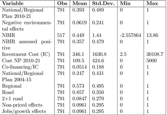
Table 1: Summary statistics for variables included in Model 1. available, the various counties’home pages.
The data set contains 886 projects; we do not have all data available for all objects. Besides, we have deleted observations for which the investment cost variable is missing or takes a value of zero (43 observations); we deem these values to be implausible and the observations to be unuseable. Moreover, we also deleted observations for which a variable ’Prestations to entrepreneurs in 2009’took a value of one (52 observations); this variable indicates projects that were ongoing when the Plans for 2010-2021 were approved of, and there-fore, in a sense, "non-negotiable". Since the transport policy goals discussed in the Introduction only apply since 2009, these projects have been chosen using another criteria and are not relevant to the present study. These two omissions leave us with 791 observations. Table 1 shows summary statistics for variables for which we have data for all transport modes. These are used to estimate Model 1.
The dependent variable, ’ National/Regional Plan 2010-21’, is a binary variable taking a value of one if a project is included either in the National
Infrastructure Plan for 2010-2021, or to one (or more) Regional Infrastructure Plan(s) for 2010-2021, and zero otherwise. The …rst explanatory variable, ’Negative environmental e¤ects’, is a binary variable taking a value of one if the project has negative environmental consequences, above all e¤ects on landscape or noise, and zero otherwise. ’NBIR’stands for the Net Bene…t-Investment Cost Ratio (information included in the CBA and investment cost), and is a variable calculated by the Swedish Transport Administration, where a value greater that 0 indicates that the societal bene…ts from the project exceed the costs. The ’NBIR assessed positive’is a binary variable taking the value one if the civil servants at either the former Road or the Rail administration have made the assessment that despite a missing NBIR, or a calculated negative value, the project in fact has a positive NBIR. We have further set ’NBIR assessed positive’equal to one for those projects that have a reported positive NBIR in excess of 0.2. The choice of this limit is arbitrary. We use variable ’NBIR’in the regressions of Models (a), and variable ’NBIR assessed positive’in Models (b).
We also include a number of …nancial variables, among them ’Investment cost’ (IC), and ’Cost NP 2010-21’, which shows the cost of the project to the present National Plan. This may di¤er from IC because it may be that the project will be …nished after the present plan runs out, i.e., after 2021, in which case not the whole cost falls on the present plan. Besides, the variable Cost NP 2010-21 for natural reasons takes the value of zero for those projects that have not been included in the National Plan. The …nal …nancial variable is the ’Co-…nancing/IC’ variable, indicating the share of co-…nancing by municipalities or private actors of the total IC. The variable takes values between 0 and 1 despite of not being a binary variable, as it indicates the share of investment from other sources than the national and county budgets.
Variable ’National/Regional Plan 2004-15’is a binary variable taking the value one if the project has been included in the previous National or a Regional Plan for years 2004-2015. ’Regional’ is an indicator variable tak-ing the value one for projects on the Regional level, i.e., projects that have been included in, or considered to be included in a regional rather than the
national Plan. These projects are mainly …nanced from a county-level bud-get, rather than the national one. ’Road’ is an indicator variable for road projects, and ’2+1 road’ is an indicator variable for a speci…c type of road projects which are assumed to have considerable tra¢ c safety bene…ts. The "2+1" roads have alternating stretches of three lines, two of which are in the same direction in order to make overtaking easier, and with a separation of the lines from oncoming tra¢ c. Variable ’Non-priced e¤ects’captures in-formation from the civil servants at the Swedish Transport Administration concerning non-priced e¤ects that have not been included in the formal CBA, and …nally, ’Jobs/growth e¤ects’ is a binary variable taking a value of one if it is estimated (by the civil servants at the Swedish Transport Adminis-tration) that the project has a bene…cial e¤ect on job creation or economic growth. Despite the fact that ’Non-priced e¤ects’and ’Jobs/growth e¤ects’ have exactly the same mean and standard deviation, the two variables are not identical but take the value of one for di¤erent objects.
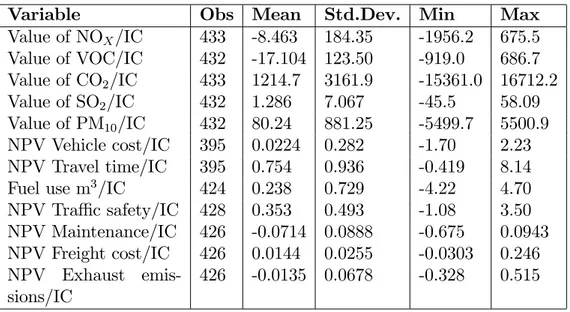
Table 2 summarises variables for which we only have data for road projects. This data, along with the data shown in Table 1 is used to estimate Model 2.
The emission variables (NOX, VOC, CO2, SO2 and PM10 to IC) measure
the change in the value of the given emission in year 2020 to IC, SEK/MSEK. A positive value indicates that the value of the variable (and consequently, emissions) increases, and a negative one that the value (and consequently, emissions) falls if the object is built. For instance, the value of the fall in NOX
emissions for the project that leads to the greatest fall in these emissions is 1956 SEK/invested MSEK, and the value in the increase in NOX emissions
for the project that leads to the greatest increase is 675 SEK/invested MSEK. In order to calculate the value of the change in emissions, we have used the standard values from SIKA (2009). These are shown in Table 3.
NPV in Table 2 stands for "net present value", in MSEK. We have net present value data for a number of project attributes, such as vehicle costs, travel time, tra¢ c safety, maintenance, freight cost and exhaust emissions. The NPV may also be negative (per invested MSEK), as is clear from Table 2. The values of the NPV variables have been taken directly from the
cal-Variable Obs Mean Std.Dev. Min Max Value of NOX/IC 433 -8.463 184.35 -1956.2 675.5 Value of VOC/IC 432 -17.104 123.50 -919.0 686.7 Value of CO2/IC 433 1214.7 3161.9 -15361.0 16712.2 Value of SO2/IC 432 1.286 7.067 -45.5 58.09 Value of PM10/IC 432 80.24 881.25 -5499.7 5500.9 NPV Vehicle cost/IC 395 0.0224 0.282 -1.70 2.23 NPV Travel time/IC 395 0.754 0.936 -0.419 8.14
Fuel use m3/IC 424 0.238 0.729 -4.22 4.70
NPV Tra¢ c safety/IC 428 0.353 0.493 -1.08 3.50 NPV Maintenance/IC 426 -0.0714 0.0888 -0.675 0.0943 NPV Freight cost/IC 426 0.0144 0.0255 -0.0303 0.246 NPV Exhaust emis-sions/IC 426 -0.0135 0.0678 -0.328 0.515
Table 2: Summary statistics for the additional variables included in Models (4) to (8).
Pollutant ASEK 4 value
NOX 36 SEK/kg
VOC 68 SEK/kg
CO2 1.50 SEK/kg
SO2 333 SEK/kg
PM10 11 494 SEK/kg
Table 3: Values of …ve pollutants from ASEK 4 (SIKA, 2009)
culations by the Swedish Road Administration, and divided by IC. Finally, since we do not have data from the Swedish Road Administration for the net present value of fuel use, we have chosen to include the change in fuel use due to the project being built in cubic meters. Nevertheless, we normalise even this variable for the IC.
An analysis of correlations (the table has not been included) between the variables shown in Tables 1 and 2 indicates potential problems with multicollinearity between some of the variables. The correlation between the ’NOX/IC’one one hand and the ’CO2/IC’and the ’SO2/IC’on the other is
0.79 and 0.78, respectively. The correlation between the ’CO2/IC’ and the
’PM10/IC’, the correlation coe¢ cients being 0.81 and 0.85, respectively.
Another variable with high correlations with others is ’Fuel use m3/IC’,
which is correlated with the ’NOX/IC’ (0.80), the ’CO2/IC’ (0.94), the
’SO2/IC’ (0.999), the ’PM10/IC’ (0.85), the ’NPV vehicle cost/IC’ (-0.87)
and the ’NPV exhaust emissions/IC’(-0.98). Also the ’NPV exhaust emis-sions/IC’is correlated with ’NOX/IC’(0.87), the ’CO2/IC’(0.93), the ’SO2/IC’
(0.98), the ’PM10/IC’ (0.84) and …nally, the ’NPV vehicle cost/IC’ (0.85).
These correlations may lead to greater estimates of standard errors of the coe¢ cients, and consequently, to the rejection of the alternative hypothesis when it in fact holds.
4
Results from statistical analysis
Table 4 in Appendix 6 shows the average marginal e¤ects from the estima-tion of Model 1. We do not …nd support for Proposiestima-tion 1 from the results in Table 4. Quite the contrary, the presence of negative environmental e¤ects from a project raises the probability of a project being included in a Plan. Speci…cally, a marginal increase in (the binary) variable ’Negative environ-mental e¤ects’increases the probability of a project being included in a Plan with about 15-20%.5 We have no direct explanation to this e¤ect but suspect
that the variable may capture some other positive, uncontrolled for, e¤ects that the projects with negative environmental e¤ects have, thus acting as a proxy for something.
As for the control variables in both Models 1(a) and 1(b), they fare well and take, for most part, the expected signs. Both the ’NBIR’and the ’NBIR assessed positive’variables are positive and signi…cant at 0.01% level of singi-…cance in both models. In Model 1(a), ’Investment costs’do not matter for the probability of being included in a Plan, while in Model 1(b) the vari-able is borderline signi…cant at 5% level of signi…cance, and negative. Large projects thus have a slighty smaller probability of being included in a Plan 5As Greene (2000, 817) points out, the derivative with respect to a binary variable as
if it were continuous provides an approximation of its marginal e¤ect that is surprisingly accurate.
than smaller projects, the (statistically signi…cant) average marginal e¤ect being of an order of magnitude of -0.004%. Projects with a higher ’Cost NP 2010-21’have a greater probability of being included; we have no explanation to this e¤ect.
A project, which was included in the National or a Regional Plan for 2004-15 has a greater probability of being included even in a "present" Plan, the coe¢ cients being statistically signi…cant at, at best, 0.01% level of sig-ni…cance. This shows that once a project has been included in a Plan, it has a great probability of actually being built, regardless of the other at-tributes of the project. Old priorities thus continue their lives beyond their revision. ’Regional’projects have a greater probability of inclusion in a Plan. Road projects are less likely to be included in a Plan. This is in line with Regeringens skrivelse (2009, 5), where the government states that more rail investments have been included in the plan than was the case in the Road and Rail Administrations’original proposals. Surprisingly, also the 2+1 roads are less likely to be included in a Plan, despite for controlling for roads separately, at, at best, 0.01% level of signi…ciance. The explanation to this may be that the "easiest" and most pro…table 2+1 projects have already been built. It may also be that opposition from certain groups, above all motorcyclists, is playing a part here.
Finally, as expected, the presence of non-priced e¤ects increases a project’s probability of being included in a Plan, the coe¢ cient being signi…cant at 1-5% level of signi…cance, while having a positive e¤ect on jobs and/or eco-nomic growth does not matter in Model 1(a). In Model 1(b), ’Jobs/growth’ lowers the probability of being included in a Plan, the coe¢ cient being signif-icant at 1% level of signi…cance. The marginal e¤ects of the control variables in Table 4 vary somewhat between versions (a) and (b) of Model 1.
We run four versions of Model 2, shown in Table 5. In version (a) we in-clude NBIR as an explanatory variable, but exin-clude the control variables that have been included in the calculation of the NBIR, with the exception of the environmental variables. In version (b) we include ’NBIR assessed positive’ and all the control variables. In version (c) we do not include any measure for the NBIR but examine how the other variables, which are formally
in-cluded in the NBIR calculations, for themselves a¤ect the probability of a project being included in a Plan. In version (d) we exclude three of the highly correlated variables: ’NPV vehicle cost/IC’, ’Fuel use, m3/IC’and ’NPV
ex-haust emissions/IC’ from the regression, and do not include a measure for the NBIR.
The four versions of Model 2 have di¤erent interpretations. From Model 2(a) in Table 5 we can see that the only environmental variable having a signi…cant coe¢ cient at 5% level is ’Negative environmental e¤ects’, which, again, gets a positive sign contrary to our expectation. Other factors having a statistically signi…cant (at least at 5% level) explanatory e¤ect on the probability of being included in a Plan are NBIR, ’Co-…nancing/IC’, ’Plan 04-15’, ’Regional’and …nally ’Non-priced e¤ects’, all of which get the expected positive sign.6 Thus, except for the impact that the emissions variables have
on the probability of being included in a Plan through the NBIR, they do not have any additional impact.
In Model 2(b) we have included ’NBIR assessed positive’instead of NBIR as a control variable, and also included all the other control variables. The ’NBIR assessed positive’variable gets the expected positive sign and is sig-ni…cant at 5% level. Of the environmental variables, ’CO2/IC’ also gets a
signi…cant, at 5% level, average marginal e¤ect and the expected negative sign. Assuming that ’NBIR assessed positive’ captures the planners’ valu-ation of a positive NBIR on the probability of a project being included in a Plan, then they also give additional weight to ’CO2/IC’in their decision.
The only other signi…cant control variables are ’Plan 04-15’and ’Regional’, both with positive signs signi…cant at 1% level.
We left out all measures of NBIR out from model 2(c) in order to get a clearer understanding of which "components" of the CBA that weigh most. The only variable that is included in the CBA and that gets a signi…cant, at 5% level, average marginal e¤ect in the fourth column of Table 5 is the ’NPV tra¢ c safety/IC’, which gets the expected positive sign. Other than that, 6The variable ’Regional’does not have an expected sign as we have no hypothesis about
the ease of building regional projects versus national projects. We accept the signi…cant positive sign as reasonable.
’Plan 04-15’, ’Regional’ and ’Non-priced e¤ects’ all get positive signi…cant signs. The average marginal e¤ect for ’CO2/IC’ is signi…cant and negative
at 10% level of signi…cance (at 6.4% to be exact). It is thus unclear on which components of the CBA that the decision to include in or exclude from a Plan is made.
Finally, excluding the three variables most likely to cause multicollinearity from the regression in Model 2(d), we …nd results very similar to Model 2(c) with the exception of ’CO2/IC’which is signi…cant and negative at 5% level
of signi…cance. We also …nd a statistically signi…cant marginal e¤ect for ’Co-…nancing/IC’, but consider the estimate unreliable because of the huge average marginal e¤ect calculated. The results may possibly be explained as a de…ciency in the data. Otherwise, ’Plan 04-15’, ’Regional’, ’Non-priced e¤ects’ and ’NPV tra¢ c safety/IC’ are again signi…cant and positive, as expected.
We thus …nd some weak support for Proposition 1 from the estimates shown in Table 5. The result only holds for CO2, however, and then when
we do not include NBIR as a variable in the regression. Emissions of CO2
do not get a "second consideration" in decision-making beyond their impact throught the NBIR.
5
Summary and conclusions
We have estimated six regression models to test a hypothesis, namely that environmental concerns a¤ect the choice of transport infrastructure invest-ment projects in Sweden. From the full sample of 791 observations, including both rail, road and maritime projects, we …nd no support for this hypothe-sis. Quite the contrary, it seems that the presence of negative environmental e¤ects raises the probability of a project being built for this sample. The average marginal e¤ect for the variable is about 15-20%.
In order to be able to use more detailed data about the emissions of …ve pollutants (NOX, VOC, CO2, SO2 and PM10), we proceed to estimate
four further equations. This data only contains road investments. When we include NBIR in the regression, we …nd no statistically signi…cant e¤ect
from the pollutants on the probability of being included in a Plan. Only the variable ’Negative environmental e¤ects’ is positive and signi…cant at 5% level, the average marginal e¤ect is about 19%. Using a binary variable which is positive if the NBIR is assessed to be positive instead, or leaving out a measure for the NBIR alltogether, we …nd a statistically signi…cant (at 5-6.4% level) and negative e¤ect for CO2. The average marginal e¤ect
for ’CO2/IC’ is about -0.01%. In other words, a marginal increase in the
variable ’Change in the value of CO2 emissions in 2020 to IC’ around the
average value of the variable (1215 SEK/MSEK) lowers the probability of a project being included in a Plan with 0.01%.
We thus conclude that with regard to NBIR, none of its component bene-…ts or costs gets a weight that is greater than the weight given to the measure of NBIR itself in decision-making. In other words, the environmental factors matter as so far they enter the NBIR calculation. Of the factors entering the NBIR measure, however, there are only two that have a statistically sig-ni…cant e¤ect on the probability of being included in a Plan: the ’Change in the value of CO2 emissions in 2020 to IC’ and the ’Net present value of
tra¢ c safety measures to IC’, both with expected signs. It seems that the other factors’impact on the NBIR is so low that they do not matter at all when decisions about which projects to include in a Plan are made. What matters more is whether a project was included in an earlier Plan (for pe-riod 2004-2015), whether it is a regional project or not, and whether the project has non-priced e¤ects. All these three variables get robustly signi…-cant coe¢ cients. The average marginal e¤ect from the previous Plans (’Plan 04-15’) is about 14% (17% for model 2(a)), that for regional projects is about 21% (30% for Model 2(a)) and that for non-priced e¤ects varies from about 18% (which is signi…cant at 10% level in Model 2(b)) to 28% in Model 2(a) (signi…cant at 0.01% level).
While the present study points at some consideration for the environment, above all emissions of CO2, when transport infrastructure projects are chosen,
it does not explain why the bureaucrats and the politicians care about the environment and want to take it into consideration. A simple explanation to this might be, for instance, electoral concerns if a large share of the electorate
cares about emissions. Building such a model to explain policy choices and, by extension, their impact on project choice, is left for future research.
References
Eliasson, J. and M. Lundberg (2010). Do cost-bene…t analyses in‡uence transport investment decisions? experiences from the swedish transport investment plan, 2010-2021. Number July 11-15, Lisbon. 12th World Con-ference on Transport Research.
Environmental Objectives Secretariat (2010, 11 November). Environmental objectives portal. www.miljomal.se/Environmental-Objectives-Portal/. Greene, W. H. (2000). Econometric Analysis (Fourth international edition
ed.). Prentice Hall International, Inc.
Regeringens Proposition (2009). Mål för framtidens resor och transporter. Prop. 2008/09:93.
Regeringens Skrivelse (2009). åtgärdsplanering för transportsystemet 2010-2021. Nationell plan för Sveriges transportsystem 2010-2021: http://www.regeringen.se/content/1/c6/14/32/32/7c241861.pdf. Ac-cessed 26 August 2010.
SIKA (2009, 19 October). Samhällsekonomiska principer och kalkylvärden för transportsektorn: ASEK 4. Technical Report 2008:3, SIKA.
SOU (2010). E¤ektivare Planering Av Vägar Och Järnvägar. Stockholm: Fritzes. SOU 2010:57.
6
Appendix
Nat./Reg. Plan 2010-21 Model 1(a): av-erage marg. e¤.
Model 1(b): av-erage marg. e¤.
Neg. env’l e¤. 0.201** 0.151*
(2.63) (2.18)
NBIR 0.0576***
(4.02)
NBIR ass. positive 0.194***
(6.25) Investment Cost -0.0000358 -0.0000444* (-1.31) (-1.96) Cost NP 2010-21 0.000330*** 0.000196** (3.33) (2.92) Co-…nancing/IC 0.658*** 0.722*** (4.42) (5.69) Plan 2004-15 0.108** 0.130*** (2.74) (4.10) Regional 0.262*** 0.191*** (4.67) (4.67) Road -0.333*** -0.432*** (-4.33) (-8.55) 2+1 road -0.242*** -0.195** (-3.43) (-3.04) Non-priced e¤ects 0.185* 0.181** (2.48) (2.86) Jobs/growth -0.0956 -0.151** (-1.36) (-2.65) Observations 517 791 z statistics in parentheses * p<0.05, ** p<0.01, *** p<0.001
Table 4: Regression results for Model 1; with NBIR as an explanatory vari-able in 1(a) and with NBIR Assessed positive as an explanatory varivari-able in 1(b).
Nat./Reg. Plans 2010-21
Model 2(a) Model 2(b) Model 2(c) Model 2(d)
NOx/IC 0.000100 0.000366 0.000380 0.000159 (0.50) (0.47) (0.47) (0.39) VOC/IC -0.000125 -0.000575 -0.000667 -0.000233 (-0.49) (-1.25) (-1.43) (-0.81) CO2/IC -0.0000158 -0.000162* -0.000129 -0.000149* (-0.93) (-2.25) (-1.86) (-2.00) SO2/IC -0.000683 0.470 0.593 0.140 (-0.12) (1.00) (1.25) (1.89) PM10/IC 0.000052 7.87 10 6 -2.86 10 6 0.0000113 (0.99) (0.13) (-0.05) (0.20)
Neg. env’l e¤. 0.192* 0.0460 0.0582 0.0719
(2.32) (0.50) (0.62) (0.76)
NBIR 0.0576**
(3.29)
NBIR Ass. Pos. 0.127*
(2.21) Investment Cost -0.0000625 0.0000482 0.000021 0.0000191 (-1.84) (0.52) (0.23) (0.21) Cost NP 2010-21 0.000277 0.000413 0.000452 0.000429 (1.90) (1.60) (1.68) (1.64) Co-…nancing/IC 0.514** 30.8 31.2 133.2*** (3.48) (0.03) (0.03) (24.00) Plan 04-15 0.168*** 0.149** 0.145** 0.143** (3.85) (3.47) (3.36) (3.28) Regional 0.302*** 0.214** 0.218** 0.211** (5.00) (3.14) (3.18) (3.10) Non-priced e¤ects 0.283*** 0.177 0.215* 0.230* (3.50) (1.93) (2.34) (2.53) Jobs-Econ. Growth 0.0697 0.149 0.170 0.157 (0.71) (1.50) (1.70) (1.57) NPV vehicle costs/IC -0.0909 -0.0463 (-0.45) (-0.23) NPV travel time/IC -0.00528 0.0311 0.0339 (-0.10) (0.61) (0.77)
Table 5: Average marginal e¤ects for Model (2) with di¤erent speci…cations of control variables.
Model 2(a) Model 2(b) Model 2(c) Model 2(d)
Fuel use, m3/IC -1.37 -1.92
(-0.80) (-1.11) NPV tra¢ c safety/IC 0.0593 0.105* 0.107* (1.06) (2.03) (2.09) NPV mainte-nance/IC -0.189 -0.137 -0.214 (-0.59) (-0.42) (-0.69) NPV freight/IC 2.70 2.65 1.086 (0.86) (0.84) (0.43) NPV exhaust emiss./IC -3.42 -3.79 (-0.92) (-0.99) Observations 430 391 391 392 z statistics in parentheses * p<0.05, ** p<0.01, *** p<0.001