School of Innovation Design and Engineering
Västerås, Sweden
Thesis for the Degree of Bachelor in Computer Science 15.0 credits
SUPERVISED MACHINE LEARNING
(SML) IN SIMULATED ENVIRONMENTS
Mattias Rexby mry17001@student.mdh.se
Examiner: Mobyen Uddin Ahmed
Mälardalen University, Västerås
Supervisor(s): Prof. Ning Xiong
Mälardalen University, Västerås
Abstract
Artificial intelligence has made a big impact on the world in recent years, and more knowledge in the subject seems to be of vital importance as the possibilities seems endless. Is it possible to teach a computer to drive a car in a virtual environment, by training a neural network to act intelligently through the usage of supervised machine learning? With less than 2 hours of data collected when personally driving the car, I show that yes, it is indeed possible. This is done by applying the techniques of supervised machine learning combined in conjunction with a deep convolutional neural network. This were applied through software developed to interact between the network and the agent inside the virtual environment. I believe the dataset could have been cut down to about 10 percent of the size and still achieve the research goal. This shows not just the possibility of teaching a neural network a good policy in stochastic environments with supervised machine learning, but also that it can draw accurate (enough) conclusions to imitate human behavior when driving a car.
Contents
1. Acknowledgements 1
2. Introduction and overview 2
2.1. Presentation . . . 2
2.2. Overview of the Results . . . 2
3. Background 3 3.1. Terminology . . . 3
3.2. General background . . . 5
3.3. The norm of testing . . . 6
4. Related Works 7 4.1. Supervised learning . . . 7
4.2. Reinforcement learning . . . 7
4.3. Reinforcement and supervised learning combined . . . 8
4.4. Supervised learning and Mario Kart 64 . . . 8
5. Problem Formulation 9 6. Method 10 6.1. Proposed working procedure . . . 11
6.2. Research method . . . 11
6.3. Experimental work description and reasoning/evaluation . . . 12
6.3..1 Setting up virtual environment . . . 12
6.3..2 Capturing image and action . . . 12
6.3..3 Data collection and paring . . . 12
6.3..4 Creating the neural networks . . . 13
6.3..5 Normalizing, balancing and training . . . 13
6.3..6 Software for testing the model . . . 14
6.3..7 Testing and evaluating the model . . . 14
7. Research ethical considerations 15 8. Process and applied techniques 16 8.1. Experimental setup . . . 16
8.2. Creating the dataset . . . 17
8.3. Creating the Convolutional neural network . . . 17
8.3..1 Convolutional neural network model structure . . . 24
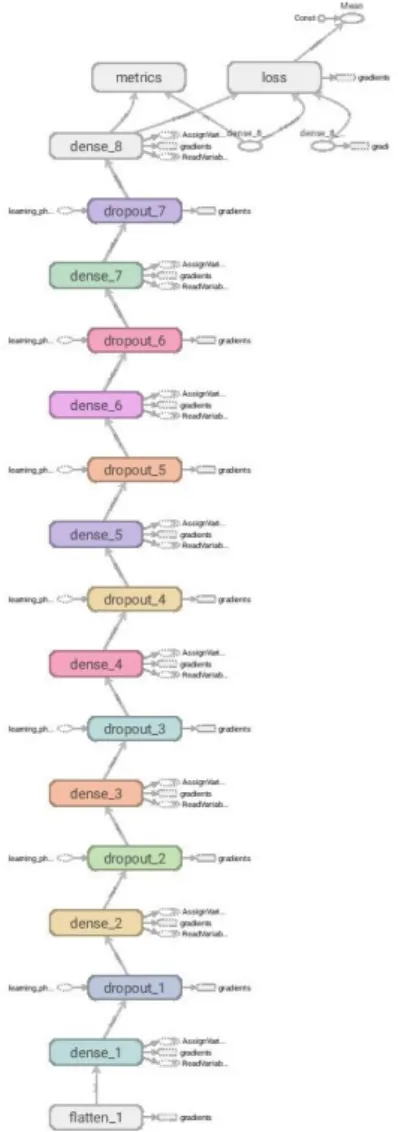
8.4. Creating the Neural network . . . 25
8.4..1 Neural network model structure . . . 25
8.5. Loading the data . . . 25
8.6. Normalizing the data . . . 25
8.7. Balancing the data . . . 26
8.8. Training the model . . . 26
8.9. Testing the model . . . 26
8.10. Evaluating the model . . . 27
9. Results 28 9.1. Convolutional neural network . . . 28
9.2. Neural network . . . 29
9.3. Analysis . . . 30
9.3..1 Convolutional neural network . . . 30
9.3..2 Neural network . . . 30
9.4. Comparison between techniques . . . 30
9.4..2 Supervised learning and Reinforcement learning . . . 31
9.4..3 Supervised learning combined with reinforcement learning . . . 31
10.Discussion 34 10.1. Research question evaluation and scientific discussion . . . 34
10.1..1 Reflections and consequences . . . 34
10.2. Reinforcement learning and image classification . . . 35
10.3. Ethical and social considerations . . . 35
10.3..1 Social consequences and economic considerations . . . 35
10.3..2 Legal considerations . . . 36
11.Conclusion and significance 37 12.Future works 38 12.1. General considerations . . . 38
12.2. Reliability and dataset reduction . . . 38
12.3. Cyber attacks . . . 38
12.4. Adding actions and complexity . . . 38
12.5. Supervised and reinforcement learning . . . 39
12.6. Incremental applications . . . 39
List of Figures
1 Neural network. From [7]. CC-BY . . . 3
2 Calculate screen coordinates . . . 16
3 Convolution 2D. From[75]. CC-BY . . . 17
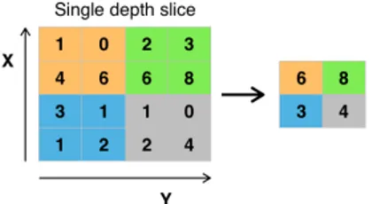
4 Max pooling. From[78]. CC-BY . . . 17
5 Dropout. From[79]. CC-BY . . . 17
6 Rectified Linear Unit (ReLU) - Activation function. From[80]. CC-BY . . . 18
7 Padding the Convolutional layers. From[81]. CC-BY . . . 18
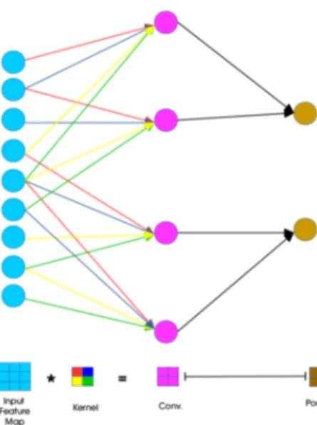
8 Convolution on feature map. From[83]. MIT . . . 19
9 Softmax activation function. From[84]. CC-BY . . . 19
10 Prediction class and Estimate error . . . 20
11 Stochastic Gradient Descent (SGD) versus SGD-Momentum (SGDM). From[87]. GNU GPL . . . 22
12 Pixel effect on weight update in convolutional layers. From[88]. MIT . . . 23
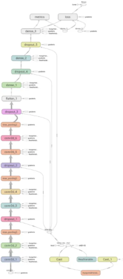
13 Tensorflow representation of the convolutional network structure - only including vital information . . . 24
14 Tensorflow representation of the neural network structure - only including vital information . . . 25
15 Testing with different settings - accuracy graph . . . 26
16 Mario gets stuck entering the tunnel . . . 28
17 Mario gets stuck going thru the tunnel . . . 28
18 Mario completing the research goal . . . 28
19 Mario driving on a track never seen before . . . 29
20 Neural network. Orange = training accuracy/loss, blue = validation accuracy/loss 29 21 CNN - Confusion matrix, precision, recall, f1-score: in percentage . . . 32
22 NN - Confusion matrix, precision, recall, f1-score: in percentage . . . 33
1.
Acknowledgements
I would like to thank my supervisor, Professor Ning Xiong. For making time in his busy schedule to act as my supervisor, guiding and helping me to navigate the complicated world of research. Further I would like to thank him for encouraging me to not just write a thesis. But also to do it in a way where I can take pride in the work done and how it is presented.
2.
Introduction and overview
2.1.
Presentation
Recent breakthroughs in machine learning have made it possible to innovate in fields like self-driving cars, autonomous machines and spell checking, etc. The purpose of this work is to further improve general knowledge and understanding about the ability of supervised machine learning[1] implemented thought deep convolutional neural networks[2] to learn a good policy and generalize well in stochastic environments. I used approximately 2 hours of data collection for this experi-ment. Where as in 2106 Nvidia[3] used about 72 hours of data collected. In a similar but more advanced research in 2017, Kinsley[4] used more than 33 hours of video, teaching an agent to play Grand theft auto 5 with supervised learning implemented as a convolutional neural network. He recommended that at least 1 million images were to be collected (approximately 33 hours of video collection and about 125,000 images per class, equivalent to about 4 hours of footage per class). Where preferred to get good generalization in the model. However he later stated[5] that the new updated dataset where huge, indicating that much more than the previously mentioned 1 million images was collected. The motivation behind the thesis comes for studies like these, which requires huge investments in time when collecting data to draw from and introduces a hindrance in terms of being able to conduct research in the area as the collection needs to be conducted before any work can begin. I aimed to severely cut the size of the dataset by focusing on generalizing the data, rather than focusing on gathering huge amounts of data. The idea was that two pictures of the same thing will not reinforce the learning policy, but instead make the model biased to that class introducing bad generalization. The questions being evaluated are: How can a convolutional neural network agent be trained to complete 3 consecutive laps on "Luigi highway" in Mario kart 64 under 5 minutes with less than 120 000 image/action pairs to train from, and no external sensors applied? and. How is it possible to complete 1 lap on any of the other (previous unseen) tracks in Mario kart 64 with the same model?
2.2.
Overview of the Results
The results exceeded my expectations and the overall conclusion was that the research were a success. The agent successfully learned to stay on the track with just 20 min of data collected (approximately 20 000 images). However it did not generalize well enough to complete the research goal and often got stuck on the track. This was probably due to the poor diversity in the data collected, since all the images were gathered from the same track. By extending the dataset to 115 000 images, the agent did not just complete the track. It were also able to generalize and learned a good policy. Furthermore it was able to complete several other tracks as well and even tracks never before shown to the agent. The agents were generally unable to perform at an adequate level whenever it left the road. Also it was unable to solve problems of getting back on the track and wasn’t able to distinguish from going the right or wrong way on the track. These problems were likely due to not receiving any data showing a human solving these kinds of problems. Introducing such data would however likely also introduce more noise to the model and diminished the overall performance of the model. Using data like that meanwhile continuing to keeping it small, would have forced me to change "good" data for data handling special chases. It would likely not have been preferred to the way I did it, as the model already showed problems with generalization due to the data being too sparse. This was a hypothesis I had and because of this hypothesis, I did not chose to include such data in the dataset.
I show in the research that the agent could generalizes well and was able to make accurate enough predictions on tracks which it has never seen before. This gives us some general knowledge about the bigger need for diversity in datasets, rather than the size of the dataset (in terms of more images). The reason for doing research in this area is the idea that it yields important information for supervised learning and neural networks in general[6]. It also increases the common under-standing and helps with the decision-making when deciding how to implement neural networks in machine learning. This can have major impacts in for example industries including but not limited to; medicine, transportation, video games, infrastructure, logistics, etc.
3.
Background
3.1.
Terminology
In this section I discuss in short some terminology and concepts used in the report which is essential to grasp in a general sense to understand this research in the field of machine learning with neural networks. In the report the terms, "supervised learning" and "supervised machine learning", will frequently be interchanged. But in this field discuss about supervised learning, generally referees to supervised machine learning[1].
Figure 1: Neural network. From [7]. CC-BY Artificial neural network[8] - The
inter-connection of layers with nodes. The lay-ers can have a varying size, but not more than one hidden layer Figure 1". A good analogy is the human brain which the idea of artificial neural networks is derived from[9]. In this report the terms artificial neural net-work and neural netnet-work will be interchanged frequently as they are the same, only with the difference of one being artificial (non tan-gible).
Artificial deep neural network[10] - It is a neural network with at least two hidden lay-ers, the amount of layers can theoretically be infinite. The picture in Figure1", shows two fully connected neural networks. Meaning all the nodes in each layer is connected to all nodes in the layer before and the layer after, this is not always the case.
Node in neural network[11] - The node is a unique value, decided by the path of the in-formation traveled there. Each node has a weight and bias associated with it. The weight is a scalar value which changes as the model trains, with the calculated error between prediction and classification of the training data. The bias can be described as, a non zero figure. It is used to remove the possibility for nodes to have a zero value, which renders them dead or unusable. Furthermore, it’s also used to help the model fit to nonlinear data. Ultimately these are what creates the policy of the model together with the rest of the nodes in the network.
Hidden layer[11] - The hidden layers are one or more nodes in between the input and out-put layers of a neural network. Example: The right network in Figure1has 2 hidden layers.
Exploding gradients[12] - The network can in some cases suffer from exploding gradients. It is a term used when the number applied to a node is too big and a "inf" (short for infinity) status is instead applied. This renders the node and ultimately the network useless, it is also called a dead neural network[12].
Overfitting[13] - Overfitting a network is when the weight and biases are tuned to only make accurate predictions on data in the training dataset, and it does not generalize well outside the training data.
Pruning[12] - Pruning is when hidden layers are removed or decreased in size. To lessen the possibility of overfitting. The reason of pruning a model is to force it to generalize better when doing predictions.
State/observation space[14] - It is the information which the neural network receives as an input. It’s a representation of the world to which the network is supposed to find unique features. It will then be able to distinguish different data in the state from each other. It can vary and be things like images, measurements and sound waves etc.
Class/label[10] - The information provided to a neural network about what it is currently see-ing. The classification is a numerical representation of what we want the neural network to learn. Example 0 = dog, 1 = cat, 2 = bird, and so on. When the network predicts the wrong figure it updates weight and biases through the mathematical procedure of backpropagation. This improves the likelihood of the correct prediction being made next time the image is presented to the network.
Supervised learning[1] - The subfield of machine learning called supervised learning, is the general term for teaching a neural network a policy by forwarding information about a state paired with the classification of the state. The neural network outputs a prediction which is a numerical classification of the state, and compares this prediction against a label/classification provided with the state. The label is however not forwarded through the network. The potential error in this prediction versus the label is used to update the weights and biases of the neural network with backpropagation[15], resulting in better predictions and smaller errors in the future.
It is more clearly defined as the way of providing the network with the state, and at the same time giving information about what the state is representing. The information which the network receives will be the base for the prediction and the label is what to compare the prediction against. It can be an image, but it can also be a numerical representation of data. For example measure-ments of different flowers like the Iris dataset[16], where the network will learn to associate the measurements with the appropriate flower.
Unsupervised learning[17] - Is also a subfield of machine learning, where the agent learns to recognize similarities and differences in data without any other information then the observation space provided. It is often applied in medicine where most of the information is identical and the important information is found in the differences, not in the similarities in a regular sample. It is also applicable in supervised learning to recognize noise in the data. By extracting as much information as possible from a given dataset while using the smallest number of futures, we can save significant computing time and often build models that generalize better to unseen data.
Reinforcement learning[18] - The subfield of Machine learning that is called reinforcement learning, learns inside an environment through trial and error. The agent is provided with a state inside a predetermined context of an environment and then receives a reward for the action taken. The action is chosen by passing the state into a neural network and receiving a prediction on what action to take. The reward is based upon the state which is received by taking the action and also a discounted maximum possible future reward, which is possible to reach from this new state. This teaches the agent by trial and error[19] a good policy by associating good and bad action pairs. The goal is for the agent to maximize the total reward, each round.
Reinforcement learning is often used in industries to learn or improve the movement on for example robotic arms[20] and alike. This field of machine learning creates the possibility for machines to learn good or even optimal policies by giving them some reference values received as rewards. Where there is no need for the machine to know anything about the observation space beforehand. Usually the equations used for reinforcement learning are variants of the Bellman equation. Sample of reinforcement learning equations:
Deterministic equation: Q(s,a) <- ra
s0s+ ymax(0a)Q(s0, a0)
Stochastic equation: Q(s,a) <-Q (s,a) + α[ra
s (0s)+ ymax(0a)Q(s0, a0) − Q(s, a)]
Where:
s = State Q = Q-value for state/action pair a = Action k = Times the state has been visited k = Times the state has been visited r = Reward for action
3.2.
General background
Machine learning was first introduced and proposed by Hebb[21] in 1949. He also described the mechanism of "neural plasticity" which today is called unsupervised learning[22]. This was the first proposed technique for implementation of artificial neural networks. In later years more im-plementations of artificial neural networks have been proposed and researched. One of these is supervised machine learning[1] in the form of a convolutional neural network[2], which relies on the previous collection of labeled data. It uses the collected data as training samples where it tries to predict what classification is represented in the image, and the error in the prediction is used through the mathematical procedure of backpropagation[15], to update the weights and biases to give better predictions in the future. In 2009[23] the technology of utilizing parallel GPU-processing in implementations of machine learning was proposed and available for commer-cial usage. This made it possible for several breakthroughs to be made and new ways of using neural networks were tested, which have since evolved at an accelerated rate[24]. For example, an reinforcement learning[18] task that needed 384 systems with a total of 6144 CPU-cores and 8 Volta V100 in 2019[25], can one year later be done in 1/3 of the time on a single A100 GPU[26]. This shows just how fast innovation in the area is progressing. Another example of breakthroughs is, AlexnNet[27] which was created to categorize 1000 classes of images at a super-human level. In addition, DeepMinds[28] implementation of reinforcement learning to beat all of the Atari 2600 games at a super-human level. There are more industrial fields like spelling checking, language translation, pattern classification[29], medical innovation[30] and sound synthesis that have had astonishing effects applied to them through machine learning.
Improvements done in this area are vast and rapidly advancing. We have self-driving cars and face recognition on phones. DeepMind reports an energy saving beyond 40 percent[31] on Google’s server-centers due recent breakthroughs in machine learning. More research in these areas seems to be of great interest and importance to many industries. A recent study from McKinsey Global Institute suggests that by 2030, intelligent agents and robots could replace as much as 30 percent of the world’s current human labor[32]. These kinds of studies highlight the importance and impact of machine learning in the society.
In recent years several benchmarks for testing neural networks have been constructed. For the explicit reason of testing and measuring the performance of a neural network, making it easy to do comparisons between different models. For example the ImageNet’s benchmark where one is to categorize 1.3 million images with 1000 categories of things[33], ranging from dogs and cats to airplanes and pencils. The measurement of performance is the accuracy measured on out of sample data which is kept from the model until the training is concluded. There is also the Iris data classification benchmark[16], where several numerical measurements on flowers are used as inputs. This teaches an agent to predict the type of flower by associating the different measurements with types of flowers. These types of benchmarks have with time been somewhat outdated due to the improvements made in understanding neural networks, and new benchmarks have been proposed. One reason for this is that what was impressive in 2012 is not so competitively impressive today. For example AlexNet 2012 with 84,2 percent correctness in the ImageNet challenge, which was 10.8 percent better than the runner-up[34], is today far behind as in the most recent ImageNet competition the difference between the first and the fiftieth participants were 5,21 percent and all of them were better than AlexNet.
Lately more and more benchmarks have been created in stochastic game environments. Where the uncertainty of the opponents move introduces new obstacles for the network to learn. The pro-gression in this field has been astounding. In 2016 Deep Mind mastered the game of AlphaGo[35] and beat the current world champion with a neural network only trained through reinforcement learning. Alpha-Go is supposedly one of the most advanced board games ever created, due to the huge amount of possible moves. In 2019 DeepMind again made a breakthrough. Training an reinforcement agent to master the computer game Dota 2[36]. In this environment the agent had to contest against several opponents at once and work together with several implementations of itself to make a winning strategy. This achievement promoted this quote by Bill Gates. "That’s a
big deal, because their victory required teamwork and collaboration – a huge milestone in advancing artificial intelligence - Bill Gates."[37].
The most recent and possibly the most impressive accomplishment yet in machine learning as a whole, is the successful combination of reinforcement learning[18] and supervised learning[1] used by DeepMind to master the game of Starcraft 2[38][39]. Where the observation space and the action space counts in the thousands creating millions of state/action pairs to keep track of. This achievement showed the benefits of combining reinforcement learning and supervised learning to complete tasks before this, thought to be near impossible. This is due to the time it would take for a reinforcement learning agent to explore all possible states, and the inherently fundamental problem of supervised learning to surpass the performance of the data it is trained on[40].
3.3.
The norm of testing
Testing machine learning systems inside a virtual environment, have become somewhat of an industry standard[41]. This is largely due to several reasons, one of which is the uncertainty of what will be produced after training a neural network, as the policy’s learned is hard or near impossible to accurately predict as the policy is a collection of all the outputs from all the nodes in the networks which is often millions of parameters[42]. Testing inside a virtual environment is a safe and competitively cheap way to see what and how a network learns. Later one can make conclusions about the network and start applying it in real-life situations. The result of training a neural network with some specific data can be theorised about. However giving a 100 percent accurate prediction one would have to conduct extensive mathematical studies, with all potential involving variables included. Which it is often hundreds of millions of mathematical operations to be preformed[42] in larger networks. Every project produced and published in this category reinforces and improves the general knowledge about how and why they work. It also helps us understand how they are most effectively trained and structured. This also creates more empirical evidence for proof-of-concept. Often can a system rigidly tested inside a virtual environment, directly be applied in real life events[43] and perform at acceptable, required or even astonishing levels. This saves time and money when building or/and testing equipment and handling issues raised from accidents and similar situations. Incidents are a not uncommon when handing over controls of machines and things to a computer program before it is rigorously tested and ready[44]. General practise in supervised learning with convolutional neural networks is to collect data in the environment which the system is supposed to work in. Then train the model using most of that data. When the model is complete the model is tested on validation data, which until now is unseen. This will show the performance of the model one can expect in a real-life application, making it easier to predict the behaviour of the model.
4.
Related Works
4.1.
Supervised learning
Nvidia[3] successfully created a self-driving car 2016 by only utilizing supervised machine learn-ing[1]. They did it by implementing a deep convolutional neural network[45], they collected the data required, by a camera on the vehicle which captured images and paired them with the angle of the steering wheel. The model was then trained on the captured data and later tested as an autonomous self-driving car system. This were an extraordinary show of proof of concept, that a neural network has the ability to learn nonlinear policy’s with supervised learning, in real-life situ-ations. Nvidia realized this by collecting about 72 hours of footage and used the pictures and state of angle were used as labeled data to train an supervised learning agent to output a prediction, for the angle of the steering wheel while driving. This was with good enough accuracy for the car to stay on the road when the system was tested. Showcasing this implementation of supervised learning was important for the research community. It essentially showed that research and testing done, inside a virtual environment can be successfully implemented in a real-like setting. This is one of many projects that increased the interests in the research community. To do more research into the usage and possibilities of supervised learning, to teach artificial intelligence to actively interact with the environment through deep convolutional neural networks.
4.2.
Reinforcement learning
In later years reinforcement learning[18] seems to be one of the most promising fields of research in machine learning. This is largely due to the possibility for a computer to compute these kinds of problems at an accelerated rate[46]. This makes problems which before were too complicated to solve, to be within reach nowadays within an acceptable time-frame. Instead of a human running tests and tuning parameters for hundreds or thousands of years, a modern computer can do it in the range of days, -weeks or months, making it a promising field of research in machine learning[38]. Reinforcement learning was used by Ho, Ramesh and Torres Montano[47], to successfully teach an agent to play Mario Kart 64[47]. The project implemented a modified Bellman equation, referred to as the stochastic q-learning equation, to update the weights and biases in their neural network. In real-life implementations teaching an agent a policy through reinforcement learning requires an action space where the agent can do no harm, as implementing reinforcement learning in for example a car would have it crash thousands or millions of times before a policy which would be suited for the general road to be found[19]. Even in situations where reinforcement learning is applicable, one of the most limiting factors is the size of the observation space. When it gets too large it requires computational power, which we of today do not possess. Attempts to utilize reinforcement learning for these kinds of tasks, would result in many years of training before the model would converge. What works well in a virtual environment as Mario Kart 64, would likely be infeasible to reproduce in a simulator depicting real-life. This is due the huge amount of data the model would have to compute to capture all vital information for it to learn a good policy. It is one of the main reasons why reinforcement learning still is not used for such applications. An attempt was done by Kinsley[48] to teach an agent to dive through reinforcement learning in a simplified simulator called Carla[49]. Even when utilizing high-end hardware as the Lenovo p920 workstation, he was unsuccessful in showing any good results. With more advanced hardware it might have been possible for the agent to converge. However the simulator is still just a simplified reality driving simulator which still severely limits the number of variables in an environment where the difficulty is measured by the number of variables. With all variables active including everything that it implies, I do not believe that it is possible to teach an agent to drive a car inside such simulation or in real-life with current hardware, if some limits on training time are enforced.
4.3.
Reinforcement and supervised learning combined
In January 2019 DeepMind[38], made a groundbreaking implementation of machine learning. They were able to beat two of the worlds best players in the strategy game Starcraft 2[39]. It has thou-sands of observations in its observation space and thouthou-sands of possible actions to output, creating millions of possible state/action pairs. One of the main reasons for success were the combination of supervised learning[1] and reinforcement learning[18]. Where the initial exploration face of the reinforcement learning agent, was replaced with supervised learning. The agent managed to get to Damion level performance which is third highest rank in the game, by only training with su-pervised learning. This removed a lot of the initial exploration time for the reinforcement learning algorithm, as it now only needed to perfect the already good policy instead of starting with 100 percent random actions.
The successful combination of supervised learning and reinforcement learning, opened many new possibilities. Areas where conventional reinforcement learning was impractical to implement, due the vast requirements in computational resources. Such areas were now shown to be accessible through the combination with supervised learning, which could shorten the time requirements for convergence by magnitudes. This by teaching the agent a policy with supervised learning first and then just improving the techniques with reinforcement learning. Effectively skipping a huge part of the initial exploration time. Noteworthy is that for DeepMind’s agent to successfully beat the top players. The agent after being trained on supervised learning, still had to do over 200 years of subjective game time with reinforcement learning to converge to that level of performance[38].
4.4.
Supervised learning and Mario Kart 64
Applying supervised learning to play Mario kart 64[47] were successfully done 2016 by Hughes[50]. The scientific aspects of the project can be questioned, as the information was limited. The results were presented as "AI was able to drive the majority of the simplest course"[50]. It does not entail enough information about performance to make any conclusions about exactly what this involves, or the explicit meaning of the statement. The difference between the work done by Hughes and this research, is mainly the scientific approach of the problem. Where as he did not publish any scientific experimental information or stipulated conditions for the goal and success of the project. This research will on the other hand follow scientific guidelines, which creates the possibility for repeatable experimental testing, for more reliable conclusions to be drawn.
Achieving this goal sheds some light on what data is needed to teach a supervised agent a good policy. This might give other applications the possibility to take advantage of supervised learning even though the amount of data is hard and/or time consuming to get. And further reinforces the idea (referring to the previous discussed study, on combinations on reinforcement and supervised learning made by deep mind on Starcraft 2[38][39]) that, time can be saved by implementing su-pervised learning with even just little amount of data first, which can give a good enough policy for a reinforcement algorithm to save time for convergence when exploring the states.
5.
Problem Formulation
Training agents in virtual environments is often the first step on the road to applying the techniques in a real-life setting[43, pp. 8973-8979]. Showing proof of concept brings us ever closer to real-life applications were machine learning using these kinds of techniques can be performed. The purpose of the research was to create a neural network capable of driving a car in a virtual environment. The system will be tested inside the virtual environment Mario Kart 64[47], with the goal of completing 3 consecutive laps, in Mario Kart 64 "Luigi highway" under 5 minutes without human intervention or external sensors applied. In addition complete 1 lap on any previous unseen track. This is to be done through using supervised machine learning[1], where image and action pairs[3] was forwarded to a deep convolutional neural network as training samples. The training where to be done with a small dataset (less then 120 000 images which is about 2 hours of play time or 90 laps on an average track at 30 frames per second). The data was collected on several different tracks in the game, with the expectation of creating a diverse dataset and achieving a good general policy. The purpose of the experiment is to explore if convolutional neural networks[2] can be implemented as a supervised machine learning technique, to solve the complex problem of driving a car in a simulated environment, collecting training data only thought watching a human playing the game. Therefore the research question are:
1. How can a convolutional neural network agent be trained to complete 3 consecutive laps on "Luigi highway" in Mario kart 64 under 5 minutes with less than 120 000 image/action pairs to train from, and no external sensors applied?
2. How is it possible to complete 1 lap on any of the other (previous unseen) tracks in Mario kart 64 with the same model?
The assumption made is that without a trained network which predicts what actions to take, the agent would not be able to complete 3 consecutive laps under 5 minutes.
With a success in terms of goal reached, this project can bring more general knowledge to the field of supervised machine learning. It can also help the general understanding in the inner workings of neural networks. In addition it can assist when applying for funding, to more substantial projects with real-life applications. By showing successful applications using these techniques inside virtual environments. The limited dataset will further help investors to see profits, whereas when costs go down for collecting and storing data, the utilization of the techniques becomes more feasible.
6.
Method
Initially were a literary study conducted including the review of relevant scientific articles and publications within the area of research. The literary study was done to gather a fundamental understanding about the techniques behind neural networks[6], machine learning[1] and convo-lutional neural networks[2]. Furthermore the literary study increased my knowledge about the mathematics behind the algorithms implemented when testing the hypothesis. Through the study of the mathematics which was needed in the creation of the neural network model, I was able to reliably implement a network structure, suited for the problem to be solved. The literary re-view ([1][2][3][4][29, pp. 34–38][30, pp. 706-710][38, pp. 350–354][43][50][51, pp. 809-818][52, pp. 20–29]) suggested/indicated that a supervised machine learning[1] technique utilizing convolutional neural network[2], with techniques as pooling[53], max-pooling[53], dropout[54], ReLU activation function[55] and Softmax activation function[55], was suited to test the hypothesis.
6.1.
Proposed working procedure
The convolutional network structure applied to test the hypothesis can be revived in The process and techniques applied network section. The fundamental motivation behind using the proposed network structure and software implementation can be reviewed in The process and techniques applied. I will give an overview of the reasoning in this section to better understand the method and it’s motivations. The working procedure consists of tree parts. Part 1 is the handling of actions and states through saving the action in a 1-dimensional array paired with the 2-dimensional picture present, when the action was taken. Furthermore the software needed to forward the prediction from the network back into the game environment so the model could be tested in real-time. Part 2 of the working procedure was the convolutional neural network, which was trained separately from the data collection. Part 3 testing the working procedure by forwarding images to the net-work which outputted a prediction for the software to use as an action inside the game. The full software description can be found in section 6.3 and further evaluated in section The process and techniques applied.
Algorithm 1: Proposed algorithm
Result: Network trained and able to forward predictions and implement them in the game environment.
if Collecting data then if New frame then
Save image and action in to a tuple as a (2D-numerical array,1D-binary array); end
if 1000 image/action pairs are collected then Save to hard-drive;
end end
if Training network then
while Validation loss decreasing do Load image/actions from hard-drive; Forward image/action pairs to the CNN; Use 20 % of the data as validation samples;
Backpropagate the error estimation and update weights and biases; end
end
if Testing the network model then while time < 300 do
Forward screen image to network;
Receive action prediction from network by using numpy.argmax on the outputs; Decode action to resemble a keyboard key press;
Preform proposed action in game; end
end
6.2.
Research method
When evaluating the research question the hypo-deductive method was chosen as described in Säfsten och Gustavsson[56, pp. 46-48]. The method chosen is suited where the results are possible to be falsified. Not being able to falsified the results does however not prove that the it is not possible as there can still be situations where it is not cohesive. It will just answer if the research question is verified or not for this specific case. In this experiment it was possible to verify if the agent was able to finish the proposed track under the allotted time limit. It were measured with the in game clock and the game itself informs if and when the goal state was achieved. In trying to evaluate the hypothesis, I implemented a convolutional neural network[2] (network structure and settings in appendix). The network was trained on 120 000 image samples captured together with
the action performed at that time, while I was personally playing the game. This was done by utilizing software I created for the purpose of capturing the image from the screen and paired it with the action taken at that time. The convolutional neural network implementation was done with the API Keras[57] which is a deep learning library, used for software implementations of artificial neural networks[6][8]. The networks weights and biases was updated through the mathematical procedure of backpropagation[15]. It was intended to create a (intelligent) policy for the agent to use when forwarding images to the network to get a prediction on what action to take. The trained network was then able to output a prediction on what action to be performed at each game state. It was used to calculate the error in the action prediction from the network, and later used to perform the action in-game when testing the model against the research question. The in game testing was done by using software which pushed the key-representation of the action predicted from the convolutional neural network. This software was constructed by me for the explicit reason of letting the network dictate what actions to take. Further the network will be measured with k-fold cross validation[58], f1 score[59], ROC curve, confusion matrix[60], precision/recall[61] and compared to the results of a traditional Neural network[6]. However balanced accuracy[62] will not be considered as the classes will be in perfect balance prior to the training procedure (as explained in section 6.3..5).
6.3.
Experimental work description and reasoning/evaluation
This is a work description and reasoning around the choices made. An detailed experimental setup and network description can be found in the section The process and techniques applied.
6.3..1 Setting up virtual environment
First I setup a virtual environment on Windows 10 with a Mario kart 64[63] emulator adapted from Nintendo 64. The keyboard works as a substitute for the original Nintendo 64 controller sending commands from the user to the environment. The emulator chosen was the 640x480 resolution variation. The reason for using the 640x480 resolution variant was that it were easier for a human agent to see what were on the screen when collecting training data than it would be with smaller resolution.
6.3..2 Capturing image and action
I created software which captured the screen image and resizes it from 640x480 to 200x165, then converts it to grayscale. This was done to lessen the space requirements for the hard drive by a factor of 1/27.93, making me able to collect the required number of samples on the hardware at hand. By resizing I introduced one parameter which might change the performance of the model. However this was not expected to affect the performance of the neural network very much[4]. Then the image captured was paired together with the action taken, (key press) at that point in time. Having too much latency is suspected to pair the images with the wrong label, introducing error in the model. I checked this by replaying the captured data and action to visually inspect if it seamed to be paired correctly. The image/action pairs were then combined into a tuple and saved using an Numpy array[64], where several state/action pairs can be buffed at once before saving the data to file. This effectively lessened the number of files to handle, making it easier to keep track of and structure the files. In this case, each file held 1000 state/action pairs when saved to the hard drive.
6.3..3 Data collection and paring
Thereafter data was collected while playing Mario kart 64 by manually driving the car around the track. This created labeled data which I could draw from when training the deep convolutional neural network. This was done by utilizing the software from the previous step. Errors in the dataset can be introduced depending on performance of the person driving the car, and will likely affect the performance of the agent. This was due to wrong actions taken by the driver will be added to the dataset with the wrong label paired with the inaccurate action performed. This was expected to be largely countered by the compatible small amount of wrong labeled data, versus
the amount of data which was correctly labeled in the complete final dataset. However it would have been preferable to have no wrong labeled data, but alas with the human factor at play[65], this was rarely the case.
6.3..4 Creating the neural networks
I chose to use the high level API Keras[57] which is built on top of Tensorflow[66], a machine learning platform provided by Google Brain[67]. This software helped with the construction and maintenance of the neural network and decreased the time needed for the network creation (net-work structure and settings in section 8.3..5). Because I only need to use high level application programming interface to access the deep software, skipping low-level management. It also provides functionality for parallel processing[23] and GPU support, accelerating the training[46]. Further-more it helps with graphing and loss calculation, making the work of building a neural network much easier and less time consuming then coding for scratch. But most importantly it helps with finding errors and faults with the network structure one has constructed. When the network were created, the settings of the network had to be carefully adjusted to create a working model. This step was addressed several times again after testing the model and some of the things that were ad-justed to get a working model and to improve performance were; Learning rate, batch-size, network structure, activation functions and output function. With the help of general guidelines for neural networks, found on forums example Tensorflow tutorials[68] and in literature example Kinsley and Kukieła[69] and/or making small increments to one or more variables, the model improved to an adequate level with time.
I have found that there are many neural network models, with supported research behind them. That can be applied with decent/good results on a wide range of tasks, this without much modi-fication. Many popular models are predefined, and even come with pre-trained weights. These are good for transfer learning (updating already defined classes example add a white dog to the dog class previously only containing blue and red dogs[57]). However, the model I was using is derived from a model found in a tutorial. It was not pre-trained, as transfer learning was not intended to be used in this research.
6.3..5 Normalizing, balancing and training
The data were normalized before training the network. Normalizing in this case was the conversion of the image’s pixel firing strengths (values) from 0-255 to between 0 and 1. This were expected to help the model to learn a good policy[70]. Furthermore it also lessens the risks of exploding gradients[12]. By doing it this stage I saved fetching time from the hard drive to the RAM memory. This was due to the image being 200x165 integers (66KB) when loading and then normalizing converts it to 200x165 floats (132KB), which were four times as big and requires 4 times more data to be transferred. After the normalizing was completed the data were balanced, it created a uniform distribution of classes. This was done to avoid the model to get biased towards any class, which could have been the case if the data were not balanced. Neural networks tend to get biased towards the bigger classes[71] if not handled for by the software implementation. The reason is that it gets more chances of updating weights and biases in the direction of the larger classes (The network tries to max-out the accumulated maximum accuracy, even if it’s at the cost of low accuracy in any particular class). With the balancing done the model were trained, by passing images through the deep convolutional neural network, with the action as the classification to predict against. This is how the network was trained to predict what action it should take. How many times to do this depends on how well the model learns. The typical approach is to keep forwarding images, until the model accuracy gains slow down and/or the loss stops decreasing. This is to minimize the risk of overfitting[12]. Implementing early stop is preferably applied, to minimize the risk of overfitting. The idea of this approach is to stop the training before the absolute optimal point of training is reached. This retains the "good" policy created, before the overfitting has started to affect the model much. I did not use it in this implementation in the research. Instead the "optimal" stopping point was decided by ocular inspection of the accuracy and loss. The model where saved in small increments, which made it possible to choose the best performing model. By testing the performance of the different model increments (epochs).
6.3..6 Software for testing the model
I created software for testing the model, where the images from the screen was resized and converted to grayscale. They were then normalized and feed into the deep convolutional neural network as training data. This was much like the procedure used when collecting and training the data. It were done so the model receives the same format as it was trained on. The network outputted a prediction on what action to take when receiving the image from the screen. It was then converted to the keyboard representation of the action and forwarded, as an action inside the virtual environment. The action brought the agent to a new state and the procedure where repeated until 5 minutes had passed or 3 laps were completed.
6.3..7 Testing and evaluating the model
I tested the model in the game environment and evaluated the results against the research goal. The idea in that stage were to evaluate and retrain the model, until the improvements creates a model which performs at an adequate level. When the agent failed to generalize then it was not able to access the tunnel on the track, however it preformed very-well on the trained environment in general except at the tunnel "Figure16" "Figure17". I suspected that the model might have overfitted to the data and needed pruning[72], and a more diverse dataset. I started collecting more data to get better diversity and when done, I trained the model and started changing network parameters. This continued until an adequate model was achieved and the agent were able to complete the stipulated research goal.
7.
Research ethical considerations
I do not believe that there are any ethical considerations with this work. This assumption is made with the basics of no confidential data being processed and the testing were done in a closed virtual environment not affecting any external individuals.
8.
Process and applied techniques
The fundamental experimental reasoning and setup is contained in this section. It gives details about how the experiment was conducted and why choices was made.
8.1.
Experimental setup
In this section I give a detailed explanation of the procedures, in creating the experimental setup, including specifying settings, methods and ideas used to release the project. Generally required equipment includes, but are not limited to; A reasonable modern computer with accessories, ac-cessibility to a compiler able to compile Python[73] (can be substituted to most programming languages, however the terminology will be in that language, internet, etc.). It is noteworthy to point-out that GPU accelerated training is preferred, when training neural networks. Especially convolutional neural networks, due to the utilization of parallel processing[23]. This network took about 2 hours to train, on a Nvidia RTX 2070 graphics card. However a total of over 20 networks were tested before deciding on the one used, which took more than a day totally to train. I expect training time on a modern CPU to be in the range of 5-20 times longer[74] (depending CPU/GPU), which can require considerable amount of time when training different network structures. Further note, that it is good to have a reasonable rate of frames per second (FPS). Both when collecting data and testing the model, I heavily recommend it due to the more precise measurements of the environment. Small mistakes by the network are more quickly corrected by the agent, when the error is realized. Also the time collecting data is directly connected to how much data per second is collected. Higher FPS will help collecting data at a higher pace. However diversity in the dataset was still the aim of the project, to get a good general policy. At some point, when col-lecting samples the FPS just creates data which is not needed for the training. As the resemblance between samples will be minuscule.
Setup When choosing an Mario Kart 64[47] emulator, I decided to go with a free software emulator from Microsoft edge-plugin extension[63]. It has a higher game resolution 640x480 then the original (320x240) which better scale to modern computer screens. Making it easier to play the game for a human when collecting data. After choosing the emulator needed to do the experiment, there were two problems that needed to be addressed and resolved. First, what is the area of interest (The observation which will be converted to a state for the neural network). Secondly, the method of checking what keyboard-keys, where pushed at the point in time when the image was captured.
Figure 2: Calculate screen co-ordinates
In the case of this study, I chose to place the emulator in the left upper corner of the screen. Then capture that part of the monitor as an image. To compute this, I captured the pixels from 0 in X direction to 640 and 40 to 520 in Y direction, referred to Figure 2. The starting Y value of 40 was to remove the window border in the top of the emulators screen, this border can be seen on top of Figure 18. The border is seen by me while playing, however it is not a part of the state which the network uses for training or predictions.
With each image captured I also checked if a key on the keyboarder where being pressed and if it were, which of the keys where being pressed. This was done by finding a python library, which returned a numerical representation of the key’s pushed. The keys to interest with the game were denoted, as a binary Figure in a 1-dimensional array. For example: ’A’ = [1,0,0] and ’D’ = [0,1,0]), so if A was pressed the software would save an array with [1,0,0]. The image captured where expressed as a 2-dimensional array, with the firing strengths as numerical values in the range 0-255, then converted to grayscale.
8.2.
Creating the dataset
With the two arrays created (image and action). I combined them to a tuple, which was added to an Numpy-array[64] giving us the format of array[tuple([2],)]] = [N[([2]],)],1]. Each index in the Numpy-array received one array of the numerical figures representing the image, and one array with the binary array representation of the key being pressed. Every 1000 frames I saved the whole array to a file, and emptied the array again. This was so done to remove the possibility of duplication’s in the dataset with the same image/action pair. The figure of 1000 per saved file was arbitrary, but I guessed that an image/action pair in this dimension unnormalized would take up about 2MB. With too big files I would not have been able to hold them in RAM memory, once normalization on the values had been done. For this reason I made sure to keep each saved file small enough to be loaded into RAM, however later I chose to load more then one file at a time. The final dataset consisted of 115 000 labeled images.
8.3.
Creating the Convolutional neural network
Figure 3: Convolution 2D. From[75]. CC-BY
The model architecture used in this research is derived from py-thonprogramming.net[4]. It utilizes the techniques of combining convolutions with varying kernel sizes Figure3, max pooling Figure
4, dropout Figure 5, activation functions and dense layers. These procedures extracted features from the images which the network could fit towards. Convolutions[76] are a summation of the nodes in the kernel space. In the case of the picture, the kernel is 3 and stride increments are 3. Stride[77] are how far to move the ker-nel space before tailing the results again. The summation from the convolutions are transferred to the next layer, creating a new smaller 2-dimensional matrix. This decreased the feature space and thereby the number of observations for the neural network to
handle. After each convolution a Rectified Linear Unit function Figure8.3. was applied to remove negative figures, it introduced the possibility for the model to fit to nonlinear data.
Figure 4: Max pooling. From[78]. CC-BY
When an arbitrary number of convolutions had been done, Max pooling were applied Figure4.
Max Pooling[53] only takes the max value in a kernel space to the next layer.
Between some of the layers dropout were used, dropout ran-domly disconnects the paths between nodes Figure5.
Making them unusable for the network when training, this method forces the network to update other nodes when fitting the data. Creating better generalization, due to the model not relying too much on a few numbers of nodes[54].
Dropout were not initialized when doing predictions and it needed to be handled for in backpropagation, so the network does not try to backpropagate through neurons not used in the forward propagation.
Figure 5: Dropout. After all the convolutions were done the future space is flattened
to a 1 dimensional-array, and go to the dance layers (regular layers of neurons).
The last of these layers connects to the output layer where the Softmax activation function[55] Figure 9 is applied. This gives a normalized distribution of predictions in the output space.
Equation for Dropout function: Di =
(
1, if R > T : T = Activation threshold.
0, else : R = Random uniform number 0 ≤ R ≥ 1. Di = Activated neuron
section*A.4. Updating weights and biases The explanation of updat-ing the weights and biases will be done by goupdat-ing through each operation and providing the equation for it. First we go through the forward pass
to get the prediction errors needed to know how to update the weights, when doing the backwards pass.
Forward pass
Figure 6: Rectified Linear Unit (ReLU) - Activation function. From[80]. CC-BY
First the images is sent to the input layer (this layer is also the same as the observation space). The in-put from the image (pixel values), are then updated with weight and biases before being applied to the nodes in the fist hidden layer. This will be done between each layer in the model (dropout and Max pooling is not counted as a layer, they are counted as func-tions).
Equation for updating the node values: Fk= Σn(i=1)(WiXi) + Bk
Where:
n = Number of nodes connected to neuron X = Value for previous node
B = Bias of neuron W = Weight for node k = Neurons index in layer Fk= Node being updated
The summation of the input values are then passed through the ReLU activation function[55], before reaching the first convolutional layer.
Equation for ReLU: .
Figure 7: Padding the Convolutional layers. From[81]. CC-BY
y = (
x, x > 0 0, x ≤ 0
The convolutional layers summaries a predetermined ker-nel of size (NxN), from the previous layer Figure8. When doing this summation padding is added Figure7. Padding[82] is an empty area around the new 2-dimensional matrix, created from the convolution. It makes sure we keep the dimension of the layer.
Without padding the edge-values would not follow to the next layer.
Equation for convolution: . Xl
i,j= ΣmΣnΣcw(m,n,c)l ol−1(i+m,j+n,c)+ bli,j
W here :
Figure 8: Convolution on feature map. From[83]. MIT
f() = activation function w = Kernel space
m, n = Iterating over row and column inside a kernel C = Number of dimensions
o = Observation space/Image
i, j = The whole observation space / picture l = Size of observation spaces dimension b = Bias
When it has gone through N number of con-volutions, a Max pooling layer/function is ap-plied.
Max pooling[53] is used to and effective when, find-ing edges of objects as the numerical values will change quickly between different objects.
Equation for Max pooling:
Xli,j,c= M AXmM AXnwl(m,n,c)ol−1(i+m,j+n,c)
Where:
w = Kernel space
m, n = Iterating over row and column inside a kernel O = Observation space
i, j = The whole observation space / picture l = Size of observation spaces dimension
These operations are repeated (including the Dropout function), until we reach the first dense layer. Before going to the dense layer we flatten the 2-dimensional array to a 1-dimensional array.
Equation flatten: Xi= Gi,j
Where:
X = New array G = Old array
i,j = Row and column index
In the dense layers, we only do the summation of node values and ReLU activation. This is repeated for all dense layers, with the exception of the output layer. For the output layer the node value is also updated, but instead of using the ReLU activation function. The Softmax activation
function is used Figure9[55]. .
Figure 9: Softmax activation function. Softmax equation: Si,j= e (Zi,j ) Σl =L1e(Zi,j ) Where: i = Sample j = Sample prediction
Breaking the equation down:
First part of the equation makes the values non zero and positive, but it keeps the predicted classification spread
the same. The differences between the classes numeric-ally will be bigger due to the exponential properties of
the function, but they will still be in the right classification order.
Doing this for each individual prediction at a time → e(Zi,j).and dividing it with the sum of the total class predictions →ΣL(l=1)e(Zi,j ).
Gives a normalized distribution of predictions in each output node. In the ranges 0-1 (total summation for all nodes = 1), each individual prediction represents the predicted accuracy of the class. The forward pass does not update the weights and biases in any way.
But to know how to update then, we first need to calculate the error. It’s an estimation on how wrong the prediction was, also called "loss". This estimation helps us in knowing how much to change the weights and biases when we do backpropagation.
The loss is calculated by this formula called Categorical Cross-Entropy Loss: Li= −Σjyi,jlog(ˆyi,j)
Where:
y = Target value / Sample label Li= Sample loss for the i-th sample
j = Sample output index ˆ
y = Predicted value
Example of a classification output = [0.7, 0.1 0.2]
The predicted class is 0 in this case, and the calculated loss yields:
Li= −(1 ∗ log(0.7) + 0.log(0.1) + 0.log(0.2) = −(−0.35667 + 0 + 0) = 0.35667
-Figure 10: Prediction class and Estim-ate error
The reason for using this function is that when we do batch training, several different classes will have samples in the batch at once.
This gives nonzero-value for these class, making the model to produce, loss values for these several classes at once. Which is used when updating the weights and biases in the backpropegation (backwards pass) [15]. Using several samples at once gives us a better estimation of the error as the errors in the gradient are a statistical estimation[85] of the predictions. This makes it more ac-curate, as the size of samples increases. With a too big batch, the model will try to fit all classes at once. Creat-ing uniform "like" prediction for all classes (with a bad single class prediction). In example in Figure10we get a straight line if we fit all samples at once, but can create non-linearity with smaller batches[85].
Another choice would be to train with one sample at the time, however this approach often results in fitting specific nodes to each sample.
It often leads to an unstable model, with bad generalization. As the error estimation will not be very accurate and the model will rely on specific nodes when doing predictions on different classes (much like memorizing the classes)[85].
Backwards pass
Knowing the error/loss received from the output created by the Softmax function. The back-propagation[15] can begin to update the weights and biases for each individual node. Going thought this I start where we left off in the forward pass, and then go backwards until we’re back at the input.
First we calculate the rate of change (the derivative), for the loss function from the forward pass. Derivative of the Categorical Cross-Entropy Loss function:
∆F (n) = δLi δ ˆyi,j = δ δ ˆyi,j − ΣjYi,jlog(ˆyi,j) = − yi,j ˆ yi,j
This is essentially the classification vector, divided by the predicted value of each node. For example: Prediction vector [0.5, 0.1, 0.4]. (This would be a prediction on class 0, as it has the highest probability with 50 percent predicted certainty). Classification vector [1, 0, 0], (classifying object as class 0). Error in node: -1/0.5 = -2. Indicating the nodes weight needs to be 2 times as big, to predict class 0 with 100 percent certainty.
The L2 regularization loss needs also to be calculated. It is used to normalize the losses between the nodes (to keep them stable). L2 regularization tries to limit the size of the weight and biases, creat-ing a model where the prediction relies on as many nodes as possible (for better generalization)[69].
Derivative of the L2 regularization loss: L2loss= λΣni=1Wi2+ λΣni=1Bi2
Where:
n = number of nodes in layer γ = L2 regularization scalar
W = Weight B = Bias
After calculating the derivative of the loss function, it is needed to calculate the partial derivative of the Softmax function. It uses the prediction vector from the loss function for error calculation. That Categorical Cross-Entropy Loss function is expecting batches of samples which creates a pre-diction matrix, with a few or no classes with no probability prepre-dictions. Creating some loss for each class to update the network against. The function essentially subtracts the prediction vector, from the multiplication of the predicted outputs with the Kronecker delta matrix[86]. Then multiples that with itself transpose matrix.
Original Softmax function Derivative of Softmax Si,j= e (Zi,j ) ΣL (l=1)e(Zi,j ) δSi,j= δ e(Zi,j ) ΣL (l=1)e(Zi,j ) δZi,k Where:
S = Softmax output for the j-th output of i-th sample Z = Output vector from previous layer
L = Number of samples
Derivative of Softmax for code implementation: f(n) = Si,jDi,k−Si,jSi,k
Where:
S = Predictions for index i and column j in the prediction matrix, and k is the transpose of j D = 1 if i = j; else: 0 for index i and column k
With the prediction errors calculated, we update the weights and biases for the layer between the last hidden layer and the output layer. To do this we use the derivatives from the output layer(n), to update weights and biases in layer(n-1). These derivatives are multiplied with the in-put from layer(n-2), from the forward-pass going to layer(n-1). For example If we update weights
in layer 2 then we use the derivative outputs from the backpropagation in layer 3, and the forward
passed inputs from layer 1. .
Figure 11: Stochastic Gradient Des-cent (SGD) versus SGD-Momentum (SGDM). From[87]. GNU GPL
These values (depending on the optimizer used) are then multiplied with the learning rate. This is done on a node by node basis. Meaning each weight is updated with the input from the node it connects to, and to the output from the node it is going to.
In the model used, the updates of weight and biases are done using an optimizer called Adaptive Moment Estim-ation (ADAM). What it does is to remember previous peer weight and bias updates. Then for each node a fraction of the old weight/bias update are used as a
"mo-mentum"[69]. It helps the model to overcome local minimums as it will have a big value when the changes are quick, and a small value once we are starting to stabilize the model near a global minimum. Further it haves a "cache memory" which regulates the size of the updates to the nodes, the idea is to keep the average updates over all nodes in a layer about the same, lessening the risk of exploding gradients.[69]. Moreover the ADAM optimizer encourages big changes in the weights and biases at the start of the training and the gradual changes to do the opposite. This is because when initializing the network, the weights and biases receive random values. Knowing this it makes sense to do quick changes in the start as we know them to be wrong (not contributing to a good policy). However once we start setting them to values which are good for the network policy, we want to be more carefully changing them and thereby limiting the size of the updates. The Figure 11 shows the SGDM compared with the SGD optimizer, it pictures how the momentum smoothies out the updates. Applying cache memory on top of the SGDM we get the ADAM op-timizer, which further smooths out the updates, and limits the total sum of all the updates[69].
The optimizer was implemented with L2 regularization, it helps with normalizing the weights and biases further by penalizing big losses (which essentially limits the size of the updates further then with just "cache memory").
Generally, it is believed that it would be better to have many neurons contributing to a model’s output rather than a select few[69].
Equations for updating weights and biases in dense layers with ADAM and L2 regularization:
L2δWi= 2γWi−1 δWi= XiδDi+ L2δWi L2δBi= 2γBi−1 δBi= Σni=1δDi+ L2δBi mWi= βmWi−1+(1−β1δWi) 1−β1E mBi = β1mBi−1+(1−β1δBi) 1−β1E cWi= β2cWi−1+(1−β2)δWi2 1−β2E cBi= β2cBi−1+(1−β2)δBi2 1−β2E ∆Wi= −y√mWcWi i+λ ∆Bi= −y mBi √ cBi+λ Where: W = Weight
y = Learning rate c = chase
X, D = Input/Output to node B = Bias
m = Momentum γ = L2 regularization scalar E = Epochs λ = Near zero-value, division by 0 protection
Moving backwards one more step in the backpropagation.
We multiply the backpropagated value with the derivative of the ReLU function to all the nodes. It removes any negative numbers, introducing non-linearity to the model. This gives us the output which is backpropagated to the next layer.
Derivative for ReLU function, ∆ReLU = (
1, if > 0 0, else Updating the node value: F(n) = Σn(i=1)Xi∆ReLU (δXi)
These operations are repeated to update weight and biases, in all the dense layers.
Figure 12: Pixel effect on weight update in convolutional layers. From[88]. MIT When updating weight and biases for the convolutional
layers. We need to calculate how much each convolution affected the error in each kernel and how much each pixel in the kernel affected the kernel loss.
In Figure 12 we can see a description on how the indi-vidual pixel affects the weights in backpropagation. We need to calculate each individual pixel individually as the same pixel will be in more than one kernel. Then we use the summation of the pixels in the kernel to calculate the total derivative of the kernel weight. With this said note that each kernel has a weight and not each pixel, this is the reason for the feature space getting smaller with convolutions.
Equation for updating weights and biases in the convolutional layers: ∆Wi= Σkm=01=−1Σ k2=−1 n=0 p l+1 (i0−m,j0−n)wm,nl+1yf0(xli0,j0) ∆Bi= yΣni=1Di Where:
D = Node output from previous layer l = Layer dimensions p = Gradient backpropagation from previous layer f’() = Activation function
x = Individual pixel y = Learning rate
i, j = kernel row and column B = Bias
m, n = Observation space row and column W = Weight k1/k2= kernel dimensions
This procedure is repeated for each convolutional layer until we are back at the input layer. Concluding the backpropagation and weight/bias updates.
8.3..1 Convolutional neural network model structure
When building the model, the machine learning API Keras[57] was used. The network structure is shown in Figure13.
The model was trained with a number of different settings. Example: different batch sizes, learning rate, optimizer, etc. The model I ended up using is in the section below.
Figure 13: Tensorflow representation of the convolutional network structure - only in-cluding vital information
Settings used when training the model: Learning rate: 0.000025
Epochs: 20 Batch size: 8
Validation-set: 20 % of the samples
Convolutional neural network structure: with "Visual representation in Figure13: Conv2D kernel size 32, strides 3, 3 activation RELU
Conv2D kernel size 32, strides 3, 3 activation RELU
MaxPooling2D size 2, 2, Dropout 0.1 Conv2D kernel size 64 strides 3, 3 activation RELU
Conv2D kernel size 64 strides 3, 3 activation RELU
MaxPooling2D size 2, 2 Dropout 0.1
Conv2D kernel size 128 strides 3, 3 activation RELU
Conv2D kernel size 128, strides 3, 3 activation RELU
MaxPooling2D size 2, 2 Dropout 0.1
Flatten
Dense 512, activation RELU Dropout 0.2
Dense 256, activation RELU Dropout 0.1
Dense 3, activation Softmax Optimizer ADAM:
Learning rate decay 5e-5 Beta 1 0.9, Beta 2 0.999 L2 regularization 5e-4 Network summation showed: 10+ million connections
![Figure 1: Neural network. From [7]. CC-BYArtificialneuralnetwork[8]-The](https://thumb-eu.123doks.com/thumbv2/5dokorg/4861865.132338/8.892.481.761.342.442/figure-neural-network-from-cc-byartificialneuralnetwork-the.webp)
![Figure 7: Padding the Convolutional layers. From[81]. CC-BY](https://thumb-eu.123doks.com/thumbv2/5dokorg/4861865.132338/23.892.507.766.701.864/figure-padding-the-convolutional-layers-from-cc-by.webp)

![Figure 11: Stochastic Gradient Des- Des-cent (SGD) versus SGD-Momentum (SGDM). From[87]](https://thumb-eu.123doks.com/thumbv2/5dokorg/4861865.132338/27.892.515.762.183.287/figure-stochastic-gradient-des-versus-momentum-sgdm-from.webp)