An Investigation of the Financial Effects on Capital Structure pre and post an Initial Public Offering

An investigation of the financial effects on capital

structure pre and post an Initial Public Offering

Master’s thesis within Business Administration

Authors: Egzon Duraku & Adnan Mirascija

Tutor: Andreas Stephan

Acknowledgements

We would like to thank numerous people for their support and guidance throughout this process. Without their assistance and dedication the completion of this research would not

have been possible.

Firstly, we would like to thank Professor Andreas Stephan at Jönköping

International Business School for his beneficial feedback and guidance during this study. We would also like to acknowledge our fellow students in the seminar groups for their

val-uable remarks and positive encouragement, helping this study to gain higher quality. We would also like to thank the personnel of Jönköping University in supporting us in

sub-ject matters regarding academic research papers and databases, which helped us in gaining necessary data and knowledge for our study.

Finally, we would like to express love and gratitude towards our families and friends for their help, understanding and encouragement throughout this study.

………. ………..

Master’s Thesis in Business Administration

Title: An investigation of the financial effects on capital structure pre and post an Initial Public Offering

Author: Egzon Duraku

Adnan Mirascija

Tutor: Andreas Stephan

Date: [2015-05-11]

Subject terms: Initial Public Offering, Capital Structure, Debt to Equity Ratio, Debt to Asset Ratio. Capitali-zation Ratio.

Abstract

Purpose: The purpose of this study is to investigate whether or not an Initial Public Offering has any financials effects on a firm’s capital structure. The capital structure will be calculated by investigating the debt to equity ratio, debt to asset ratio and capi-talization ratio.

Research design: This study applies a quantitative research with a deductive approach in order to prove or disprove the predetermined hypothesis.

The non-parametric Wilcoxon Signed-Rank test has been applied in order to determine if there exists any differences in the capital structure and to test for statistical signifi-cance. The chosen companies have been collected from the New York Stock Ex-change (NYSE) and the data collection from each company’s annual reports respec-tively.

Findings: The results conclude that an Initial Public Offering does not have any sig-nificant financial effect on a firm’s capital structure. A probable cause to this result could have been the small sample size, among other causes.

Contribution: The findings contribute and support previous studies conducted within the field of capital structure and withstands others. Furthermore, it contributes further into the under-researched subject of capital structure and Initial Public Offerings. Value: This study provides new and valuable data to firms from different business sectors which have considered to conduct an Initial Public Offering. A recommenda-tion for further studies would be to conduct a similar test during a different time period in order to further support our findings.

Table of Contents

1

Introduction ... 1

1.1 Background ... 1

1.1.1 Initial Public Offering (IPO) ... 1

1.1.2 Capital Structure ... 2 1.2 Problem Discussion ... 3 1.3 Purpose ... 5 1.4 Delimitations ... 6

2

Theoretical Framework ... 7

2.2.1 Modigliani and Miller Theorem ... 8

2.2.2 Trade-Off Theory ... 11

2.2.3 Pecking-Order Theory ... 13

2.3 IPO Theories ... 14

2.3.1 Underpricing ... 14

2.3.2 Hot Issue Markets ... 14

2.4 Risk ... 16

2.4.1 Business Risk ... 16

2.4.2 Financial Risk ... 17

3

Method ... 18

3.1 Methodology ... 18

3.1.1 Quantitative Research Methodology ... 18

3.1.2 Philosophical Assumptions ... 18

3.1.3 Research Approaches ... 18

3.2 Financial Ratios ... 19

3.3 Data Collection ... 20

3.4 Data Analysis ... 21

3.5 Arguments for Chosen Method ... 24

3.6 Process of Work ... 25

3.7 Quality Assurance ... 26

4

Results ... 28

4.1 Data Selection ... 28

4.2 Total Assets vs. Total Liability ... 29

4.3 Debt to Equity Ratio ... 30

4.4 Debt to Asset Ratio ... 31

4.5 Capitalization Ratio ... 32

4.6 Wilcoxon Signed-Rank Test ... 33

4.6.1 Debt to Equity Ratio ... 34

4.6.2 Debt to Assets Ratio ... 35

4.6.3 Capitalization Ratio ... 37

5

Analysis... 40

5.1 Analysis of Financial Ratios ... 40

5.1.1 Analysis of Debt/Equity Ratio... 40

5.1.2 Analysis of Debt/Assets Ratio ... 40

5.1.3 Analysis of Capitalization Ratio... 41

5.2 Financial Ratios Discussion ... 41

5.3 Relevant Theories ... 42

5.4 Wilcoxon Signed-Rank Test ... 44

5.4.1 Debt/Equity Ratio ... 44 5.4.2 Debt/Assets Ratio ... 44 5.4.3 Capitalization Ratio ... 44 5.4.4 Statistical Discussion ... 45

6

Conclusion ... 46

List of References ... 47

Figures

Figure 1 Distribution of Companies by Sectors ... 28

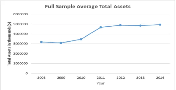
Figure 2 Full sample Average Total Assets ... 29

Figure 3 Full sample Average Total Liability ... 29

Figure 4 Average Debt to Equity by Sector ... 30

Figure 5 Average Debt to Asset by Sector ... 31

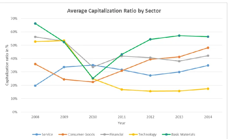
Figure 6 Average Capitalization Ratio by Sector ... 32

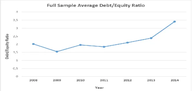
Figure 7 Full Sample Average Debt to Equity Ratio ... 34

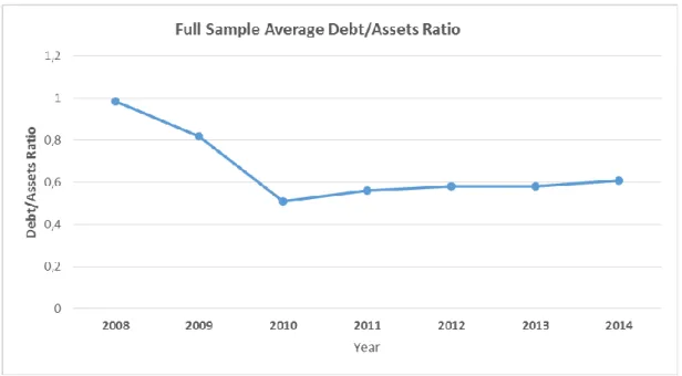
Figure 8 Full Sample Average Debt to Asset Ratio ... 35

Figure 9 Full Sample Average Capitalization Ratio ... 37

Tables

Table 1.2 Test Statistic on Debt to Equity ... 35

Table 2.1 Positive & Negative Ranks on Debt to Asset ... 36

Table 2.2 Test Statistic on Debt to Asset ... 36

Table 3.1 Positive & Negative Ranks on Capitalization ... 38

Table 3.2 Test Statistic on Capitalization ... 38

Table 4.1 Capital Structure change 2008 ... 39

Table 4.2 Capital Structure change 2014 ... 39

Equations

Equation 1.2 Modigliani & Miller proposition II ...9

Equation 1.3 Modigliani & Miller proposition I: with tax ... 10

Equation 1.4 Modigliani & Miller proposition II: with tax ... 10

Equation 1.5 Weighted Average Cost of Capital: with tax ... 10

Equation 1.6 Debt to Equity ratio... 19

Equation 1.7 Debt to Asset ratio ... 19

Equation 1.8 Capitalization ratio ... 20

Equation 1.9 Difference between two populations ... 22

Equation 1.10 Wilcoxon Signed-Rank Test T-value ... 23

Equation 1.11 Mean of T-value ... 23

Equation 1.12 Standard deviation of T-value ... 23

Equation 1.13 Standardized z-value ... 23

Appendices

Appendix 2 Annual Company Debt to Equity Ratio ... 50

Appendix 3 Annual Average Sector Debt to Equity Ratio ... 50

Appendix 4 Annual Company Debt to Asset Ratio ... 51

Appendix 5 Annual Average Sector Debt to Asset Ratio ... 51

Appendix 6 Annual Company Capitalization Ratio ... 52

Appendix 7 Annual Average Sector Capitalization Ratio ... 52

Appendix 8 Descriptive Statistic on Debt to Equity Ratio ... 53

Appendix 9 Descriptive Statistic on Debt to Asset Ratio ... 53

Appendix 10 Descriptive Statistic on Capitalization Ratio ... 53

1

Introduction

1.1

Background

1.1.1 Initial Public Offering (IPO)

Draho (2004) defines an Initial Public Offering (IPO) as when a company decides to sell its shares for the first time to public investors and consequently in the stock market. According to Jenkinson & Ljungqvist (2001) a firm has the opportunity to generate new equity for investors or they already possess privately-owned existing equity. Usually, a combination of both options are applied by organizations.

In the late 1990s, IPO’s received massive attention for successively creating new businesses, job opportunities and positive investment returns. However, with time, investment banks showed their true colorsand left the public with a negative view of IPO’s. Most people agree with the fact that IPO’s are rather complicated to understand. Relying on inadequate data and a misinterpretation of the IPO process, the public is held clueless and thus forced to draw incomplete conclusions regarding why firms choose to go public in the first place and how an IPO functions (Draho, 2004).

One of the major advantages of going public is to acquire capital, in order for the company to grow further (Ritter & Welch, 2002). Obviously, receiving capital from banks is one way to proceed, however, according to Rajan (1992) it is significant for a company to not be dependent on one source of income. Raising capital from various sources could decrease credit and debt, and thus lead to investment possibilities. Additionally, offering shares to the public will hopefully lead to publicity and thus increase the probability of attracting new investors to the company (Ritter & Welch, 2002).

In outdated course books it is mentioned that the primary reason for going public is to lower the cost of capital and the pecking order of financing. However, according to Brau & Fawcett (2006) the main motivation for firms to embark on an IPO is to offer shares to the public for purchase.

Going from a private firm to a publicly-traded company comes with several and substantial changes. For instance, since the company is no longer private it cannot withhold information from the public which was possible before. The firm’s financial performances and processes need to be reported and explained if they deviate from the planned budget. Legal issues need to be considered, the economic structure needs change, and a greater responsibility is put on

management teams since they now need to consider diversified stakeholders. Additionally, when a firm decides to go public, the company itself is seen as a threat and is thus vulnerable to a more competitive market (Draho, 2004).

As mentioned previously, the IPO process is complicated to say the least. Initially, a firm employs an investment bank (underwriter), which takes charge of the entire process and then proceeds with an extensive evaluation of the firm (due diligence), values shares and acts as a helping guide along the process. Furthermore, after the estimation of the firm the investment bank will enclose valuable information regarding the financial standing and growth predic-tions. This is called a prospectus and is used by prospective shareholders to attain infor-mation regarding the firm before deciding whether or not to purchase shares in the IPO. After the publication of the prospectus, the investment bank aims to market the firm to the public by contacting probable stakeholders and by arranging road show meetings, with the purpose of promoting the firm and its shares. During this time period potential investors are able to acknowledge the investment bank if there exists an interest before the company is listed on the stock exchange, this is also known as a subscription period. When the subscrip-tion period has ended, the investment bank acknowledges the interested investors with a proposal regarding the allocation of shares among the shareholders. Eventually, the first shares are traded on the stock exchange for the first time after the investment bank and the issuing firm have decided upon the allocation of shares (Jenkinson & Ljungqvist, 2001).

1.1.2 Capital Structure

In order for a firm to prosper and succeed in today’s market, investments in various types of sectors such as employment of staff, buildings and equipment are vital. Due to this, various types of credit are needed (Chorafas, 2005). Depending on the size of the company, a firm can increase its money supply by obtaining credit in public debt markets or be financed by local banks, which is often the case for most small firms (Berger & Udell, 1995).

Furthermore, Ross, Westerfield, & Jaffe (2002), argued that a firm’s capital structure is what determines the true value of a firm. Capital structure is the combination of debt and equity which a firm uses in order to support and maintain its continuing operations and develop-ment. Since the capital structure affects the value of a firm, it is in the best interest of a firm to measure the ratio of debt to equity, in order to capitalize on firm value. By increasing the market value the firm also capitalizes on shareholders wealth. According to McMenamin (1999), debt and equity is not as easy to comprehend as it may seem. They come in various

forms, such as, preferred stocks, common stock, retained earnings, bank credits, bonds, line of credit and accounts payable.

Corporations who have large amounts of equity can to a greater extent withstand from bank-ruptcy, since shares are not required to be submitted to stakeholders during such circum-stances (Finnerty & Emery, 2001). On the other hand, companies which have been financed by debt are obligated to pay interest on the debt received, despite positive or negative results (Kamsvåg, 2001). This means that when a recession occurs it will come with greater risk for a company with equivalently much debt. In contrast, during economic growth, a company with equivalently much debt will be more lucrative than a company with equally much in equity (Pike & Neale, 1993)

There exists numerous theories regarding the optimal capital structure in a firm and whether or not it is an appropriate measurement tool for firm value. If there does exist an optimal capital structure, it is the one that makes the most of investors capital. Several theories such as trade-off theory, pecking order theory and Modigliani and Miller’s irrelevance theory at-tempts to reason if this statement is true or false (Myers S. C., 2001). However, a further explanation regarding these capital structure theories will be presented in the theoretical framework section.

1.2

Problem Discussion

Managing a firm’s capital and obtaining the most optimal capital structure is a complex ques-tion to answer. Dealing with this type of issue is of great importance since management of capital is the key factor to consider when opening or expanding a business (Pike & Neale, 1993).

Furthermore, the process of a firm conducting an initial public offering is complex to say the least and therefore one needs to consider various factors before making this decision. Alt-hough there have been plenty of studies in the field of IPOs and capital structures separately, there have not been many investigations regarding the effect on capital structure before and after an initial public offering. However, some research within this area of study has been conducted and will be discussed in the following section.

Several individuals have attempted to present an optimal capital structure model for firms but have failed to do so. At the moment there does not exist an ideal capital structure theory that is suitable for all and there is no reason to expect one in this thesis or in the near future either (Matthews, Vasudevan, Barton, & Apana, 1994; Barton & Matthews, 1989).

However, Myers & Majluf (1984) aimed to solve this issue with his pecking order theory, where he argued that organizations attempt to finance their firm by initially using the profits from preceding years. If this is not sufficient the firm will take a loan from the bank and finally issue new shares. Managing a firm does not always go according to plan, which often implies the need to fund the business in different ways than intended in beforehand. For example, in the case of increasing growth and demand, firms borrow money from banks and thus increase their debt, instead of issuing equity, when the firm’s internal liquidity is not able to cover the expenses. However, the decision to finance a firm’s capital by debt or equity comes with business and financial risks. If a company decides to finance their capital with too much debt the risk of bankruptcy increases (Carter, Van Auken, & Carter, 2006). The issue of risk is a strategic dilemma in itself and deviates depending on the business and the executive’s assumption of how much risk the firm can endure (Barton & Matthews, 1989). Modigliani & Miller (1958), discuss the advantages of certain mixtures of debt. They argue that financing does not matter. They proved that firm value, cost of capital and availability of capital is not dependent on the choice of debt and equity financing. They presumed that capital markets are seamless and flawless wherein monetary improvement would eliminate any abnormality from anticipated equilibrium. Although, if one considers taxes, information differences and agency costs, financing seem to matter after all. By taking these aspects into deliberation, capital structure theories tend to differ. The tradeoff theory highlights taxes, free cash flow theory underscores agency costs and pecking order theory underlines differ-ences in information (Myers & Majluf, 1984).

When investigating previous research on initial public offerings a common occurrence is the concept of underpricing, agency theory and hot issue markets. Although, these concepts are not the sole purpose of the thesis, a brief explanation is needed to comprehend the initial public offering process.

Underpricing is a capital loss which occurs when the closing price is higher than the offering price after the first day the shares have been offered to the public (Jenkinson & Ljungqvist, 2001).

Agency theory or relationships occur when an individual (principal) has the authority to del-egate decision making on another individual (agent) (Jensen & Meckling, 1976).

The study of ‘’hot issue markets’’ reflects on the positive opportunities of emerging into an IPO because of an increasing demand of a special product or service (Ritter, 1984). This theory of taking advantage of an increasing demand could be linked to bullish stock markets - an optimistic market where prices are rising or are expected to rise.

Since the authors of this thesis have decided to investigate if there is a difference in the capital structure pre and post an initial public offering, the main focal point will lie on capital struc-ture and briefly discuss initial public offerings. However, this research will not investigate further into the complex issue of finding an optimal capital structure and whether underpric-ing is eminent in the financial market, since these areas have been studied comprehensively in the past decades.

1.3

Purpose

The focus of this study is to examine the capital structure in firms before and after an Initial Public Offering. We will focus on the following ratios when evaluating the capital structure:

 Debt to equity ratio

 Debt to asset ratio

 Capitalization ratio

By examining these ratios we will try to detect the possible differences in values of these ratios before and after an IPO and if there are any trends in certain industries. The sample is based on 31 American companies that were listed on the New York Stock Exchange (NYSE) in 2010. The aim is to observe how the capital structure changes between 2008 and 2014.

1.4

Delimitations

Previous studies on capital structure have intended to explore whether or not an optimal capital structure exists. However, since this area is a complex ongoing debate, it has been decided to not investigate this issue further. Instead, the focus is to examine whether or not an IPO has an effect on capital structure.

The data set has been collected from the New York Stock Exchange (NYSE) on companies which performed an Initial Public Offering in 2010. There are numerous companies who went public during this time period and thus it may come as a surprise that the sample size only consists of 31 companies. The reason for this is that companies which presented their annual reports in figures other than USD were excluded, since it would be too time consum-ing to change all values. Furthermore, several companies did not express certain values i.e. Short-term debt and long-term debt, and therefore they were excluded as well.

Moreover, there was an issue with the debt to equity ratio and whether or not to divide total liabilities with shareholder’s equity or sum up short-term debt with long-term debt and then divide it with shareholder’s equity. Since there does not exist an optimal debt to equity for-mula and there were difficulties with attaining short-term debt from the company’s annual reports it was decided to use total liabilities divided by shareholder’s equity as the formula for debt to equity ratio. This may have had an impact on the debt to equity ratios.

Also, when investigating changes on a certain issue, a long time period is recommended to be able to notice any significant differences. The authors could have investigated previous years such as 2006 and 2007, however, since it was difficult to find annual reports for those years and a lot of important financial values were missing, 2008 was set as the starting point for the sample size.

The reason why certain sectors were chosen and some are not is because some sectors only consisted of one or two companies and thus they were excluded.

Additionally, since the timespan was set to 2008-2014, an important restriction to take into consideration is the financial crisis which occurred in 2008 and 2009. Although, the financial crisis was not mentioned or analyzed in detail it may have had an effect on the final results and conclusion respectively.

2

Theoretical Framework

2.1

Methods of Financing

To clarify the definition of the term debt one might simply say that it is the process of bor-rowing money with the promise to repay the amount borrowed, the principal, as well as the interest on the principal. There are various types of debt financing, such as selling bonds, bills, or notes to plain individuals or investors, individual or institutional (Creamer, Dobrovolsky, & Borenstein, 1960).

2.1.2 Equity Financing

The other method for an entity to finance its operations is the act of equity financing. It refers to the procedure of obtaining capital by selling shares of the company. The individual, or institution who buys the share, the shareholder, receives a specified amount of ownership in the company. In the financial world, equity financing is often associated with larger public companies trading stocks on the various stock exchanges. In contrast, equity financing is a part of the capital structure in privately held companies as well. However, due to the features of a private firm, the possibility to sell shares is rather limited (Creamer, Dobrovolsky, & Borenstein, 1960).

2.2

Capital Structure

2.2.1 Modigliani and Miller Theorem

In the following section an analysis and review of Modigliani & Miller’s proposition I and proposition II with and without the impact of taxes is outlined.

Proposition I: The value of a firm is the same independent of the fraction of debt or equity

in the capital structure (Modigliani & Miller, 1958).

Proposition II: The cost of equity increases with the percentage of debt in the capital

struc-ture (Modigliani & Miller, 1958).

2.2.1.1 Modigliani & Miller Proposition 1: No taxes

Franco Modigliani and Merton Miller performed an extensive research in the area of capital structure in 1958. The study resulted in the Modigliani and Miller theory, even called the irrelevance theory. The theory states that the value of a firm is constant and non-changing regardless of which form of capital structure a company chooses. In other words, the value of the firm is not affected by the amount of leverage a firm has. In order for the stated argument to hold, some assumptions were made (Modigliani & Miller, 1958).

 No existence of transaction costs

 Individuals and corporations borrow at the same rate

 There are no costs to bankruptcy

 No existence of personal or corporate tax

 Perpetual cash flows

 All agents are rational

Moreover, when these assumptions are satisfied, the following equation holds: 𝑽L = 𝑽U

𝑽𝑳= The value of a levered firm

𝑽_𝑼=The value of an unlevered firm

Equation (1.1), Modigliani & Miller proposition I (1.1)

As one can conclude from the equation, the value of a levered firm is the same as the value of an unlevered firm (Modigliani & Miller, 1958). This statement defines proposition I made by Modigliani and Miller and can directly be related to the act of homemade leverage. Home-made leverage is explained as the procedure of individuals borrowing on the same terms as a firm in order to create an impact on the leverage of the firm.

2.2.1.2 Modigliani Proposition II: No taxes

As earlier stated in this section of the study, the second proposition, based on specific as-sumptions, states that the cost of equity of a firm increases linearly with the percentage of debt to equity.

The second proposition has its foundation in the following equation:

𝒓

= 𝒓

+ (𝒓

+ 𝒓

) 𝑩 𝑺

⁄

Equation (1.2), Modigliani & Miller proposition II (1.2)

The obtained equation above is derived from a rearrangement of the Weighted Average Cost of Capital (WACC) formula. Evidently, as indicated in the restructured formula above, the cost of equity is in a positive linear relationship with the level of leverage in a firm. Since, the return on asset (

r

r

Moreover, according to proposition I, a firm’s WACC is not affected by the capital structure of the firm. In order to supply the necessary conclusion, volatility has to be included in the analysis of the propositions. When a firm intentionally increases the level of leverage, the level of risk increases as well. Firms with a levered structure tend to have a smaller amount of the operating income divided on the outstanding shares. The return on equity might show a higher value, however, the risk increases as well (Modigliani & Miller, 1958).

2.2.1.3 Modigliani and Miller Proposition I: With Taxes

In the list of assumptions provided above, one of these assumptions, namely the one stating that there are no taxes for individuals nor corporations has been a subject of criticism when dealing with the Modigliani and Miller theory. The reason is obvious, the assumption is highly unrealistic and difficult to accept since every company and individual has the obligation to pay taxes on their income.

However, a levered company can experience a reduction in tax expenses by a phenomenon called ‘’tax shield’’. With the help of tax shields, companies with a high leverage have the ability to pay a smaller amount of tax than an all equity firm.

Thus, to explain it algebraically, the value of a levered firm is equal to the value of an un-levered firm with the added present value of the tax shield given by the debt. Corporate tax is illustrated as Tc.

𝐕_𝐋 = 𝐕_𝐔+ 𝐓_𝐂

Equation (1.3), Modigliani & Miller proposition I: with tax (1.3)

With the added risk-free debt and tax, the company has the capacity to in a sense optimize its market value (Modigliani & Miller, 1963).

2.2.1.4 Modigliani and Miller Proposition II: With Taxes

Earlier it was stated that proposition II by Modigliani and Miller showed a clear positive linear relationship between the cost of equity and the percentage of debt in the capital struc-ture. The same conclusion holds even if we take the impact of taxes in mind as seen in the equation below:

𝒓

= 𝒓

+ (𝒓

+ 𝒓

) × (𝟏 − 𝑻

) × 𝑩 𝑺

⁄

With taxes now being included in the formula, the new design of the WACC is seen below: 𝑾𝑨𝑪𝑪 =_𝑫+𝑬𝑫 × 𝒓_𝒅× (𝟏 − 𝑻_𝒄) +_𝑬+𝑫𝑬 × 𝒓_𝒆

With corporate tax included, the value of WACC decreases with a higher level of leverage in a firm. Thus, assuming that corporate taxes exist, the value of the firm will increase alongside with the level of leverage in a firm due to the decrease in the WACC (Modigliani & Miller, 1963).

2.2.2 Trade-Off Theory

The trade-off theory concerns the capital structure in an important manner. The theory eval-uates the marginal costs of debt and equity and tries to conclude the optimal amount of debt, which is reached at the trade-off point. According to the theory of Modigliani & Miller (1963), firms should be highly leveraged in order to benefit from the tax shield. On the other hand, the theory did not take the bankruptcy costs in mind, which occur in the real world. In order to determine the optimal level of debt, one must examine the most important de-terminants of a firm’s level of debt, namely agency costs and financial distress.

2.2.2.1 Agency Costs

The first type of agency cost concerns the difficulties and problems regarding the difference in interests between the managerial sector and the shareholders, explicitly, the agency cost of equity. Moreover, it also covers the challenges of information between management and shareholders, principal and agent respectively. Conflicts between managers and shareholders can occur during periods of uneven distribution of wealth, which is related to the activities of the managers. Thus, the efficiency of managerial activities drives the relationship between the principal and the agent and determines how well the association is between them (Jensen & Meckling, 1976).

Under specific circumstances, when a firm is under the pressure of liquidation, managers always want to continue the firm’s operation even though debt holders consider bankruptcy. However, firms in these situations can avoid these kind of problems by providing the inves-tors the ability to carry out a liquidation if the firm’s cash flows do not reach a desirable level. Increasing levels of debt increases also the risks of default, which is positive for the investors, On the other hand, this outcome demands higher evaluation costs related with the liquidation (Harris & Raviv, 1991).

A second important part of agency costs is the agency cost of debt. Such costs occur when there is a conflict between stockholders and debtholders. Alongside with a firm´s increasing level of debt in the capital structure, bondholders take part of risks related to various actions

driven by the managers. As the manager and shareholders control the firm’s future invest-ment strategies, they can choose a variety of strategies to benefit them. On the other hand, the bondholders, who provide the capital, are victims of the risk and can only recognize the costs of these actions.

There are four different situations in which agency cost of debt can arise. These situations occur when investors undertake risky projects, when investors undertake negative net pre-sent value (NPV) projects, milking property situation and incentives toward underinvestment (Megginson, 1997).

2.2.2.2 Financial Distress

According to the theory of Modigliani & Miller (1963) a highly leveraged firm is provided tax benefit. However, since companies are obligated to conduct interest and principal pay-ments, it puts a pressure on the firm. The worst scenario of financial distress is the issue of bankruptcy. A firm approaching a state of bankruptcy faces a variety of difficulties ranging from lack in moral from the employees to difficulties in managing the financial operations. Moreover, if a firm faces a state of liquidation, the ownership of the assets have the right to be legally transferred from the stockholder to the bondholders. When dealing with bank-ruptcy costs, one might refer to two parts of these costs, namely direct and indirect costs (Haugen & Senbet, 1988).

Direct costs are related to lawyers and accountants fees as well as other professional’s fees. Moreover, direct costs also include the value of managers administrating in the procedure of a bankruptcy. Furthermore, the impact of a bankruptcy depends partly on the size of the firm. It was stated by Warner (1977), that direct costs tend to decrease when the size of a firm increases.

Indirect costs include the lost values of possible sales and profits and therefore they are not losses of economic activities itself. Additionally, these costs also deal with the incapability of the firm to issue securities or increase credit (Warner, 1977).

Edward Altman conducted a study in 1984 where he gathered a sample of 19 firms, which all went bankrupt between the years of 1970 and 1978. In his investigation he compared expected profits with actual profits and concluded that the value of arithmetic indirect bank-ruptcy costs to be 10, 5% of firm value. It was also identified that the sum of both direct and indirect costs together added up to more than 20% of firm value (Altman, 1968).

The mentioned investigations and conclusions gives one enough evidence to believe that the costs of bankruptcy are sufficiently large to support the trade-off theory of optimal capital structure.

2.2.3 Pecking-Order Theory

Comparing the trade-off theory to the pecking order theory, one might discover a few dif-ferences. According to the pecking order theory firms prefer internal to external financing, as well as debt to equity if it is to issue securities. Moreover, in the original pure pecking order theory, a firm cannot in advance define a debt to value ratio (Myers S. C., 1984). Myers (1984) defined the theory by lining up the following preferences:

1) Firms prefer internal finance

2) The firms adjust their dividend to their investment opportunities.

3) Sticky policies regarding dividends as well as changes in profitability and investment opportunities lead to a scenario where the internally generated cash flow may be higher or lower than investments.

4) In the scenario where external finance is essential, firms start with debt, then possibly hybrid securities such as convertible bonds. At last they choose equity as a least fa-vorable option.

2.3

IPO Theories

Underpricing is a phenomenon related to IPOs and refers to the situation when the offering price is lower than the market price on the first trading day and thus the stock is underpriced. This could be recognized by the stocks a short period after issuance. The initial returns tend to be higher and the stocks gain value at a remarkable speed. One significantly investigated reason for this kind of phenomenon is called ‘’the winner’s curse’’, which deals with the importance and features of information.

Kevin Rock (1986) refined his model regarding the value of information for investors, which he introduced in his PhD dissertation (1982). Moreover, Rock (1986) explains further the model where investors can choose to inform themselves and thus value shares corresponding to their accurate value. However, information of this kind is costly and therefore a segrega-tion is developed between two groups, informed and uninformed investors. Informed inves-tors will solely purchase underpriced stocks while uninformed invesinves-tors tend to buy all issues. Hence, the uninformed investors will receive the majority of the overpriced stocks and a minority of the underpriced stocks. (Rock, 1986)

Furthermore, firms facing large levels of uncertainty regarding their value will benefit of us-ing the ‘’best-efforts method’’, where underwriters attempt to sell as much as possible of the shares to the public. Thus, the issue of less adverse selection decreases since unsubscribed offers become withdrawn (Rock, 1986; Beatty and Ritter, 1986).

2.3.2 Hot Issue Markets

In the field of finance the concept hot issue markets has been debated and investigated thor-oughly in the last decades. Ibbotson & Jaffe (1975), were the first to introduce the concept of hot issue markets. According to Helwege & Liang (2004), the financial market can expe-rience a hot and cold issue market. Hot issue markets are defined as bull markets where underpricing, oversubscription and offerings are high. On the contrary, cold markets have been categorized with bear markets in which oversubscription, amount of underpricing and issuing volume are low.

Hot issue markets occurs when stock issues have experienced a significant increase from their original offering prices and are higher than the average. It is a time span in which initial

returns are unusually higher than normal. In an investigation Ibbotson & Jaffe (1975) in-spected the serial dependency of new issues between two months and found that hot issue markets can be predicted for the upcoming month if the market in the current month is hot. However, since the series is static it implies that one day it will evaporate. This means that investors could try to avoid investing during cold market issues and instead invest profoundly in hot issue markets which has been anticipated. However, predicting markets is not practical since new offerings are limited, regulated and oversubscribed. Moreover, predicting hot issue markets would imply that demand for stocks would exceed supply of stocks significantly and thus abolish the opportunity of receiving profit. However, firms could attain higher prices by simply issuing after months of low initial returns and exploit historic data figures to time an offer (Ibbotson & Jaffe, 1975).

Ritter (1984), attempted to prove the presence of hot issue markets in the finance market with the help of the winners curse model which was introduced by Rock (1986). Ritter was able to find a correlation among high initial returns and volume, which Ibbotson (1975) was not able to. He argued that after high stock market returns (hot issues), IPO volumes are high while average initial return is low. The initial return is low because of inferior issue time, which indicates low demand or high offering prices where price determination has been mis-judged.

More modern theories have come to the conclusion that during hot issue markets, companies usually are affected by a bandwagon effect. For example, if a business within a particular industry decides to go public and does so successfully, more companies from the similar industry will undertake an initial public offering, simply because the first company has been prosperous (Benvenistea, Busabab, & Wilhelm, 2002).

2.4

Risk

Two fundamentals of risk are considered to be important factors in the decision of capital structure, namely the business risk and the financial risk of the firm. These types of risks will thus be discussed in the following section.

2.4.1 Business Risk

Business risk refers to the possibility of experiencing lower profits than anticipated, or even experiencing a loss in profits. There are various factors determining a firm’s level of business risk, factors that appear more or less depending on which industry the company is active in. These factors are:

1. The irregularity of sales volume beyond the business cycle. When firms

expe-rience heavy fluctuations in their sales volume above the business cycle, they are ex-posed to a greater amount of business risk.

2. The irregularity of selling prices. There are industries where prices remain stable

year after year without any major variations and companies succeed in increase prices over some period. Although this is true for the majority of consumer products, other industries experience instability in selling prices. Such industries, where competitive pricing is common, business risk tends to be higher.

3. The irregularity of costs. Since effective production is essential for successful

com-panies, an increased changeability in costs for a firm producing its output leads to a higher business risk.

4. Impact of market power. Firms that have a great deal of market power have the

capacity to control their current costs and the price of their outputs. In contrast, firms that are active in a competitive market environment do not have the same priv-ilege. Hence, firms experiencing greater market power also experience less business risk.

5. The effect of product diversification. When a firm has a well-diversified set of

products it experiences a less fluctuating level of operating income. Thus, a firm hav-ing a stable operathav-ing income without any major variations experiences a minimized business risk.

6. The impact of the level and rate of growth. The effect of a higher growth on a

company is mostly positive, however there are some factors leading to a higher busi-ness risk. A firm experiencing a rapid growth does not solely experience a fluctuation in operating income because of higher demand for its products or services. It also

undergoes major internal operational changes all contributing to a high variety in operational income and thus an increased amount of business risk.

7. The degree of operating leverage. Operating leverage has a great deal with the use

of assets having fixed costs. Since, this relation is evident, high levels of operating leverage in a firm leads to a more sensitive earnings before interest and tax (EBIT). Therefore, the amount of operating leverage in a sense decides the level of business risk in a firm (Moyer, McGuigan, & Kretlow, 2000).

2.4.2 Financial Risk

The second fundamental of risk concerning capital structure is the financial risk. Financial risk refers to the additional variations in the level of earning per share (EPS) and the increased probability of meeting contractual financial obligations when a firm uses fixed-cost sources of funds. When a firm uses an increased amount of debt and preferred stocks, the financial costs increase alongside with an increased EBIT, and thus the company can continue to operate its activities. Being able to increase returns to shareholders is in the deepest interest of the firm and that is why the use of fixed-cost financing is widespread. Moreover, the financial risk can be directly related to the possibility that equity holders will lose money when they invest in a leveraged company (Moyer, McGuigan, & Kretlow, 2000).

3

Method

3.1

Methodology

3.1.1 Quantitative Research Methodology

Håkansson (2013), argued that a researcher must choose between a qualitative (non-numer-ical, quantitative (numerical) or a mix of both research methods. One of the three alternatives must be chosen since it has an impact on the entire research project.

One of the major advantages with the quantitative method is that it enables the researcher to acquaint with the problem or concept of interest. Firstly, the results need to be computed and summarized using numerical data. Secondly, some sort of mathematical procedure needs to be applied to analyze the numerical data. Finally, the end result needs to be presented with statistical terms and expressions (Charles, 1995).

3.1.2 Philosophical Assumptions

A philosophical assumption or paradigm is a significant part of a research since it guides the whole research process. There are numerous assumptions to choose from depending if one chooses to implement the quantitative or qualitative research method. For instance, positiv-ism, realpositiv-ism, interpretevism and criticalism are all philosophical paradigms.

The positivist paradigm supports the quantitative research method and argues that the world is observable and measurable (Glesne & Peshkin, 1992). The principal belief of a positivist is that any study, whether it is on consumers or marketing phenomena should be scientific. The positivist paradigm promotes quantitative methods by measuring theories, hypothesis and phenomena in an objective and scientific manner and therefore it was chosen for this study (Malhotra & Birks, 2007).

3.1.3 Research Approaches

The aim of a research approach is to draw suppositions and prove or disprove hypotheses. The inductive approach is used in qualitative methods while the deductive method is em-ployed in quantitative methods and thus, the abductive approach is a mix between quantita-tive and qualitaquantita-tive methods. Since this is a quantitaquantita-tive method the authors have decided to implement the deductive approach (Håkansson, 2013). Someone who follows a positivism approach aims to authenticate his or her research with deduction (Malhotra & Birks, 2007). The deductive approach examines existing hypotheses and theories and intends to prove or disprove them with the help of statistical calculations. The hypothesis must be functioning,

computable and mention which variables will be applied, how they will be measured and what the estimated conclusion will be (Håkansson, 2013).

3.2

Financial Ratios

The following financial ratios have been chosen to measure the capital structure of each company. These ratios will then be analyzed using a statistical test in order to prove or dis-prove the predetermined hypothesis and thus the research question.

3.2.1.1 Debt to Equity Ratio

The debt to equity ratio is a leverage ratio that examines the relationship between a com-pany’s total liabilities to its total shareholder equity. The ratio expresses what fraction of debt and equity the company is using in order to finance its assets (Berk & DeMarzo, 2011). The formula for the debt to equity ratio is seen below:

Debt to equity ratio = 𝑻𝒐𝒕𝒂𝒍 𝑳𝒊𝒂𝒃𝒊𝒍𝒊𝒕𝒊𝒆𝒔 𝑺𝒉𝒂𝒓𝒆𝒉𝒐𝒍𝒅𝒆𝒓𝒔 𝑬𝒒𝒖𝒊𝒕𝒚

Equation (1.6), Debt to Equity ratio (1.6) 3.2.1.2 Debt to Asset Ratio

The debt to asset ratio indicates the proportion of a company’s assets which are financed through debt. In the case of the ratio being less than 1, it indicates that a significant propor-tion of the assets are financed by equity. In contrast, if the ratio is higher than 1, it indicates that the assets are mostly financed through debt. The debt to asset ratio is often used to determine the financial risk of a company, which you can read about in the section of ‘’risk’’ (Berk & DeMarzo, 2011).

The ratio is calculated by dividing total liabilities by total assets as seen below:

Debt to asset ratio = 𝑻𝒐𝒕𝒂𝒍 𝑳𝒊𝒂𝒃𝒊𝒍𝒊𝒕𝒊𝒆𝒔 𝑻𝒐𝒕𝒂𝒍 𝑨𝒔𝒔𝒆𝒕𝒔

3.2.1.3 Capitalization Ratio

The capitalization ratio is a measurement of the amount of debt related to the capital struc-ture or capitalization. The ratio provides important information about the company’s capital structure and the use of leverage (Berk & DeMarzo, 2011).

The capitalization ratio is calculated by dividing long term debt by the sum of long term debt and shareholders’ equity as seen below:

Capitalization Ratio = 𝑳𝒐𝒏𝒈 − 𝒕𝒆𝒓𝒎 𝒅𝒆𝒃𝒕

𝑳𝒐𝒏𝒈 − 𝒕𝒆𝒓𝒎 𝒅𝒆𝒃𝒕 + 𝑺𝒉𝒂𝒓𝒆𝒉𝒐𝒍𝒅𝒆𝒓𝒔′_{𝑬𝒒𝒖𝒊𝒕𝒚}

Equation (1.8), Capitalization ratio (1.8)

3.3

Data Collection

Secondary data is information that has been retrieved for another purpose than the problem at hand. For instance, articles, books, information etc. made available by governments, busi-nesses and databases are all classified as secondary data. The benefit with secondary sources is cost and time efficiency. Analyzing secondary data before conducting the actual primary data is recommended. The disadvantages with secondary data is how valid and reliable the data is to the specific research question, since it has been collected for another purpose in beforehand (Malhotra & Birks, 2007).

Primary data, on the other hand, is when data is collected to answer the research question at hand. It is not something that has been conducted previously or by someone else. It is sig-nificant to note that primary data should not be composed until the secondary data has been entirely analyzed. Compared to secondary data, conducting primary data is both expensive and time-consuming. Primary data is tailored since it helps to answer a specific research question or market phenomena and thus cost huge amounts of money for organizations to conduct (Malhotra & Birks, 2007).

The New York Stock Exchange (NYSE) was used to find companies which performed an IPO in 2010. Once a satisfied number of companies in our sample was collected, Yahoo finance was applied to find and distribute each firm according to their respective sectors. In order to find the financial values the authors simply entered each company’s website to find the annual reports. Since the aim is to examine whether or not the capital structure is affected before or after an IPO, annual reports were gathered from 2008-2014. This in order to see a difference before the IPO and a few years after the IPO.

Once all companies and financial values were retrieved from the annual reports they were put in a database using Microsoft Excel. The graphs presented in the result section have been calculated and completed using Microsoft Excel. Once all financial ratios and graphs were implemented, a statistical test was performed in order to prove or disprove our hypothesis. This was possible using the Statistical Package for the Social Sciences (SPSS).

3.4

Data Analysis

After conducting the financial ratios and completing the graphs and figures the aim was to analyze these results with the help of statistical methods. Statistical methods can be divided into two major categories, namely, descriptive and inferential statistics. Before explaining what these are, one needs to understand the meaning of a population and sample. A popu-lation is the total amount of individuals or objects that is under investigation. A sample is basically a subset of the actual population being analyzed (Allua & Thompson, 2009). For instance gender, age and nationality could all be samples from the entire population. Descriptive statistics aim to analyze and describe a sample of interest. However, with infer-ential statistics the purpose is to analyze the chosen sample data and then make predictions or generalization about the population. This is often done to save time and money for re-searchers (Allua & Thompson, 2009). In this thesis the inferential statistics method has been chosen because the sample data of interest will represent and provide proof to the entire population on whether or not capital structure is affected by an IPO.

However, choosing the correct statistical test is difficult to say the least. There are numerous tests to choose from and each is dependent on what one wants to measure and observe. After deciding on applying inferential statistics, the next question was to choose a parametric or non-parametric test since a combination of both is not acceptable. A parametric test is used when the results show a normal distribution. If one is unsure whether or not the results are normally distributed or not, the non-parametric method should be used. Since that is the case, the non-parametric method is applied (Marshall & Jonker, 2011).

The Wilcoxon Signed-Rank test is an inferential, non-parametric statistical test which com-pares the difference in median value from two populations. A sign-test is similar to the Wil-coxon Signed-Rank test but differs since it not only analyzes signs but also degrees of differ-ences between paired values. This is completed by taking into account both the positive and negative ranks (Aczel & Sounderpandian, 2008).

In Wilcoxon’s Signed-Rank test, the null hypothesis states that the median difference be-tween two populations is equal to zero. The alternative hypothesis states that the median difference between the same two populations is not equal to zero and can be seen below:

𝐻𝑂: 𝑇ℎ𝑒 𝑚𝑒𝑑𝑖𝑎𝑛 𝑑𝑖𝑓𝑓𝑒𝑟𝑒𝑛𝑐𝑒 𝑏𝑒𝑡𝑤𝑒𝑒𝑛 𝑡𝑤𝑜 𝑝𝑜𝑝𝑢𝑙𝑎𝑡𝑖𝑜𝑛𝑠 𝑖𝑠 𝑒𝑞𝑢𝑎𝑙 𝑡𝑜 𝑧𝑒𝑟𝑜

𝐻_𝐴: 𝑇ℎ𝑒 𝑚𝑒𝑑𝑖𝑎𝑛 𝑑𝑖𝑓𝑓𝑒𝑟𝑒𝑛𝑐𝑒 𝑏𝑒𝑡𝑤𝑒𝑒𝑛 𝑡𝑤𝑜 𝑝𝑜𝑝𝑢𝑙𝑎𝑡𝑖𝑜𝑛𝑠 𝑖𝑠 𝑛𝑜𝑡 𝑒𝑞𝑢𝑎𝑙 𝑡𝑜 𝑧𝑒𝑟𝑜 Initially, one lists the pairs of observations on two variables, in our case, comparing two years from one of the financial ratios. After this, the differences are calculated for every pair and finally the total values of the differences in D are ranked, as seen below:

𝐷 = 𝑋1− 𝑋2

Equation (1.9), Difference between two populations (1.9)

Since the aim is to investigate whether capital structure is affected by an IPO or not, the following hypothesis will be used and analyzed. The capital M stands for the median and the D stands for the difference between two variables or populations (Aczel & Sounderpandian, 2008).

𝐻₀: 𝑀_𝐷 = 0 𝐻_𝐴: 𝑀_𝐷 ≠ 0

In this thesis, the statistical test will be applied to the debt to equity ratio, debt to asset ratio and capitalization ratio and investigate the year of 2008 and 2014 to compare if there exists any difference in the median values or not. These years were selected since 2008 is two years prior to the IPO and 2014 presents the latest values that the authors were able to retrieve from the company’s annual reports.

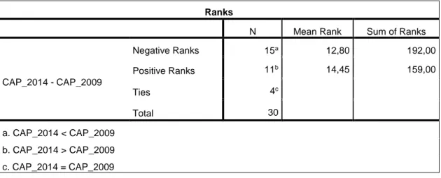
For instance, when investigating debt to equity ratio, the Wilcoxon signed rank test first calculates the difference between two pairs, and then sums up the positive and negative ranks. The T is extracted by selecting the smaller sum value of either the negative or positive ranks. ∑ (+) is the sum of the ranks of the positive differences and ∑ (-) for the negative differences. For instance if the positive rank is 70 and the negative rank is 50, the T-value will be 50 since it is the lowest sum of the two values (Aczel & Sounderpandian, 2008).

𝑇 = min[ ∑ (+), ∑ (−)]

Equation (1.10), Wilcoxon Signed-Rank Test T-value (1.10)

Moreover, the formulas seen below is what SPSS uses in order to calculate the mean of T, standard deviation of T and the standardized z. In this test, n is defined as number of pairs of observations from two populations.

Mean of T:

𝐸(𝑇) = 𝑛(𝑛 + 1) 4

Equation (1.11), Mean of T-value (1.11)

Standard Deviation of T:

𝜎_𝑇 = √𝑛(𝑛 + 1)(2𝑛 + 1) 24

Equation (1.12), Standard deviation of T-value (1.12)

Standardized z-value (2-tailed):

𝑧 = 𝑇 − 𝐸(𝑇) 𝜎𝑇

Equation (1.13), Standardized z-value (2-tailed) (1.13)

Since SPPS calculates these numbers automatically one does not need to calculate it by hand. However, it is important to explain the different formulas applied by SPSS in order to in-crease credibility and understand the method process. After SPSS completes the statistical test the authors will be able to conclude whether to reject or not reject (accept) the null hypothesis and thus receive an answer to the predetermined research question (Aczel & Sounderpandian, 2008).

3.5

Arguments for Chosen Method

When conducting a statistical test, the ambition is to prove or disprove a hypothesis. The most precise way to determine whether or not a situation is true or not is to examine the entire population. However, this takes both time and money. Therefore, a sample from the population is analyzed in order to make a generalization to the entire population. A statistical hypothesis is applied when one tends to make an assumption about a population.

As mentioned previously, the null hypothesis states that the median difference between two paired samples is equal to zero. Whereas, the alternative hypothesis states that the median difference of two paired sample is not equal to zero. If we reject the null hypothesis, it means that we accept the alternative hypothesis and can conclude that the IPO has had an effect on the capital structure. On the contrary, if we fail to reject the null hypothesis, it implies that there are no significant differences or evidences to suggest that the capital structure is af-fected by an IPO (Aczel & Sounderpandian, 2008).

The authors will investigate the median difference for each of the three ratios and thus con-clude whether or not we reject or fail to reject the null hypothesis. When analyzing these ratios in SPSS it will automatically calculate a p-value. The p-value will help to determine whether or not the test is significant by comparing the p-value to the predetermined signifi-cance level (α). In this thesis the signifisignifi-cance level will be set to 5% or 0.05. The predeter-mined level of significance level usually varies and is dependent on what kind of study the researcher is performing. For life threatening treatments such as medicine treatments a sig-nificance level of 1% is recommended. However, the most commonly used alpha level is 5% and since this thesis does not concern life threatening issues, the authors have decided to apply the 5% level of significance, which is also known as alpha level. When the p-value is less than the alpha level, the null hypothesis is rejected, in contrast, when the p-value is above the alpha level, one fails to reject the null hypothesis (Aczel & Sounderpandian, 2008). Another important issue to consider when selecting a statistical method is whether or not a one-tailed or two-tailed test is more applicable. Before deciding one needs to consider the nature of the problem and what one wishes to achieve with the statistical test. Since the aim is to find possible median differences between two paired populations, both the left- and right-side tail are of interest. This means that there could be an increase or decrease in the median difference. As a result the two-tailed test will be applied. As previously mentioned, a significance level of 0.05 has been chosen. Since a two-tailed test is used it implies that the

significance level will be divided by two (0.05/2=0.025) and thus the alpha level will be 0.025 on the right-tail and 0.025 on the left-tail. Basically, it becomes easier to reject the null hy-pothesis with a one-tailed test compared to a two-tailed since the alpha level of 0.05 is divided between two tails (Aczel & Sounderpandian, 2008).

When conducting a hypothesis test, two types of errors can occur, namely type I and type II error respectively. These errors are dependent on the predetermined alpha level and how powerful the test is. A type I error occurs when one rejects the null hypothesis although it is true. Since the authors have chosen to set the alpha level at 0.05, it implies that one is pre-pared to accept a 5% chance of being wrong when rejecting the null hypothesis. The alpha level could be lowered in order to achieve significance in the test result, however, the risk with lowering the alpha level is that the probability of detecting a difference in the median values will be significantly lower. A type II error occurs when one fails to reject (accept) the null hypothesis and it is false. Type II errors are not dependent on the significance level (α) as with type I errors, but on the powerfulness (β) of the test (Aczel & Sounderpandian, 2008). It is vital to consider the hypothesis prior to conducting a statistical test and not use the dataset to determine the hypothesis. This is often done to achieve statistical significance but should be avoided since it can lead to invalid and unreliable results, even though the p-value is below the significance level (Aczel & Sounderpandian, 2008).

3.6

Process of Work

Initially, the plan was to find companies which conducted an IPO in 2010 from the Scandi-navian region. However, since the sample size was limited the authors decided to not proceed any further. Therefore, the ambition was to find a combination of Scandinavian companies and international companies, nevertheless, it was quickly realized that the Scandinavian com-panies presented their annual reports in domestic currency. Moreover, a combination of Scandinavian companies and international companies would be too time consuming because each value from the annual report would have to be calculated into one common currency. As a result, it was decided to collect companies from the New York Stock Exchange. The companies were selected and checked for which sector they belonged to in Yahoo Finance. This process was continued until all IPOs had been examined and divided into each sector. Several companies were excluded since the belonging annual reports were presented in dif-ferent currencies than USD. Financial values such as total liability, long-term debt, total as-sets, and shareholder’s equity were retrieved from each company’s annual reports from the

time period 2008-2014 and put into Microsoft Excel. Due to various mentioned factors, the final dataset was limited down to 31 companies. After collecting all financial values from the annual reports, the debt to equity, debt to asset and capitalization ratio were calculated. With the help of the financial ratios, different graphs were presented such as, a total average for all sectors combined, as well as, an average by each sector. When the graphs were finished, two pie charts were made to reveal the change in capital structure distribution for total lia-bilities, shareholder’s equity and total assets in 2008 and 2014.

Once the financial ratios were presented the aim was to perform a statistical analysis on each of the three graphs in order to test for statistical significance. The Wilcoxon Signed-Rank test was applied to test significance level and whether or not to accept the hypothesis and thus reach a conclusion.

How to actually conduct the Wilcoxon Signed-Rank test was found in Aczel & Sounderpandian (2008) and then put into practice using Microsoft Excel and SPSS. Once the statistical measurements were made, an analysis and interpretation of the results was ful-filled. However, the conclusion regarding these measures will be discussed in the result and analysis section.

3.7

Quality Assurance

Prior to making a project public the issues of quality assurance needs to be stated and inves-tigated in order to avoid invalid and incorrect information from spreading. In a quantitative method the issues of reliability, validity, replicability and ethics needs to be considered (Håkansson, 2013).

According to Saunders, Lewis, & Thornhill (2003) reliability can be distributed into different categories. Firstly, if the measurements were made on a different occasions, would similar results be concluded? Secondly, will similar experimentation yield the same result? And fi-nally, does the presented data make any sense?

Validity is defined differently depending if it is a qualitative or quantitative method. In quan-titative research methods validity is dependent on the tools applied when calculating (Håkansson, 2013). If a report is valid, it means that one has measured what was anticipated to be measured and avoids partiality (Saunders, Lewis, & Thornhill, 2003) As a result, the authors need to critically question themselves with what this investigation is actually meas-uring (Arbnor & Bjerke, 1994).

Replicability is referred to as the probability of achieving the same results by a different re-searcher using the same research method and methodology (Håkansson, 2013).

Ethics encompasses several fields, nevertheless, according to Håkansson (2013) the main principles of ethics are protection of partakers, privacy protection, avoiding compulsion, having word of consent and confidentiality.

4

Results

4.1

Data Selection

In order to successfully examine and analyze the path of the capital structure after an IPO it was sufficient to acquire a data set consisting of at least 30 companies in order to test for statistical significance. Additionally, it was also important to have an even and thorough dis-tribution of sectors in the data set of companies in order to investigate potential patterns in the different sectors. Our final number of companies to be examined are 31 companies rep-resentative for the following sectors:

1. Service sector

2. Consumer goods sector 3. Financial sector

4. Technology sector 5. Basic materials sector

Figure 1: Illustrating the distribution of companies by sectors.

The companies represented in our sample all underwent an IPO in the year of 2010 and they are listed on the New York Stock Exchange (NYSE). As visible in figure 1, the distribution of sectors is somewhat even ranging from a distribution of 13% - 32%, where the service sector consists of 32% of the total sample as seen in figure 1.

4.2

Total Assets vs. Total Liability

Below is figure 2, illustrating the full sample average total assets during the years 2008-2014. As one can conclude by examining the graph, the amount of total assets increased quite heavily during the first year after the IPO. The following years after 2011, the value of the total assets remain at a stable level and do not fluctuate particularly much.

Figure 2: Illustrating the Full sample Average Total Assets

Below is figure 3, a graphical illustration of the full sample total liabilities during the period of 2008-2014. One can conclude that a patter in the graph is visible, namely the increase in total liabilities during the first year after the IPO. Moreover, the following years after 2011 present stable and non-fluctuating figures of total liability.

In the comparison of figure 2 and 3, there is undoubtedly a similar pattern these variables follow by glancing at the direction of the lines in the figures. The variables experienced in-creases in their value during the same period, namely during 2010-2011. Conclusively, total assets move together with total liabilities.

4.3

Debt to Equity Ratio

Initially, an analysis was made calculating the average debt to equity ratio by sector during a period of 7 years (2008-2014). The sample of the 31 companies was divided by sectors and an annual average was calculated and conclusively presented in the graph. As one can con-clude by analyzing figure 4, the figures before the IPO, which occurred in 2010, presented ratios between -0.5 and 2.5. The post IPO ratios reached levels from 0.5 to 2.8. Moreover, there are no specific patterns for the sectors individually. However, examining the sector specific lines before the IPO, one might detect a more fluctuating graphical illustration. In contrast, the graphical lines after the IPO show tendencies of stability and less variation.

4.4

Debt to Asset Ratio

As one can conclude by examining figure 5 below, once again the period prior to the IPO in 2010 is characterized by fluctuating lines and figures. In comparison to the years following the IPO, the lines lie in parallel with each other and within a certain range of values. In order to clarify this, one can compare the figures of the years 2008 and 2014. In 2008, the values range from 0.63 to 1.26, while in 2014, they are within a range of 0.58 to 0.67.

Furthermore, to analyze the sector specific values, it is clear that in 2008, the technology sector showed the highest value as seen in the graph. The consumer goods sector in 2008 was close behind and showed high figures as well, while the remaining service, financial and basic materials sectors presented a bit lower figures. Moving on to 2014, as earlier mentioned, the lines represent less volatile figures and illustrate decreased ratios within a smaller range. Moreover, some patterns are visible as well. During the years 2008-2010, before the IPO, the debt to asset ratio decreased until the day of the IPO as seen in figure 5. From presenting general sector averages up to 1.26 in 2008 the ratio declined drastically to finally show values up to 0.58 in 2010.

4.5

Capitalization Ratio

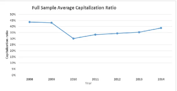
The capitalization ratio average by sector is presented in figure 6 below. The ratio is meas-ured as a percentage and one can detect some specific patterns by studying the lines in the graph. Starting from the year of 2008, it is clear that the majority of the sector’s capitalization rate declined until the year of the IPO, namely 2010. The service sector was the only sector to experience an increase in the ratio, and it is one of the less volatile sectors as seen in the graph. Additionally, one might also conclude that the average capitalization ratios before and after the IPO do not experience any major fluctuations. In contrast, the ratios for the sectors in 2008 spread in a range from 20% to 66%, and in 2014 from 18% to 57%. Hence there was a slight decrease in the range of values when comparing the figures from 2008 and 2014. Furthermore, while examining the graph in 2010, the year of the IPO, it is clear that the values of the ratio are spread within a smaller series of values ranging from 22% to 34% in that year.

Conclusively, it should also be noted that the figures of the capitalization ratio show tenden-cies of being less variable after the IPO, as seen in figure 6 below. This can directly be compared to the pre IPO figures, which illustrate a higher variety and less stable annual values.