Environmental Policies and the EKC
To what extent can national environmental policies contribute to the EKC theory? Sweden and EU
Bachelor’s thesis within Economics
Author: Sanna Efraimsson 19880502
Tutor: Lars Pettersson (Supervisor)
Bachelor’s Thesis in Economics
Title: Environmental Policies and the EKC: to what extent can environmental policies contribute to the EKC theory? Sweden and EU
Author: Sanna Efraimsson
Tutor: Lars Pettersson (Supervisor)
Therese Norman (Deputy Supervisor)
Date: [2012-06-01]
Subject terms: EKC; Environmental Kuznets Curve; Environmental policies; CO2-emission; Environmental taxes; GDP; Sweden; EU
Abstract
The purpose of this thesis is see if national policies regarding aimed at combating climate change could work even if international ones, such as the Kyoto Protocol, are considered to fail. The question was if environmental policies could be included as an explanatory variable for the Environmental Kuznets Curve (EKC). The envi-ronmental polices of interest were the market-based instrument, envienvi-ronmental taxes. First, the hypothesis whether or not Sweden fit the EKC theory is tested, and this proves to be the case when looking at the years 1800-1996. Second, a hypothesis was tested to see if environmental taxes can help decreasing carbon emission intensity further once a country has reached its turning point. Comparing Sweden to six other countries from the European Union show that this is the case, although environmen-tal taxes must be one of many tools and cannot work alone.
The study shows that the role of taxes were significant, thus showing their im-portance for the work on climate change. It is also observed that national policies do work, while regional, or international, ones are harder to conduct. The importance of national policies is enhanced since they will be guiding countries when deciding whether or not to commit to international policies.
Table of Contents
1 Introduction ... 5
2 Policy Background ... 7
3 Theoretical framework ... 10
3.1 The Environmental Kuznets Curve ... 10
3.2 Previous studies ... 11
3.3 Criticism ... 13
3.4 Environmental policies as economic instruments ... 15
4 Empirical Framework ... 17
4.1 Defining variables ... 17
4.2 Methodology ... 19
5 Results and discussion ... 20
6 Conclusion ... 27
Suggestions for further research ... 27
List of references... 28
Suggestion for further reading ... 32
Appendices ... 33 Appendix 1 ... 33 Appendix 2 ... 33 Appendix 3 ... 34 Appendix 4 ... 35 Appendix 5 ... 36 Appendix 6 ... 40 Appendix 7 ... 41 Appendix 8 ... 44 Appendix 9 ... 46 Appendix 10 ... 48 Appendix 11 ... 49 Appendix 12 ... 51
List of Tables
Table 1 Emissions trends of CO2 (million tonnes) ... 8
Table 2 Tax revenue from environmental taxes as share of total tax revenue (million Euros). ... 9
Table 3 Climate Change Performance Index ... 9
Table 4 Output for model 2, 1800-1970, and model 3, 1971-1995 ... 22
Table 5 Elasticities for signigicant output ... 24
List of figures Figure 1 Prices of CO2 allowances from June 2003 to June 2005. ... 8
Figure 2 Kuznets curve ... 10
Figure 3 Structural changes in EKC ... 11
Abbreviations
CO2 Carbon Dioxide COP Conference of Parties CFC Chlorofluorocarbons
CCPI Climate Change Performance Index EEA European Energy Agency
EKC Environmental Kuznets Curve EPA Environmental Protection Agency ETS Emissions Trading Scheme
EU European Union
GHG Green House Gases GLS Generalised Least Squares MAC Marginal Abatement Cost MBI Market Based Instruments
NAFTA North American Free Trade Association OLS Ordinary Least Squares
OPEC Organization of the Petroleum Exporting Countries
OECD Organisation for Economic Co-Operation and Development PPP Polluter-pay-principle
SCB Statistics Sweden (Statistiska Centralbyrå) SO2 Sulphur Dioxide
UNFCCC United Nations Framework Convention on Climate Change
WB World Bank
1
Introduction
The resources of this world are known to be unevenly distributed. This inequality is linked to both the economic development and the environmental development. The goal of economic development, with its attempts to create convergence, is often said to be inconsistent with the goal of environmental sustainability. The goal of sustainability focuses on the idea for current generations to use the resources today while not leaving generations to come worse off; this is true for both economic development and the environment.
The Environmental Kuznets Curve (EKC) is a theory based on the work of Simon Kuz-nets (1955). It links environmental degradation to income (often measured as GDP/capita) resulting in an inverted U-shaped curve. The underlying reasoning is that a country cannot invest in abatement until they have reached a certain level, a turning point, of income. This theory shows that economic growth is not, per se, a threat to the environment. However, the EKC is not a clear cut model but based on empirical observations, hence it does not give much explanation to underlying factors. The EKC gives a good overview on where a country is in terms of abatement, but it leaves many questions unanswered and further ex-planatory variables than income should also be considered.
What generally is looked for when executing these researches are the question whether or not one can observe an inverted-U shape, and also at which level of income there is a turning point in environmental degradation.
The reasoning behind the EKC was first brought to light in the early 1990s. The World Development Report 1992 had the subtopic of Development and the environment, and in this report environmental policies are said to be crucial in order for economic development to happen alongside with environmental sustainability. In 1992 the United Nations Frame-work Convention on Climate Change (UNFCCC) was adopted in order for the interna-tional community to combat climate change, and a rising temperature. The convention works through Conference of Parties (COP) and last in order was the 17th conference held in Durban, December 2011 (UNFCCC, 2012). It is a common belief that these conferences are insufficient. But to what extent does environmental improvements rely on international policies? Can national, or regional, policies show results as well?
International agreements and policies regarding the climate change have been proven to bring desired results. The Montreal Protocol adopted 1987 was a success in combating ozone depletion by bringing down the levels of chlorofluorocarbons (CFCs) in the atmos-phere (US EPA, 2010). However, the success controlling the ozone depletion was an ex-ception of outcome from international agreements. The failure of the Kyoto Protocol and several UNFCCC summits, are often debated in our newspapers. A question raised is whether or not we have the ability to solve the environmental problems on a global arena. From the debate on international policies, it is clear that national policies are given a more important role for a country to succeed in combating the environmental degradation. Multiple international institutions and organisations are every year presenting reports re-garding the climate change. With ambition to increase transparency, the Climate Change Performance Index (CCPI) ranks Sweden at the top out of 58 countries (Germanwatch, 2011). This index is based on three factors:
1. The emission trends 2004-2009; 2. The emissions level 2007-2009; 3. The policy actions for the countries.
What is causing this high ranking? Can it be from differences in national policies that effect emissions?
With a large share of greenhouse gas, CO2-emissions is one of the main contributor to the climate change, in Sweden CO2-emissions is about 78% of the total greenhouse gases (GHGs) (OECD, 2005). There are many economic instruments emanating from environ-mental policies and this paper will compare two of these instruments, environenviron-mental taxes and emissions trading permits, to see if it might enhance the hypothesis of environmental Kuznets.
The aim is to look beyond the EKC curve and see how much of the results that can be ex-plained by national environmental policies. By comparing measurable economic instru-ments to the general EKC curve conclusions can be drawn on how environmental policies affect the EKC. I want to show if Sweden’s environmental policies can be linked to the de-velopment of emission to see if, even though environmental policy-work is failing on the global arena, it might be successful on the national level. By comparing seven countries from the European Union (EU), the aim is to give a picture of what the individual coun-tries are doing, as oppose to incentives from the union itself.
The questions this paper tries to answer are:
First, what are the results of applying the EKC onto Swedish CO2-emissions?
Research hypothesis 1: The EKC theory will be applicable to Sweden and CO2
-emissions will currently be decreasing with an increasing GDP/capita since Sweden will have already reached its turning point.
Second, can the results from EKC theory be enhanced by environmental policies, using
eco-nomic instruments such as trading schemes, and environmental taxes?
Research hypothesis 2: When a country has reached its turning point,
environ-mental policies will further enhance the decreasing CO2-emission.
To see the role that environmental policies play I have chosen Sweden as my country of in-terest. The results of Sweden will be compared to the result for six other EU-countries. Policies can be measured in many different ways but I have choose to measure it by eco-nomic variables. The instruments of focus will be tradable permits, and environmental tax-es. The countries, apart from Sweden, are Finland, Denmark, Germany, the Netherlands, and Italy. The reasoning behind this choice of countries is to compare policies from a few different perspectives. Germany, the Netherlands, France, and Italy are all original coun-tries from the European Coal and Steel Community, and are therefore expected to repre-sent the environmental policies within EU in a good way. Finland and Denmark makes Sweden comparable to our neighbouring Nordic countries, which in many other political areas share the same point of view as Sweden.
After investigating the hypothesis Sweden showed to befitting the theory of EKC. The re-sult of both income and environmental taxes as having a decreasing effect on carbon emis-sion intensity was observed. The result was not consistent for all European countries.
2
Policy Background
The national environmental policy of Sweden is that in 2050 the country should be climate neutral, i.e. net emissions should be zero. The road towards this goal is not yet set, the plan will be finalised in 2013. The step taken to create this plan is emanating from the UNFCCC COP in Cancun 2010 where industrialised countries agreed to come up with long term plans on how to lower emissions (Miljödepartementet, 2012b).
Sweden has 16 environmental objectives, one of these is reduced climate impact, and within this we find the of work combating CO2-emission. This objective has its foundation in the work of UNFCCC; stabilising the GHGs in the atmosphere. Apart from the goal to be climate neutral in 2050, an interim target is set between 2008-2012 where GHGs should be reduced by 4%. Additionally, a milestone target for 2020 is to lower GHG-emissions with 40% (Swedish EPA, 2012).
The two most common economic instruments used by the Swedish government is carbon taxes and emissions trading (Naturvårdsverket, 2011b)
EU’s roadmap 2050 states that EU should lower emission with 80% of 1990’s level by 2050. This commitment will imply new policies since current policies is estimated to only lower emission with around 40%, however these are not specified (European Commission, 2011a).
As a member of EU, Sweden adopts the policies taken at the EU-level, such as the Euro-pean Union Emission Trading Scheme (EU ETS) started in 2005. The EU ETS is a trading scheme for emission where the allowance decreases over time, in 2020 emission allowance will be 21% lower than 2005. As of today, 30 countries participate in the program where Iceland, Liechtenstein, and Norway are additional to EU27 (European Commission, 2010a). The Swedish government is positive to the EU ETS and has a goal of the system to be expanded, and eventually linked to other trading systems (Miljödepartementet, 2012a). The system of ETS is based on the principle of “cap and trade” where there is a total amount of emission permits to be distributed. The total emission of CO2 which is covered within this program is estimated to be around 50% of the emission within the EU (Euro-pean Commission, 2010a). The system is set up in a way so that member countries will be encouraged meet their national Kyoto criteria (European Commission, 2010b). The system is set up in three trading periods between 2005-2007, 2008-2012, and 2013-2015 where for the third period EU is aiming at having half of the allowances auctioned (European Com-mission, 2011b). The first phase had all the permits grandfathered at the national level, the second period had up to 10% auctioned and for 2027 the aim is to have all auctioned (An-dersen & Ekins, 2009). Looking at figure 1 one can see how the prices of permits where changed after the implementation of EU ETS. From 2012 the EU ETS will also include aviation departing or arriving in EU (European Commission, 2012).
Figure 1. Prices of CO2 allowances from June 2003 to June 2005. Source: EEA (2008).
For the EU ETS to be thought of as directing countries in the right direction, if countries emit more than their allocated allowances are considered “good” since this means that there are fewer allowances available than what is necessary to continuing the current level of emissions. In appendix 12 there is a compile of the differences for the seven countries. In Europe, environmental taxes are determined on a national level, this in contrast to EU ETS, which is a regional policy (Andersen & Ekins, 2009). Environmental taxes differs be-tween countries and can therefore be used as a measure for national policies. By con-trasting the effect of environmental taxes towards the EU ETS it is possible to contrast na-tional policies towards regional/internana-tional ones.
How much has already been done?
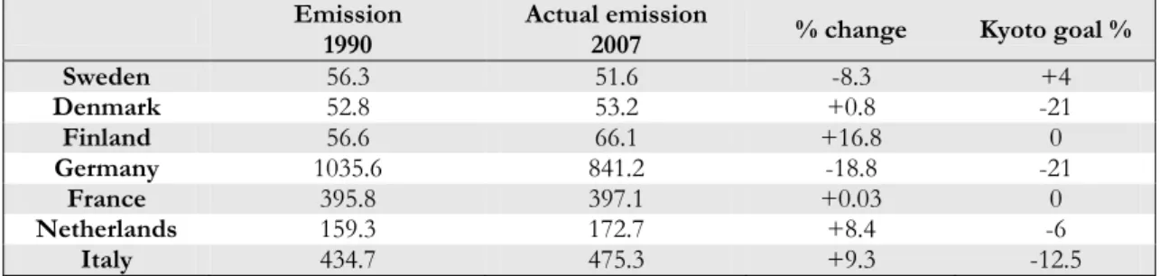
The part goal Sweden to lower emissions by 4% in 2012, compared to the level of 1990, is most likely to be achieved. The emission trend is decreasing since 1996 and the major changes done so far is within the energy sector where oil has been exchanged for district heating, heat pumps, and bio-fuel (Naturvårdsverket, 2011a). The Swedish government has established a motor vehicle tax related to CO2-emission, 2013 the tax on diesel fuel will in-crease, and increased CO2-tax for heating both within and outside the trading sectors (Miljödepartementet, 2012a). In table 1, there is a comparison of the goals and emissions levels for CO2-emisisons for the seven EU countries. It is also shown the breakdown for individual EU members in order for EU to reach the goal according to the Kyoto Protocol.
Table 1. Emissions trends of CO2 (million tonnes)
Emission
1990 Actual emission 2007 % change Kyoto goal %
Sweden 56.3 51.6 -8.3 +4 Denmark 52.8 53.2 +0.8 -21 Finland 56.6 66.1 +16.8 0 Germany 1035.6 841.2 -18.8 -21 France 395.8 397.1 +0.03 0 Netherlands 159.3 172.7 +8.4 -6 Italy 434.7 475.3 +9.3 -12.5
(Source: EEA & EC)
6.00 10.00 14.00 18.00 22.00 26.00 30.00 01-0 7 -20 03 01-0 8-2 003 01-0 9 -20 03 01-1 0 -20 03 01-1 1-2 003 01-1 2 -20 03 01-0 1-2 004 01-0 2 -20 04 01-0 3 -20 04 01-0 4-2 004 01-0 5 -20 04 01- 0 6-20 04 01-0 7 -20 04 01-0 8 -20 04 01-0 9 -20 04 01-1 0 -20 04 01-1 1 -20 04 01-1 2 -20 04 01-0 1 -20 05 01-0 2 -20 05 01-0 3-2 005 01-0 4 -20 05 01-0 5 -20 05 01-0 6 -20 05 01-0 7-2 005 01-0 8 -20 05 01-0 9-20 0 5
Start of EUETS January 2005 EUR
Some main economic instruments used in Sweden for environmental improvements within the goal of reduced climate impact are energy-, and CO2-taxes, tax reductions, reliance and economic support for green technology (Naturvårdsverket, 2007).
Environmental taxes have increased in the EU-15 since 1980, between 1980-2001 the reve-nues from environmental taxes increased by 335%. In absolute terms the revenue of envi-ronmental taxes increased from 54.6 billion Euros in 1980 to 237.7 billion Euros in 2001. This is described as the green tax reform where tax revenues shift towards environmental taxes. Notably, even if the tax revenue from environmental taxes has increased more than other kinds of taxes, as a share of GDP the increase does not seem so significant; going from 2.2 to 2.7% between 1980 and 2001(Johansson, 2003). In table 2 one can see how share of environmental taxes in the total tax revenue has developed from 1990 to 2009.
Table 2. Tax revenue from environmental taxes as share of total tax revenue (million Euros).
1990 1995 2000 2001 2002 2003 2004 2005 2006 2007 2008 2009 Change % Sweden 6.04 5.78 5.35 5.63 6 5.98 5.81 5.79 5.62 5.54 5.77 6.02 0 Denmark 7.44 9.32 10.72 10.78 11.22 10.85 11.45 11.76 12.44 11.97 11.88 9.97 +34 Finland 4.79 6.42 6.64 6.64 6.84 7.24 7.44 7.03 6.88 6.39 6.27 6.17 +29 Germany 5.08 5.85 5.68 6.31 6.37 6.69 6.54 6.35 6.12 5.67 5.57 5.69 +12 France 5.43 6.44 5.58 5.11 5.43 5.3 5.4 5.12 5 4.87 4.79 5.04 -7 Nether-lands 6.86 9.05 9.78 9.85 9.68 9.95 10.28 10.5 10.34 9.82 9.93 10.42 +52 Italy 8.53 8.84 7.42 7.13 6.91 7.05 6.78 6.74 6.42 6.01 5.67 6.08 -29 (Source: Eurostat)
One of many interesting reports and ranking when it comes to the environment is the Cli-mate Change Performance Index (CCPI), which is put together by Germanwatch (2011). This index does not only rank countries after their emission levels but also after their emis-sion trend and climate policy. The rank is a weighted average where emisemis-sion levels ac-counts for 50%, emission trends for 30% and climate policy 20%. Their latest report was published in December 2011 and the countries included in this study were ranked as dis-played in table 3.
Table 3. Climate Change Performance Index
Rank # Country Score Emission Trend Emission Level Climate Policy
4 Sweden 68,1 Good Good Poor
6 Germany 67,2 Good Poor Good
8 France 66,3 Moderate Good Moderate
12 Denmark 63,9 Moderate Poor Good
30 Italy 55,4 Moderate Poor Very poor
37 Finland 53,9 Poor Moderate Poor
42 Netherlands 51,4 Poor Poor Very poor
3
Theoretical framework
3.1
The Environmental Kuznets Curve
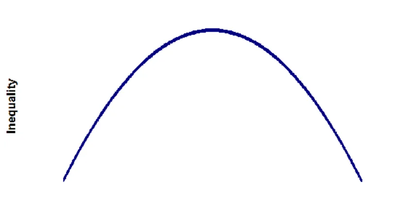
In 1955 Simon Kuznets published an article presenting what is now referred to as the Kuznets Curve. The underlying intention of this paper was to start a discussion on how personal income inequality and economic growth were linked, as presented in figure 2. The theoretical evidence of this article was lacking, however this was also part of the intention: the article’s aim was to show that economics needed to look further into other fields, such as demography. This should be done in order to grasp the linkages between economics and population growth patterns. By looking into fields outside of economics, the economic field itself would develop and no longer be based on too many assumptions (Kuznets, 1955).
Figure 2. Kuznets curve
“Meeting the needs of the present generation without compromising with the needs of future generations” –
this definition of sustainable development, presented in Our Common Future was a starting point for raising public awareness on environment and development (WHO, 1987)
In 1991 the Kuznets curve was developed further, and the EKC was created. Grossman and Krueger (1991) included the relationship between income and environmental degrada-tion in their study on the environmental impacts in Mexico of North American Free Trade Association (NAFTA). In this paper they concluded that after a certain level of income, countries will see diminishing pollution. The authors’ main conclusion on the environmen-tal effects of trade liberalisation was the ones due to policy changes and intersectoral struc-ture changes of economic activity (Grossman & Krueger, 1991). Furthermore they con-clude that economic growth will effect environmental quality through three channels: scale effects, technological effects, and composition effects. The effects from trade on the envi-ronment has been investigated multiple times and it gives both positive and negative effects on the environment. This is in line with trade theory, the Ricardo model based on compar-ative advantages due to technological differences (Brakman et al., 2009).
The World Bank put extra focus on the two-way relationship between the environment and development in the World Development Report 1992, which investigates the relationship between GDP and environmental degradation over time, although not through the termi-nology of EKC (WB, 1992). This report claims policies are an additional source next to economic growth for countries to solve the environmental problems. The government level is the main force in environmental issues since private market provides insufficient in-centive to engage. The policies taken by a government can be aimed towards both goals, and environmental policies can be used to complement and reinforce development.
The report comment on following to have respective impacts on the environment: - Economic policies: affects scale, composition, and efficiency of production. - Environmental policies: reinforce efficiency and provide incentives to adopting
less-damaging technologies.
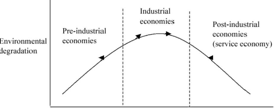
Above concludes into one of the main findings of the EKC theory: a rising income will create a greater demand for improving environmental quality (WB, 1992). Additional to the greater demand for environmental improvements that arises alongside with increasing in-come, is also the explanation that environmental improvements from structural changes. Structural changes that follows from economic growth implies changes in pollution levels as the economy moves from clean agrarian production, to polluting industry, and finally to a clean service sector (Ciegis et al., 2007). This structural differences will directly affect the pollution levels and can therefore bring a somewhat skewed result of the EKC between developing and developed countries. As theories of trade predicts, developing countries are more likely to engage in production based on natural resources and labour while developed countries are more likely to engage in the less-pollution-intense service sector (Hettige et al., 1992).
Fig 3. Structural changes in EKC (Source: Panayotou, 2003)
Even though the EKC hypothesis often is supported by empirical research, it is not the economic growth itself that leads to environmental improvement but the contents of growth; the inputs and the outputs, which in turn is a result of institutions creating incen-tives (Arrow et al., 1995).
3.2
Previous studies
There are numerous studies on the relationship between income and pollution explained by the EKC theory. Using many different explanatory variables, different scholars have found
the result of turning point to be widely spread, and the numerical value of this turning point will not be the focus in this paper.
One of the main contributors to the work on the Environmental Kuznets Curve is Stern who reviews the theory several times. In one of these, Stern (2004) provides 4 factors to the EKC: 1. Scale of production 2. Output mix 3. Input mix 4. State of technology: - Production efficiency
- Emission specific changes in production
There are numerous underlying dynamics that will determine these factors: education, envi-ronmental regulation and awareness are a few of these. These dynamics are also what is linked to a fairly high level of income. Thus, confirming the EKC hypothesis.
In a special review of the EKC, Barbier (1997) concludes that the early work on EKC fo-cuses much on the structural changes and the composition of goods & services. However, the changes in environment-income linkages are not only exogenous but depend also in endogenous policy changes (Barbier, 1997). Barbier lists the main relationships underlying the EKC where he moves the theory closer to the role of environmental policies compared to Stern (2004):
- Structural economic change plays a crucial role; - Income and demand for environmental quality; - Local versus global pollution;
- Country specific effects:
- The role of national and local policy;
- The role of multilateral policy.
One of the first to implement policies as a variable into the EKC empirical research was Panayotou (1997) when looking into SO2-emissions. The EKC is a potential “black hole”, which Panayotou describes as “it hides more than it reveals since income level is used as a catch-all
surrogate variable for all the changes that take place with economic development” (Panayotou, 1997). An
attempt is to get around this potential problem by including policy as a variable together with the rate of economic development.
Adoption of proper policies and property rights can change the steepness of the EKC, and thereby lower the turning point. In his paper investigating the EKC for SO2-emission, Pa-nayotou identifies three determinants for environmental quality: 1. The scale of economic activity; 2. The composition of economic activity; 3. The effect of income on demand and supply of pollution abatement effort. The latter is his contribution to the theory of EKC. The policy variable used by Panayotou is chosen from a composition of five indicators for institutions in general, where Panayotou used respect/enforcements of contract. The finding is that policies might results in positive effects that will offset the negative effects on the en-vironment from economic growth and population density. This is true both for low income and higher income countries, but will have a larger impact on higher income levels since higher income levels are required for abatement to take place (Panayotou,1997).
Including policies as a variable have shown to effect the turning point. Further studies with policies as a explanatory variable has been made by creating a dynamic model. A simulation
of this, made by Anderson & Cavendish (2001), shows how the time of implementing a policy will result the turning point for CO2-emissions in the energy sector. The study tries to go further than relating CO2-emission to income and therefore explains the effect by policies (resulting in technological process) exogenous of income. The reason for this is the fact that the turning point for CO2-emission ranges from 13’000$ - 35’000$ depending on explanatory variables in the EKC (Anderson & Cavendish, 2001).
Technological progress is true for developed countries but hardly for developing countries and this studies tries to show how time is a determinant for policies to give result. The simulation shows that for developing countries, with an initial GDP/capita of 2’500$ and a growth rate of 4%, the peak levels of emission of the EKC will decrease by two thirds, and the turning point will be half a century earlier from en early implementation of policies compared to a 100-year delayed “no policy” (Anderson and Cavendish, 2001 fig5). The main benefit from implementing environmental policies is the incentive for technolog-ical progress and this simulation also found that even though there is a lag between imple-mentation and effect of a policy, it is not as long as what is usually the result of an EKC. Policies are often used as a way to internalise the externalities.
In general, some economic instruments for managing the environment are to remove dis-tortionary subsidies, secure property rights, pollution taxes, user charges, tradable emission permits, and refundable deposits (Panayotou, 1994). Panayotou describes economic in-struments as an aim to bridge the gap between private and social costs. The key to success lies in creating incentive and “economic instruments in effect transfer from bureaucrats to the market
the responsibility of identifying and exploiting new and additional low cost sources of pollution control“
(Panayotou, 1994 p5).
Scrutinising result from the EKC a drawn conclusion is that in most cases where emission decreases with income this is due to local institutional reforms, such as environmental legis-lature and market-based incentives to reduce environmental impacts (Arrow et al., 1995). Unfortunately these often ignores the international consequences leading to environmental dumping; when countries with harsh policies and regulations move production to develop-ing countries where environment is hardly considered in legislation. Even if there are downturns, environmental policies is a must alongside economic growth. Institutions are necessary in order to create incentive for the resource users (Arrow et al., 1995).
3.3
Criticism
The EKC is fairly criticized by many authors. One critique is that the statistical analysis is not sufficient enough to build the EKC hypothesis upon. The arguments for this critique is that the EKC is not a common observation for different countries and different pollutions (Stern, 2004). There are many underlying factors deciding whether or not a country will fol-low the inverted U-shaped EKC; depending on which explanatory variables, and also which dependent variable, one chose.
In his paper Progress on the EKC?, Stern (1998) summarises the main critics of the EKC drawn from a previous article (Stern et al., 1996). There are seven major problems with the EKC, and some of them have been reconsidered already:
1. Simultaneity and irreversibility
We might see a relation between our dependent variable and the error term, simultaneity bias which might occur when policies on emission will create a feedback to our explanatory variable (Holtz-Eakin & Selden, 1992). The issue of simultaneity has been addressed by
Holtz-Eakin and Selden in 1992, by using Hausman test for regression exogeneity they did not find any simultaneity. The problem of irreversibility is due to the fact that EKC theory is based on the assumption that environmental degradation will decrease with a rising GDP/capita. However, at some point emissions are irreversible, we cannot fix the problem already caused.
2. Trade and the EKC
Most papers investigate the openness to trade and not the trade flows itself. The problem arises when looking into trade theory; trade will lead countries to produce according to comparative advantage. This will enhance the EKC results when poorer countries special-ise in pollution intense activities.
3. Ambient concentration versus emission
Early studies of EKC used ambient data from urban areas. However, ambient concentra-tions will follow the development of urban population density, which tends to increase and then decrease with time. This problem has now been straightened out by the use of emis-sion data instead, also resulting to higher turning points.
4. Asymptotic behaviour
No matter how much a country improves according to the EKC theory, economic activity will always be associated with some kind of waste hence it is inappropriate to have a regres-sion where levels can become negative.
5. Mean versus median income
Using a mean income might give skewed results. Using the median income would be better since there are more people living below the mean income than above it. However this is a data problem since GDP/capita is easier to estimate than median values.
6. Aggravation and other environmental problems
While some pollutants have in fact decreased as the EKC implies, others may have in-creased and total pollution might be the same, or in fact increasing. This problem has been raised by not only by Stern. It is extended by Arrow et al (1995) and they state that the EKC might only be applicable to short-term, local pollutants such as sulphur, while global pollutants, CO2 especially, will not be fitting the inverted U-shape. It is estimated that CO 2-emissions will in fact have an N-shaped curvature instead. Indicating that at first we will see the structure of an inverted U but after certain levels of income, the emissions will increase again (De Bruyn et al., 1998). The reason is that at this level of income where the relation to environmental degradation becomes positive again, the technological improvements etc, has been exhausted. However, De Bruyn et al. favours the inverted U-shape over the N-shape since it has been observed more than the N-N-shape.
7. Econometric problems
Stern believes in the empirical result showing that the relationship building the EKC is there, however there is a lacking econometric foundation in the literature dealing with the hypothesis. One critic is raised to the use of cross-sectional data, instead of panel, since many of the countries used are located in parts of the world here more heating is required, the result might be a bit skewed (Holt-Eakin & Selden, 1992).
Additionally, there is a need to look at historical events when investigating the theory of EKC. An example is the oil crisis in 1973, which explains some of the decreasing pollution at the time apart from an structural changes (Moomaw & Unruh, 1997). Furthermore they
claim that much data, which EKC investigations are based on are from after 1970’s and do not capture the decreasing emission before then. Stern (1998) provides a short summary of econometric techniques used when looking into the EKC relationship. They are widely dif-ferent; ranging between cross-section, panel data, times series and using different estima-tion techniques such as OLS, GLS, Fixed effects, Random effects etc. Also the dependent variables differs from logs, to levels and “change” logs.
3.4
Environmental policies as economic instruments
The importance of policies have been proved through various empirical research but what is underlying the structure of policies?
How environmental policies are conducted can be explained by the role of the state over history. An example from the United States and United Kingdom looking back at a welfare state in the 1950-60’s the command-and-control policy was in use, while in the 1970’s the welfare state diminished as did the command-and-control move towards market based pol-icies (Hepburn, 2010). State intervention can be put on a scale ranging from:
With the free market on one side of the spectrum, and nationalised delivery on the other, it is of general belief that the solution lies somewhere in between since the extremes are likely to result in market failure respectively governmental failure (Hepburn, 2010).
Two main reasons to why a free market can protect the environment is first the demand from consumers; being well-informed about environmental issues and wanting to combat them, firms will have to meet customer preferences. Second, firms will make profits by do-ing so and therefore an incentive is created (Hepburn, 2010). However, these incentives are not strong enough and CSR policies from firms needs to be complemented by government action (Reinhardt & Stavins, 2010).
A free market is insufficient to protect the environment due to three central explana-tions: 1. Environment is considered external; 2. The problem of public goods; 3. The prob-lem of common goods (Cato, 2011).
When firms see the environment as external they will not include the cost of pollution within their accounting and hence the price charged will not cover the real cost. In the case of common goods, the problem can be defined as through the tragedy of the commons; if a good is non-excludable but rivalrous, then peoples’ desire to use the resource will lead to over-exploitation (Hardin, 1968). While a common good is rivalrous, a public good is not and climate protection is a pure public good. Hence it creates a reluctance to engage in pro-tection since gains can be used by everyone and not only the paying party (Hanley et al., 2007).
When the market fails to protect the environment, the government intervenes by imposing taxes, emissions standards etc. The need for government intervention shows that the Coase
theorem is inconsistent; zero transactions costs is not the case and interventions is necessary
if a Pareto efficiency should be achievable (Hanley et al, 2007). A world of zero transactions cost was not considered achievable even by Coase himself, and instead it is necessary to look at a world of incomplete markets (Coase, 1960).
Imperfect economies comes from the impossibility to have perfect information re-garding the price of environmental degradation, and rent-seeking behaviour of government
Free market Information Provision Moral suasion Economy-wide relative prices Output-based intervention
Input- or technology-based
intervention
Project-level
employees. This rent-seeking behaviour is explained by the principal-agent problems; when government representative have something else in mind than social optimum, government intervention is likely to fail (Stiglitz, 1987).
By creating incentives for firms, and individuals, to engage in environmental protection, governments can combat the above explained problems. Incentive systems can provide flexibility of adoption but will encourage actions towards desired public objectives. The main reason for market-based instruments is to find an alternative to the command-and-control policies that usually is used for environmental protection (Hanley et al., 2007). Market-based instrument is aimed at internalising the externalities. When the market fails to protect the environment, the government intervenes by imposing taxes, emissions stand-ards etc.
Government intervention can be viewed to be non-optimal; imperfect economies comes from the impossibility to have perfect information regarding the price of environmental degradation, and rent-seeking behaviour of government employees. This rent-seeking be-haviour is explained by the principal-agent problems; when government representative have something else in mind than social optimum, government intervention is likely to fail (Stiglitz, 1987).
Decentralised policies are such as liability laws, property rights, moral suasion, and green goods. Centralised policies are environmental standards, such as command-and-control policies (Olewieler & Field, 2011). In between we find the incentive policies working as market-based instruments (MBI); taxes, subsidies, and transferable emissions permits. The way these works is by the government setting an objective and then leaves it to the market to reach this goal. One description is to design an incentive system with private flexibility that will achieve public desires (Hanley et al., 2007). The way to internalise externalities is to create a cost higher than a company’s marginal abatement cost (MAC) since this will create the incentive to change emitting by investing in abatement. MBI are sometimes defined as the “polluter-pay-principle” (PPP) by many governments, EU and Sweden are both users of the principle when legislating. The PPP will prevent the environment from being mis-used as a common good since it is creating incentives for polluters to become environmen-tally friendly. An underlying idea is that environmental policy cannot be effective if it is de-tached from other policy areas, and the PPP therefore links it to fields like transport, and agricultural policies (Knill & Liefferink, 2007).
Comparing environmental taxes and trading from this perspective there is a difference. While taxes fix price and lets quantity adjust, trading permits fixes quantity and lets price adjust (Andersen & Ekins, 2009). Critical ingredients for policy to be effective are the en-forceability and incentives for innovation (Olewiler & Field, 2011).
4
Empirical Framework
This section will describe the foundation of the model used in this thesis as well as the var-iables used.
The classical model when conducting research on the EKC is one described by Stern (2004);
ln(E/P)it = αi + γt + β1ln(GDP/P)it + β2(ln(GDP/P))2 it + ε it
The dependent variable here is a emission (E) per capita (P) and the explanatory variables are GDP per capita (P) and GDP per capita (P) squared. The model is constructed for a panel data set and used logged variables. This model by Stern, where GDP2 is included is suitable for longer time periods where there is nonlinear relationship. Along the way is has been clear thatthe shorter time series data in this thesis are not suitable for GDP2 and therefore this property has been removed. Unlike Stern’s framework, the dependent varia-ble will be a ratio showing the carbon emission intensity, which is similar to the dependent variable as used by Roberts & Grimes (1997). This will create a dependent variable that is less sensitive to production fluctuations. Furthermore, the variables will not be used in their logged form since they will be transformed by taking first difference, and using logged variables additional to this will remove some of the information in the variables.
4.1
Defining variables
NOTE:
All variables are measured as per capita. All data is annual data.
Dependent variable
( ) CO2/capita over GDP/capita, estimating the emission intensity.
The ratio of CO2-emissions per capita over GDP per capita will consider the production fluctuations from different events, such as economic crises, and represent the intensity of carbon emissions in a country.
CO2
The data used for hypothesis 1, 1800-1995 comes from The State Price and Competition Agency (cited by Kander, 2002) and is measured in metric tonnes. For hypothesis 1, 1990-2009 data is retrieved from Eurostat and carbon dioxide is measured as thousands of tonnes.
GDP
Data used for hypothesis 1, 1800-1995 comes from Historical Statistics of Sweden and the value is measured with 2000 as reference price and measured in SEK. For hypothesis 2, 1990-2009 GDP is reported by Eurostat in current prices, adjusted for PPP and measured in Euros.
Explanatory variables
( ) GDP/capita
( ) GDP/capita, squared
( ) Total revenue from environmental taxes per capita
( ) Revenue from Energy-related environmental taxes per capita
( ) Revenue from Transport-related environmental taxes per capita
( ) Revenue from Pollution-related environmental taxes per capita
Environmental taxes
Environmental taxes have been defined by the OECD ”A tax whose tax base is a physical unit
(or a proxy of it) of something that has a proven, specific negative impact on the environment” (Eurostat
& SCB, 2009 p3). Furthermore Eurostat distinguish environmental taxes from fees or charges by defining environmental taxes as compulsory payments where the benefits pro-vided to the taxpayer are not directly linked to the payment. This compared to fees, or charges, where the benefits are directly linked to the payments.
Division of environmental related taxes have been categorised in four categories by the Sta-tistics Sweden (SCB), and the same definition is used by Eurostat where the data has been collected.
It is energy, transport, pollution, and resources. The environmental taxes in this data set Eurostat has gathered pollution and resources into one category. The total tax revenue will be included as an explanatory variable in the regression model, and the three categories will be subject of a graphical comparison between the seven countries.
Energy taxes: includes both stationary (fuels oil, natural gas, coal, and electricity) and
transport (petrol, diesel, etc.) used energy products. To note is that this category include the taxes on CO2 since these taxes are partly substituting taxes for other energy sources.
Transport taxes: this category includes the taxes on motor vehicles. Such as ownership and
import/export/sales of equipment. Also, road taxes are included here but not taxes on transport fuels, which is included under energy.
Pollution taxes: Measured or estimated emission to air, water, along with management of
sol-id waste and noise. Note; CO2 taxes are categorised as energy taxes.
Resource taxes: these are taxes on extraction of forest, mining, oil, gas, and water
consump-tion.
the categories (transport, energy, and pollution&resources) the data cover years 1995-2009. The unit of measure for environmental taxes are specified as millions of euros.
(Source: Eurostat, metadata)
4.2
Methodology
To investigate research hypothesis 1 I will first create a scatter plot to graphically see if the the-ory of EKC can be applied to Sweden. Secondly, running an OLS regression for emissions intensity and GDP/capita for Sweden over time will show if the theory of EKC can be proven significant.
Moving on to research hypothesis 2 I will look at the seven EU countries between 1990-2009. For these seven countries individual time series will be constructed to first see the signifi-cance of the GDP, and thereby investigate the EKC theory for each country. After that the impact of environmental policies on carbon emissions intensity will be investigated by us-ing environmental taxes as an explanatory variable. This will be done first by usus-ing the ag-gregate level and then using the categories of different environmental taxes.
- Tax revenue from environmental taxes
- Tax revenue from categories of environmental taxes
Since the EU ETS was set up 2005 indicating that for this paper the data is only covering 5 out of 20 years. Therefore it will not be include as an explanatory variable when running regressions. It will instead be considered theoretically since it makes a good ground for comparing national and regional/international policies.
5
Results and discussion
Research hypothesis 1: The EKC theory will be applicable to Sweden and CO2-emissions will cur-rently be decreasing with an increasing GDP/capita since Sweden will have already reached its turning point.
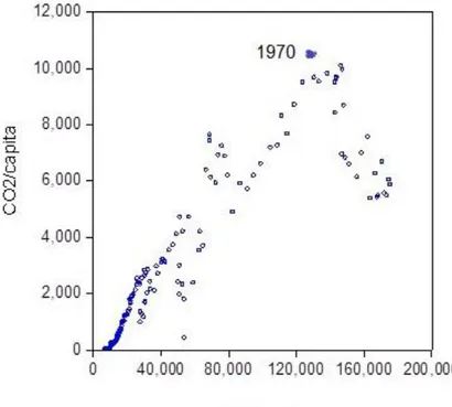
First, to see if a relationship exists between CO2-emissions and GDP a graphical interpreta-tion will be made; creating a scatter plot of CO2-emissions/capita against GDP/capita for Sweden between 1800-1995 one can see that it follows the suggested pattern of the EKC theory.
Fig 4. Relationship between CO2 and GDP in Sweden 1800-1995
Looking at figure 4 one can see an inverted U-shape as theorised by the EKC. The turning point observed in figure 4 is the year 1970. All points left of that represent years before 1970 and all point right of that represents years after 1970.
When looking at the EKC it is important to note underlying historical facts. It is not just GDP and CO2-emissions that should be reflected upon but the error term captures im-portant historical events that might explain some of the results. When looking at Sweden, the plots represented in the lower left corner with low CO2-emissions and low GDP per capita are all years before 1920, which can be linked to the industrialisation which in Swe-den happened during the 19th century (Corell & Söderberg, 2005). Between 1930-1975 the industrialised society was at its top – with some exceptions during WWII. During this time the world was experiencing increasing transport, production etc., and with this came the in-creasing emissions. Up to 1970’s the Western world became more and more dependent on fossil fuels. The observed turning point for Sweden was in 1970. Contributing factors at that time was the OPEC-crises, and increasing nuclear power in Sweden. Other policy-related events that can be linked to the observed turning point are; the implementation of
Swedish EPA (Naturvårdsverket) in 1967, the Swedish Environmental Protection Act (Miljöskyddslagen) from 1969, the Stockholm conference in 1972, more focus on econom-ic tools during 1990’s, and the implementation of the Environmental code (miljöbalken) in 1999 (Forsberg, 2002). The decreasing CO2-emissions compared to GDP/capita since 1970 is described as a delinking explained by above reasons, and also by productivity changes (Lindmark & Andersson, n.d). It is also partly explained when Western economies moved from Fordism into Post-Fordism; moving from mass production into smaller scale, specialised production where innovation plays a large role (O’Brien & Williams, 2010). Graphically, Sweden is falling under the category of “post-industrial economies” as de-scribed in fig 3.
Looking at figure 4 it is clear that in order to create valid regressions one must distinguish the years before 1970 from the years after 1970, due to their non-linear relationship. This is done by creating two data sets and run regressions separately.
1. 1800-1970 2. 1971-1995
When working with time series one should look to see if the model is stationary or not. In order to see this, a graphical examination is a good way to start. For the entire time series, 1800-1995, displaying both GDP/capita and CO2-emissions/capita respectively over time the variables shows signs of non-stationary (appendix 1). Additionally to a graphical exami-nation, one can conduct a unit root test (appendix 2). This test confirms that the there is a trend over time for both CO2 and GDP/capita respectively resulting in non-stationary da-ta. Since the data is non-stationary, in order to be able to draw accurate conclusions from OLS regression one can take the first difference for the variables included to solve for the non-stationary problem and transform the data to become stationary. However, conducting an Engle-Granger test it is shown that the variables are cointegrated at I[1] and hence there is no need to take first difference.
Doing the same for respective period, one can graphically suspect non-stationary data for both (appendix 3). The non-stationary is confirmed when conducting a unit root test (appendix 4). However, conducting an Engle-Granger test for both time periods one can see that both GDP/capita and CO2/capita are cointegrated at I[1] for 1971-1995, hence no need to take first difference. However for 1800-1970 this is not the case and first difference will be taken.
Additionally for 1800-1970, GDP2 will be added as a variable since this period shows an exponential pattern compared to the linearity for the period 1971-1995 (appendix 3). The models will therefore be:
Sweden 1800-1970
D( )t= β1 + β2D( )t+ β3 D( )t2+ ε (Eq. 1)
Sweden 1971-1995
The output from running regressions on model 2 and model 3 can be seen in table 4.
Table 4. Output for model 2, 1800-1970, and model 3, 1971-1995.
Looking at the coefficients one can indeed see that up to 1970 an increasing GDP/capita resulted in increasing intensity of CO2-emissions. Calculating the elasticity one can see that on average when GDP increases 1%, emission intensity increases by 6.653%, which is ex-plained by the vast development during the industrialisation. Respectively after 1971 an in-creasing GDP/capita results in dein-creasing intensity CO2-emissions. The elasticity here ex-plains that on average when GDP increases by 1%, the emission intensity decreases by 1.044%.
Econometric notations:
The models have been tested for normality, autocorrelation, and heteroscedasticity in re-siduals and noteworthy is that for Sweden 1971-1995 the model do experience some auto-correlation.
Thus, hypothesis 1 is confirmed. There is a pattern resembling EKC in Sweden over time, the turning point is 1970 which is represented as the highest point in the scatter plot.
Research hypothesis 2: when a country has reached its turning point, environmental policies will fur-ther enhance the decreasing CO2-emission.
To look into research hypothesis 2, regressions will be run for separate time series of the seven countries between 1990-2009 in order to see whether environmental taxes and ETS have an impact on carbon emission intensity. To draw conclusions on the importance of envi-ronmental policies for Sweden, six other countries will be investigated in order to support the results.
Creating correlation matrices for each time series it is easy to conclude that there is multi-collinearity present (appendix 5). By conducting a unit root test for all time series it was ob-served that the data is non-stationary. If having non-stationary data it is likely that our re-gression will be spurious, they might be significant even if they are not. For both problems, one remedy is to transform the variables by taking first difference. The Engle-Granger
ap-Sweden 1800-1970 Equation 1 Coefficient (t-stat) GDP Elasticity Coefficient (t-stat) GDP2 F-stat Adj R2 0.000000444 * (4.814992) 6.653 0.000000000011 * (-3.076403) 15.61279 0.147436 Sweden 1971-1995 Equation 2 Coefficient (t-stat) GDP Elasticity Coefficient (t-stat) GDP2 F-stat Adj R2 -0.000000103* (-10.92821) -1.044 119.4258 0.831491
proach also concluded that the variables are not cointegrated, hence the need to take first difference is confirmed.
However, taking first difference proves to create insignificant results from the re-gression, confirming the suspicion of spurious regression above but can also be due to the fact that taking first difference makes one lose some of the long-run relationship between the variables. Likewise, the time series used are short and this enhance the consequence that transforming the data will take away information. It is thereby so that the problem of multicollinearity is not always suitable to fix for (Gujarati & Porter, 2009).
Regressions output will be presented both with and without first difference. As the theory of EKC suggests an inverted U-shape, including GDP is usually done twice, one where it is normal and one squared, when running regressions. However, dealing with comparison between countries and national policies, a short time span 1990-2009, and a span with years when the turning point has already been passed; which is assumed to be correct for all seven countries. It is not the potential inverted U-shape that is investigated but whether or not environmental policies (through environmental taxes and ETS) have an impact on CO2-emission levels. During the span 1990-2009 the relationship is linear. To compare Sweden to other countries regarding into research hypothesis 2, the models will move away from the model by Stern (2004).
Looking into research hypothesis 2, GDP2 will be excluded.
Moving into the comparison between Sweden and other EU members there will be 3 vari-ables interpreted and their impact on CO2 intensity. Each of these variants will also be done with first difference. Hence six different regressions will be run for each country. It is concluded that rising GDP/capita is in fact followed by a decreasing CO2 -emissions/capita in Sweden since 1970., i.e. carbon emissions intensity is decreasing. The first thing will now be to estimate this relationship for each individual country to see if the theory of EKC is valid for all countries.
( )t= β1 + β2 ( )t+ ε (Eq. 2)
D( )t= β1 + β2 D( )t+ ε (Eq. 3)
Once this is done, new regressions will be made where total tax revenue for environmental taxes is the explanatory variable in order to the effects of environmental policies on carbon emissions intensity. When estimating each country individually in time series regression it is possible to see the impact from environmental taxes and how the result differs between the countries.
( )t= β1 + β2 ( )t+ ε (Eq. 4)
D( )t= β1 + β2 D( )t+ ε (Eq. 5)
After this is done an additional regressions will be run in order to see if there are any cate-gory of taxes that proves to be significant. Doing so it will be easier to interpret the effects
of specific taxes and one could also see the differentiated production structures between the countries of interest (appendix 11).
( )t= β1 + β2( )t+ β3( ) + β2( ) + ε (Eq. 6)
D( )t= β1 + β2D( )t+ β3D( ) + β2D( ) + ε (Eq. 7)
Looking at the VIF (appendix 6) it is clear that by using first difference one solve for the multicollinearity but also removes the significance of the explanatory variables (see appen-dix 7). The suspected reason for this is the sample size; the fact that the time series is only 20 years, and for taxes it is only 15 years. When then taking first difference one solve for the statistical problems but one also loses much of the information and the output shows to be insignificant.
Interpreting the regression output (appendix 7) with this in mind one can comprehend some things regarding the role of income and environmental taxes on the trend of carbon emissions intensity. For the significant output from equation 3 and equation 5, the coeffi-cients have been recalculated to its elasticities in table 5.
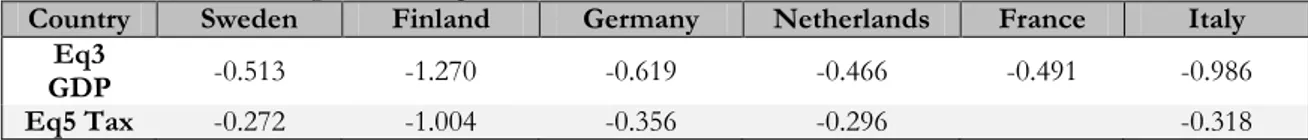
Table 5. Elasticities for significant output
Country Sweden Finland Germany Netherlands France Italy Eq3
GDP -0.513 -1.270 -0.619 -0.466 -0.491 -0.986
Eq5 Tax -0.272 -1.004 -0.356 -0.296 -0.318
The output of equation 3, with first difference, shows that GDP/capita is explaining a de-creasing carbon emission intensity, with the exception of Denmark and France. This signif-icance of GDP shows that the theory of EKC is consistent for Sweden, Finland, Germany, the Netherlands, and Italy. Looking at the emission intensity (appendix 8) for all countries during this time span this is confirmed. The carbon emission intensity (appendix 8) seems to be decreasing even for France and Denmark but this cannot be explained statistically. The result from regression might be due to a short time series but it also indicates that the-se two countries does not perform as well combating climate change as they should. The elasticites (table 5) also confirms that carbon emission intensity will be decreasing with an increasing GDP. For Sweden this means that on average when GDP increases by 1%, car-bon emission intensity will decrease by 0.513%.
For Sweden, equation 3 confirms the findings from hypothesis 1; the country has reached its turning point and is following the theory of EKC.
The significance of taxes on carbon emission intensity is also true, with the exception of Denmark, France and the Netherlands. For Sweden, Finland, France and Italy taxes proves to be significant for carbon emission intensity by running regression on equation 5. The elasticities (table 5) shows that taxes does not affect the carbon emission intensity as to the same extent as GDP but it does have impact. For Sweden it shows that when tax revenue from environmental taxes increase by 1%, carbon emission intensity decreases by 0.272%. The result shows that MBI do have effect on emissions, and using environmental policies where the cost is moved onto the polluter is meeting the intentions of the concept; inter-nalising the externalities. However, the tax revenue has not increased much as share of total
taxes (Johansson, 2003) and could be implemented to a greater extent if a green tax reform can be observable.
Equation 7 results in the category levels of taxes to be insignificant, and thereby category levels of taxes cannot be interpreted. The data on categories of taxes only covers years from 1995 which results in time series with only 15 observations, and this will not yield re-liable results.
Comparing the result for taxes estimated by regression output to the CCPI conducted by Germanwatch one can see some resemblance. For both Sweden and Germany, both ranked relatively high according to the CCPI, GDP and taxes were both of significance also when taking first difference creating a stronger model. This indicates that the countries are performing well regarding climate change. Also Italy and Finland indicated significance of GDP and taxes for CO2-emissions. If comparing with the tax trend (appendix 9) one can see that Italy has not had any significant change in their tax revenue from environmental taxes. Linking this to the CCPI enhances their ranking as performing poorly with their cli-mate policy. One result from this study that goes against the CCPI is Finland’s; the country seem to perform better than their ranking and environmental taxes are of significance, looking at their constant emission level it is likely the that the carbon emission intensity might be overlooked by the CCPI.
When comparing the role of national policies to regional/international ones, the EU ETS is a good comparison for the countries in this study. There are various reviews of the sys-tem which compares it to other economic instruments and also critique from a political view. One of these papers (Helm, 2009) argues that the ETS is not as good as carbon taxes due to several reasons; the system is only planned up to 2020 and this lack of long-term thinking is making the system vulnerable; , the system can drive up permit prices to high up to a point where they are volatile (Helm, 2009). This statement can be linked to figure 1 where it is clear that prices of permits has increased since the system started. A last com-ment noteworthy is that the system is in the target of lobbying; companies would obviously like to keep a grandfathering of permits (Helm, 2009). In this sense, a carbon tax is prefer-able.
Looking at the seven countries during the two first periods (appendix 12): Sweden, the Netherlands, France, and Finland has emitted less than allocation, while Denmark, Germa-ny and Italy has emitted more than allowed by allocation. Considering that EU has a goal that permits should be following the Kyoto protocol and result in a lowering of emission, it is viewed as bad if a country uses less permits than what has been allocated since the sys-tem is supposed to create incentives. Interpreting this one can see that Sweden, the Nether-lands, France, and Finland has all allocated too many permits among their companies, while Germany, Italy and Denmark has created incentives for their markets to lower emissions. The system should create scarcity of permits in order to be successful. Considering the re-sult from Andersson & Cavendish (2001) it might still be considered good that the system was started in 2005 although not structured perfectly since time of implementation proves to be significant for decreasing CO2-emissions. It is hard to estimate the success yet due to three reasons: 1. The incentives to lower emissions will come as the total allowances dimin-ishes yearly; 2. allowances were distributed too generously when implementing the system; 3. the low part of auctioning within the first two periods since grandfathering does not set enough pressure on companies to start lower the emissions.
Summing up it is clear from hypothesis 1 that Sweden does fit the theory of EKC, and moving beyond income as the explanatory variable it is also shown that after the turning point environmental policies, such as environmental taxes, do have an effect on carbon emission intensity. When comparing to the other countries the role of environmental poli-cies shows to differ between the countries and this result confirms the previous investiga-tion by Germanwatch (2011).
6
Conclusion
The theory of EKC is applicable for Sweden between the year 1800-1995. Sweden reached its turning point of emission in 1970 and the country has since experienced a decreasing carbon emission intensity with an increasing income.
Looking at Sweden between 1990-2009 and comparing with six other countries from the European Union it is shown that for income as an explanatory variable the majority of countries follow the EKC theory. The same goes for environmental taxes as explanatory variable; indicating that using market-based instruments as environmental policies do work. It is also clear that environmental taxes alone cannot be a determinant for fighting climate change, since the results in this paper were different for each country it shows the signifi-cance of including other economic instruments as well. Furthermore, environmental taxes does not show the same significance as GDP but the result from taxes can easier be used for policy implications. Comparing the result from this paper with the CCPI from Ger-manwatch (2011) on climate performance one can see that result for each country is rough-ly corresponding the overall ranking of environmental policies.
The trading scheme itself is hard to compare empirically to national policies. The ETS will most likely show some result after the third period which should not be seen as a failure since a system like this would be more likely to fail if being to restricted in the beginning. There is a large possibility that the ETS can be explained indirectly by policies; countries have different general attitude towards ETS due to different green policies from their gov-ernments.
When comparing national to regional policies, national policies will be a determinant for the success of regional (or even international) policies. This can be linked to the studies of Panayotou (1997) where respect/enforcement of contracts were included. National policies have formed national legislation and this will likely be used as a ground when taking standpoint in debates on the international agenda.
The output from this research confirms the hypotheses investigated are valid for Sweden; both income and environmental taxes contributes to a decrease in carbon emission intensi-ty. Sweden might be good from a Kyoto perspective where emissions are decreasing far more than what is expected due to their goal for 2012. However, Sweden could improve their environmental policy further and especially environmental taxes which has not sub-stantially changed as share of total tax revenue since 1990.
Suggestions for further research
The regression output on categories of taxes roved to be insignificant in this thesis. When looking the output to the individual trends of emissions and taxes (appendix 8) one can be-lieve a relationship do actually exist and this calls for further research. By gathering data over longer time periods once could perhaps see some specific effects of certain environ-mental taxes on CO2-emissions. This should also be done in the light of sectoral emissions (appendix 11) in order to use the results for policy suggestions.
List of references
Anderson, D., & Cavendish, W. (2001). Dynamic solutions and environmental policy anal-ysis: beyond comparative statics and the environmental Kuznets curve. Oxford Economic
pa-pers, 53, 721-746.
Andersen, M.S., & Ekins, P. (2009). Carbon-energy taxation. Oxford, NY: Oxford University Press.
Arrow, K., Bolin, B., Costanza, R., Dasgupta, P., Folke, C., Holling, C.S., Jansson, B.O,. Levin, S., Mäler, K-G., Perrings, C., & Pimentel, D. (1995, April 28). Economic growth, Carrying capacity, and the environment. Science., 268, 520-521.
Barbier, E.B. (1997). Environmental Kuznets Curve Special Issue. Environment and
Develop-ment Economics, 2, 369-381.
Brakman, S., Garretsen, H., & van Marrewijk, C. (2009), The New Introduction to Geographical
Economics, New York, NY: Cambridge University Press
Cato Scott, M. (2011). Environment and Economy. New York, NY: Routledge.
Ciegis, R., Streimikiene, D., & Matiusaityte, R. (2007). The Environmental Kuznets Curve in Environmental Policy. Environmental Research, Engineering and Management, 2(40), 44-51. Corell, E., & Söderberg, H. (2005). Från miljötpolitik till hållbar utveckling – en introduction. Malmö: Liber.
Coase, R.H. (1960). The problem of social cost. Journal of law and economics, 3(Oct 1960), 1-44.
De Bryun, S.M., van den Bergh, J.C.J.M., & Opschoor, J.B. (1998). Econommic growth and emissions: reconsidering the empirical basis of environmental Kuznets curve. Ecological
economics, 25, 161-175.
Eurostat & SCB. (2009). Revision of SEEA2003: Outcome Paper: Environmental Taxes. [Online] Retreived March 19th 2012 from:
http://unstats.un.org/unsd/envaccounting/londongroup/meeting14/LG14_Bk18.pdf European Environment Agency (2008, Dec 8). Retrieved April 3rd from
http://www.eea.europa.eu/data-and-maps/figures/prices-of-co2-allowances-from-june-2003-until-june-2005
European Environmental Agency. (2011b). Greenhouse gas emissions in Europe: a retrospective
trend analysis for the period 1990-2008. EEA report no 6/2011. Retrieved May 20th from http://www.eea.europa.eu/publications/ghg-retrospective-trend-analysis-1990-2008. European Commission. (2010a, Nov 15). Emission trading system – EU ETS. Retrieved March 30th 2012 from http://ec.europa.eu/clima/policies/ets/index_en.htm