K2 WORKING PAPERS 2017:8
A new model for analyzing
differentiated fares and frequencies for
urban bus services in small cities
Case study for the city of Uppsala
DISA ASPLUNDROGER PYDDOKE
De slutsatser och rekommendationer som uttrycks är författarnas egna och speglar inte nödvändigtvis
Contents
Preface ... 4 Abstract/Sammanfattning ... 5 1. Introduction ... 7 2. Method ... 9 2.1. Model ... 92.1.1. Parameters and variables ... 11
2.1.2. User optimum ... 12 2.2. Aggregate welfare ... 15 2.3. City of Uppsala ... 17 2.4. Data ... 18 2.5. Calibration ... 21 3. Results ... 22 3.1. Marginal results ... 22 3.2. Scenarios ... 25 4. Discussion ... 29 5. Conclusions ... 31 6. Acknowledgements ... 32 7. References ... 33
Preface
This study has been conducted within the framework of K2's research area Financing and Governance. We have received data from Urbanet Analysis and both data and suggestions from Uppland's local traffic (UL).
Roger Pyddoke has been project manager and Disa Asplund has prepared the model and conducted model analyzes.
Internal peer review was conducted on 8 September 2017 by Professor Maria Börjesson. The authors have subsequently jointly finalized the manuscript.
We would like to thank the above and also the UL officials who contributed with comments and criticism. Of course, for all remaining deficiencies, we are responsible for ourselves.
Denna studie har genomförts inom ramen för K2:s forskningsområde Finansiering och styrning. Vi har fått hjälp av Urbanet Analyse med data och med såväl data som synpunkter från Upplands lokaltrafik (UL).
Roger Pyddoke har varit projektledare och Disa Asplund har utarbetat modellen och genomfört modellanalyserna.
Intern peer-review-granskning har genomförts den 8 september 2017 av professor Maria Börjesson. Författarna har därefter gemensamt genomfört slutjusteringar av manuskriptet.
Vi vill gärna tacka ovan nämnda och även tjänstemännen vid UL som bidragit med synpunkter och kritik. För alla återstående brister ansvarar naturligtvis vi själva.
Stockholm, september 2017 Roger Pyddoke Project leader/Projektledare
Abstract
The purpose of this paper is to develop a model for welfare evaluation of fare and frequency policies for bus services in smaller or medium-sized cities handling both congestion and crowding in public transport. The model with data for the city of Uppsala. Two scenarios with marginal increases in frequencies and fares are evaluated. Then four main optimal policies are evaluated: fares with unchanged base line frequencies, frequencies with unchanged base line fares, simultaneous optimization of fares and frequencies and finally a scenario called the Pareto scenario where
frequencies and fares are optimized subject to the condition that no consumer group (defined by zone, time period, origin-destination pair) should be worse of in terms of generalized cost of trip.
The results indicate that there are large, seemingly robust welfare gains from reducing public transport supply in Uppsala, especially in the outer zone of the city where reductions compared to the current situation are rather drastic. In comparison, welfare gains form adjusting fares are smaller. As there are large distributional effects in the welfare optimum, introduction of such a policy it is likely to be controversial. However, in an additionally examined scenario, almost all of the potential social welfare gains from the welfare optimal scenario is achieved while no consumer in any zone or time period is worse off compared to present policy. In this scenario, the total number of public transport passengers are increased and emissions are reduced compared to the current situation.
Sammanfattning
Syftet med detta projekt är att utveckla en modell för välfärdsutvärdering av pris- och frekvenspolitik för kollektivtrafik med buss i en mindre eller medelstora städer som hanterar både vägträngsel och trängsel i kollektivtrafiken. Modellen har anpassats till data från Uppsala. Två scenarier med
marginella ökningar i frekvenser och biljettpriser utvärderas. Därefter utvärderas fyra huvudscenarier för optimala policys: priser med oförändrad turtäthet, turtätheter med oförändrade priser, priser och frekvenser samtidigt optimerade och slutligen ett scenario kallat Paretoscenariet, där frekvenser och biljettpriser optimeras förutsatt att ingen konsumentgrupp (definierad av zon, tidsperiod,
ursprungsdestination par) får det sämre i termer av generaliserad reskostnad.
Resultaten tyder på att det finns stora, till synes robusta välfärdseffekter av att minska turtätheten i Uppsala, särskilt stadens yttre zon, där minskningar jämfört med nuvarande situation är ganska drastiska. Jämförelsevis är välfärdsvinsterna av att justera priserna mindre. Eftersom det blir stora fördelningseffekter i optimum scenariot är införandet av en sådan politik sannolikt kontroversiell. I Paretoscenariet uppnås emellertid nästan alla välfärdsvinster som uppnås i det optimala scenariot, medan ingen konsument i någon zon eller tidsperiod är sämre än jämfört med nuvarande policy. I detta scenario ökar det totala antalet kollektivtrafikpassagerare och utsläppen minskas jämfört med
1. Introduction
The development of urban passenger transport faces many challenges. Policy objectives are to reduce carbon and other emissions and congestion while at the same time improve accessibility for citizens with efficient policy instruments. These goals can partly be reached by fossil-free energy but parts of the car traffic in cities will most likely have to shift to more sustainable transport modes, where public transport (PT) can play a role. Another challenge is that continued urbanization can be expected, which will increase the urban population. Both challenges are perceived to require increased capacity in public transport. A third related challenge, for public transport in Sweden, is that the costs have increased rapidly over the past decade (SKL, 2017). The increasing costs raise questions about the possibility to manage demand for the costliest and most congested times and routes. These questions are addressed through optimization of fare and supply in the BUPOV1 model. The model is used to optimize welfare by adjusting public transport fares and frequencies in different time periods and in different parts of the city. If such a reform takes place in parallel with increased pricing of car use, e.g. by adjusting the parking fees, this could contribute to a shift towards more sustainable transport and thereby increased social benefits.
The theoretical foundations for the literature on optimal fare differentiation of public transport can be found in Mohring (1972) and Vickrey (1963). Mohring found that an increased number of public transport users means that supply can be expanded, which leads to higher frequency and hence higher benefits to all users, which provides a basic rationale for public transport subsidies. A further
justification for subsidizing public transport, when politicians are reluctant to price road congestion, is that subsidization of public transport may reduce congestion. Vickrey (1963) showed that it can be worthwhile to price peak hour trips higher than off peak trips, to avoid crowding in public transport or expensive investments in new capacity for peak use only as well as to promote a higher utilization during off-peak.
In several papers e.g. Proost et al. (2008, 20142, 2017), models are developed to optimize congestion
charges and public transport fares and frequencies for large cities in the EU (from which Börjesson, Fung and Proost (2017) represent bus traffic for a part of Stockholm3). In some of these models, public
transport supply is also optimized and in some optimal pricing of the car alternative is considered. Also, consideration of distributional effects, emissions and crowding differs between studies. Insights from these studies are that there may be a potential for differentiation of public transport fares and congestion charges between peak and off-peak times and between different geographical areas. Börjesson et al. (2017) show that there may be a substantial potential to reduce supply in off-peak periods and to differentiate fares between peak and off-peak hours. However, previous studies have been limited to large cities with substantial congestion, so there is some uncertainty about what relevance this has for the smaller and medium-sized cities. In this study, the aim is to analyze that question. Nilsson et al. (2016) analyze subsidies to operators to incentivize them to choose e.g. the optimal fare and frequency, in the context of which incentives should be given to a regulated or procured operator.
In a recent project Pyddoke et al. (2017) have modelled the transport system within Uppsala and analyzed some policy packages with respect to environmental effects, financial costs and changes in mode shares. The project simulates an increase in frequency and reduced fares (without optimization), indicating that these policies cannot be justified by increases in boardings. However, the study did not estimate the user costs and benefits which are important components for a welfare analysis (together
1 From Swedish: Buss Utbud- och Prissättning – OptimeringsVerktyg, meaning Bus supply and pricing –
optimization tool
2 Kilani et al. (2014)
3 Another example of a study in the Swedish context is about how a price differentiation could be utilized in
with financial costs and revenues for the for the municipality). Hence there is a need to study also this issue, and to perform a welfare calculation.
The purpose of the present study is to develop new model – the BUPOV model – with focus on urban bus service, inspired by Börjesson et al. (2017). A further purpose is to calibrate this model and to optimize total welfare with respect to the decision variables peak- and off-peak fares and frequency of bus services for a small or midsized city. Social goals can be categorized on a broad level through the common division of sustainability definition; environmental, economic and social sustainability, which are all considered as part of the analysis.
The current version of BUPOV models demand of bus services and alternative modes. The model is based on a radial spatial representation of the city with two zones - one inner zone and one outer zone. The analysis is restricted to week day traffic, divided into two time-period categories – peak- and off-peak. This representation makes it possible to analyze fares and frequency that is differentiated in time and space. As opposed to Börjesson et al. (2017), modeling a corridor, the present model represents all passenger transport in the city of Uppsala, including walking and cycling, but supply and demand are further simplified.
The contributions of this paper lie in the analysis of what fares and frequencies are required for the realization of welfare optimal public transport in in a small or mid-sized city like Uppsala. The BUPOV model is calibrated with data from travel surveys, the Swedish national passenger demand model (SAMPERS) and time tables. The use of SAMPERS (the national Swedish demand model) data, the aggregation of data and the representation of congestion and crowding in public transport were inspired by the HUT-model used in Pyddoke et al. (2017). However, since SAMPERS has limitations in representing substantial congestion, the BUPOV model has been calibrated with data on road congestion in Uppsala provided by Tomtom (2017) which indicates delays up to a doubling of travel times compared to free flow conditions, and represents the interaction of buses and cars in the central parts of Uppsala. BUPOV also represent varying occupancy rates in Uppsala buses, and allows for analysis of parking charges which are neither represented in SAMPERS. The analysis has also adjusted standard costs for public transport from the Swedish national cost benefit analysis guidelines for the transport sector (ASEK 6) based on the public transport authority’s (PTA) accounting, to reflect actual costs in Uppsala. Compared to the various optimization models (e.g. Kilani et al. 2014) there are no substantial difference apart from the fact that this is a model of a smaller city. In addition, a more accurate representation of parking fees is applied, based on the present local regulations. The main findings indicate that both a low capacity utilization in public transport and the cost
associated with congestion in streets contribute to the result that welfare increases can be achieved by general reductions in frequencies. For fares the results are not as distinct, but the results suggest that crowding in buses in Uppsala does not currently justify neither general increases of fares nor increases in frequencies. The result that supply should be reduced is in line with the findings in Börjesson et al. 2017, while the results regarding the optimal fares are rather different between the two studies. Börjesson et al. 2017 found - in line with the theories of Vickrey (1963) - that peak hour fares should be increased and off-peak fare reduced. In the present study, this relationship mainly holds for trips that are exclusively in the outer zone, while the opposite relationship is implied for trips that goes between the city center and the outer zone, and there is no differentiation in the inner zone, given an optimized supply. We believe that the difference between studies is due to a low degree of crowding (inside buses) in Uppsala in combination with substantial congestion (on streets) that is not priced. The paper is organized as follows. In the first section, the purpose and main results are presented. In the second section the model, data are presented and a description of Uppsala is given. The third section presents simulation results and the fourth section summarizes, discusses limitations and finally section five the concludes.
2. Method
2.1.
Model
The model presented in this paper is intended to be applicable to mode choice for passenger transport and welfare consequences of fare and frequency differentiation in time and space in small and medium sized cities with one public transport mode. The model is based on today’s travel behavior (and implicitly today’s population density), and does not currently have mechanisms for changes in these dimensions. There are two time periods: peak and off-peak, and we assume that the city has two zones: the city center (the inner zone), and the outer city (outer zone). The travelers can choose between three modes; car, bus and walking/bicycle.
The mode choice depends on the monetary costs, time gains and losses due to changes in public transport frequencies, road congestion and the nuisances caused by crowding in public transport vehicles. In addition to the effects for the producers and consumers, there are effects for the freight traffic and health effects (noise, air pollution) as well as environmental effects primarily in terms of e.g. carbon dioxide emissions. The supply of public transport runs a deficit both in the reference case and in an optimum. The changes in deficit are evaluated with a marginal cost of public funds (MCPF) factor.4 In an optimum this should correspond both to the marginal welfare costs of raising one further unit of tax revenue or the marginal valuation of using one further unit of public funds.
We model three types of origin-destination (OD) pairs: within the inner zone (inner), between zones in any direction5 (inter), within the outer zone (outer). Each of the types of OD-pairs constitute a separate
(isolated) demand system, but they are linked to each other through a sharing of space, both inside the vehicles and on the streets. That is, handling of crowding in buses and congestion in streets is at the core of the model. The demand for a travel alternative (mode m and time period t, for a trip for an OD-pair) is modelled through a change from the demand in a reference situation as:
∆𝐷#,%,&' = ∆𝐷#,%,&' 𝑓, 𝐹, 𝑜, 𝛿 𝜀 (1) where 𝑓 is frequency, 𝐹 is fare6, 𝑜 is level of occupancy in public transportation, 𝛿 is traffic delay (for
buses and cars) and 𝜀 is a matrix of elasticities. The total demand for travel is assumed to be constant in terms of number and starts and destinations, and route choices with in each mode are not assumed to be affected on an aggregate level by the variables in eq. (1)7. But mode choice and choice of time of
each trip are flexible. This implies that when the demand decreases for a mode in a time period these trips are allocated among the other time periods and modes proportionally to the initial demand for each other mode and time period and vice versa for demand increases.
The adjustment to a new demand equilibrium due to a change in a policy variable (as frequency) is done by successive iterations of demand calculations of consumer travel choices, congestion and in-vehicle crowding in buses. In baseline, demand is assumed to be in a steady state, but if a policy reform with respect to frequency or fare is made, a new steady state is approached trough iteration. The levels of congestion and crowding affect the generalized cost of each travel alternative, which means that some travelers adjust their travel choice, when these are changed, meaning that congestion and crowding will again be updated. This iteration process will continue until the model reaches a new steady state.
4 However, there is no consensus of how the MCPF should be applied
5 Not modeling the direction of trips (i.e. towards and away from the city center) in morning versus afternoon
peak hours is a simplification that may lead to an underestimation of crowding.
6 The monetary cost of the car alternative (parking fees and distance based costs) does not change
7 The network and routing is not handled in the model, but the model is based on mean travel lengths and travel
Consider the following example: First frequency of bus transport is increased in a zone in a time period. This leads to increased attractivity and the demand for bus transport in the chosen zone and time period. This demand is taken from all other modes, in the same zone, and both periods. The adjustment in demand in this case increases the congestion in streets and possibly the crowding in buses. These effects cause secondary demand effects calculated in the second iteration. And so forth. It is assumed that the walking and bicycle modes do not interact with congestion. That is, walkers and cyclists do not experience congestion and do not contribute to congestion for other modes. The costs associated with walking and cycling are therefore independent of the level of motorized traffic, which obviously is a simplification.
A further simplifying assumption is that in each iteration travelers can only move to the closest travel alternatives compared to the current one. Closest here refer to either a change in departure time or a change in mode, but not to a simultaneous change in departure time and mode. This means that they cannot change both departure time and mode in the same iteration. However, if crowding and congestion is affected in the new travel alternative, spillover effects are allowed in the next iteration, where travelers are allowed again to adjust their travel behavior, so that in the end all possible travel alternatives are affected.
We do not assume any specific functional form of the utility function of the consumers (travelers) but use own price elasticities for public transport and car as basis for calculating other elasticities. That is, the demand model is based on the difference in generalized cost, compared to the base case (moves are always applied to the base case, in order to avoid path dependence).
We assume the following simplified model of the city and the within bus route network:
Figure 1 Stylized model of city line network.
The large circle symbolizes the edge of the city (T), and the small circle symbolizes the border (B) between the inner and outer zone. The straight lines symbolize the bus routes. Although Figure 1 gives the impression that changes are only possible in the city center, it is assumed that changing between routes is possible in multiple unspecified points (because this is possible due to that routes are in fact not straight lines). The assumption is that the route network is fixed, and that increases and reductions in supply is made proportionally to the original distribution of supply within each time period and zone. It is assumed that net boarding and alighting occurs at a constant positive rate (bus stops are not represented in the model) for buses going toward the city center and at a constant negative rate for buses moving outwards. This implies the following model for the occupancy per bus route:
C B T
C = Center
B =Border Inner/Outer zones T = Terminus
Figure 2 Stylized model of occupancy variation throughout each bus-route in Base-line scenario Qi = Inner flow (person-km/one-way bus)
Qo = Outer flow (person-km/one-way bus)
This representation of occupancy represents a coarse simplification as there are substantial differences in occupation between different bus routes in the same period and the same zone in Uppsala. For the current purposes, it is assumed that this accuracy is sufficient as the purpose here is to examine if there is a potential for adjusting frequency.8
When the number of passengers changes from base-line, the slope in Figure 2 changes, and the slopes between T and B are allowed to differ from the one between B and C. If in addition supply differs between the inner and outer zone there will be a kink in the occupancy at B. It is assumed that frequency is proportional to supply, and that waiting time and changing time are inversely proportional to frequency.
It is assumed that the marginal revenue for parking facility owners is equal to the marginal cost of providing parking, which means that there is no additional net social benefit from parking. This is a rather crude assumption, made due to poor availability of data on this issue.
2.1.1.
Parameters and variables
𝐴/ Area of zone (Inner, outer)
CS Consumer surplus
CT Congestion costs for trucks 𝐷 No. of trips - Demand
𝑑 Distance (OD, travel distance, route) 𝛿 Delay (percentage)
𝑐 Cost of supply (per km, per hour, per capacity (capital cost), in total)
8 The occupancy model has been validated against yearly average (per weekday) of the occupancy in at the city
center, and the model somewhat overestimates the mean occupancy in this point, probably due to the fact that the occupancy curve is probably more roundly shaped in reality than in the model (depicted in Figure 2).
Mean occupancy 2*mean occupancy T C d=0.5 Qo B T Occupancy Distance/Time Qi
𝑆𝐶 Seating capacity of each bus
𝐷𝐶 Distance cost of car (inner, outer, fixed)
𝐸 Total net external effect, excluding congestion (PT, car; inner; outer)
𝑒 Net external effect per vehicle km, excluding congestion (PT, car; inner; outer)
𝜀 Elasticity
𝑓 Fare (PT), Parking fees (car)
𝐹 Frequency
𝐹𝐶 Fixed cost of trip (parking fees, fixed cost of changes of vehicles, walking time) 𝐺𝐶 Generalized consumer cost/trip
𝑜 Occupancy (mean, point; car, PT)
𝑃𝑆 Producer surplus
𝑄 Flows (Person, vehicle per hour; eq. per area and hour)
𝑟 Revenue from fares
𝑆 Supply (departures per hour) 𝑇<= Length of period (Peak, OP)
𝑡 Travel time (In-vehicle time (IVT), changing time, wait at home) 𝜏 Marginal cost of public funds, MCPF
𝑉𝑜𝑇 Value of time (IVT, changing time, wait at home, trucks, PT-supply)
W Total welfare
𝛾 Level of subsidy (result)
Ѱ Set of restrictions for welfare optima
Super- and sub-scripts
Modes (m): car, PT (Public transport), WB (Walking/Bicycle) Zones (z): Inner = I, Outer = O
OD-pairs (OD): I-I, I-O, O-O
Locations (L): Center = C, Border inner = BI, Border outer = BO, Terminus = T Time period (TP): P (peak), OP (off-peak)
Model iteration (MI): i
2.1.2.
User optimum
The per-hour person flows in each mode, zone and time period (in iteration i) is: 𝑄/,#,<=,BC = DE'DE,F,GH,I ∙KDEL ∙MDE
<GH (2)
where 𝐷&',#,<=,B is the number of demanded trips for each travel alternative for each OD pair (in
iteration i) 𝛾&'/ is the mean fraction of each trip per OD-pair that goes through zone z, 𝑑 &' is the
The vehicle flow of public transport per area and hour in each zone and time period is: 𝑄/,=<,<=N =OL,GH ∙MLP
QL (3)
where 𝑆/,<= is the bus supply in departures per hour in zone z and time period TP, 𝑑 /
R is the mean
length of each route in each zone, and 𝐴/ is the area size of zone z.
The vehicle flow of the cars per area and hour in each zone and time period is:
𝑄/,STU,<=,BN =VL,WXY,GH,IZ ∙[WXY
QL (4)
Where 𝑜STU is the occupancy per car (including drivers and passengers).
The total vehicle-equivalent flow per area and hour in each zone and time period is: 𝑄/,<=,BN = 𝑄
/,=<,<=N + 𝑄/,]U^B_`%,<=N ∙ 𝜌 + 𝑄/,STU,<=,BN (5)
where 𝑄/,]U^B_`%,<=N is the relevant flow of trucks for freight purposes (static demand) and 𝜌 indicates how much congestion a bus or truck generates compared to a car.
The total percental delay per trip compared to free flow conditions in each zone and time period is: 𝛿/,<=,B = 𝛼 ∙ 𝑄/,<=N + 𝛽 ∙ 𝑄
/,<=N d
(6) Where 𝛼 and 𝛽 are calibration parameters.
The in-vehicle travel time (in each zone, for car and public transport modes in each time period and iteration) is:
𝑡/,#,<=,BBN% = 𝑡/,#,<=,efghBN% ∙ijkL,GH,lmno
ijkL,GH,I (7)
where 𝑚 ∈ 𝑐𝑎𝑟𝑃𝑇
The mean occupancy in busses for each zone and time period in iteration i is:
𝑜/,<=,B=< =VL,HG,GH,IZ
VL,HG,GHs (8)
The point occupancy rate at the terminus in each time period and iteration is:
𝑜 <=,B=<,< = 0 (9) The point occupancy rate in the outer zone at border in each time period and iteration is:
𝑜 <=,B=<,u& = 𝑜&,<=,B=< ∙ 2 (10)
The point occupancy rate in the outer zone at border in each time period and iteration is: 𝑜 <=,B=<,uf = 𝑜 <=,B=<,u&∙OD,GH
Om,GH (11)
The point occupancy rate at the center in each time period and iteration is:
𝑜<=,B=<,w = 𝑜f,<=,B=< − 𝑜uf,<=,B=< (12) The in-vehicle value of time for car in each zone, time period and iteration is assumed to increase the congestion level:
𝑉𝑜𝑇/,<=,BBN%,STU= 1 + 𝜔 ∙ 𝛿/,<=,B ∙ 𝑉𝑜𝑇
where 𝜔 > 0 is a parameter indicating how VoT increases with increased congestion and 𝑉𝑜𝑇]U^^BN%,STU is the free flow (in vehicle) value of time.
The in-vehicle value of time for public transportation is assumed to be piecewise linear in occupation, with a kink at 100percent occupation (the threshold above where people needs to be standing up). The in-vehicle value of time for public transportation in each location, time period and iteration is:
𝑉𝑜𝑇|,<=,BBN%,=< = 𝜎i∙ 𝑜<=,B
=<,|+ 𝑉𝑜𝑇
[ghBN%,=< if 𝑜<=,B=<,| ≤ 1
𝜎d∙ 𝑜<=,B=<,|+ 𝑉𝑜𝑇[giBN%,=< if 𝑜<=,B=<,| > 1
(14)
where 𝜎i, 𝜎d are parameters indicating the slopes, and 𝜎d> 𝜎i> 0.
The in-vehicle value of time for public transportation in the outer zone in each time period and iteration is:
𝑉𝑜𝑇&,<=,BBN%,=< =•[<G,GH,IIs‚,HGj•[<ƒ,GH,IIs‚,HG
d (15)
The in-vehicle value of time for public transportation in the inner zone in each time period and iteration is:
𝑉𝑜𝑇f,<=,BBN%,=< =•[<ƒ,GH,IIs‚,HGj•[<„,GH,IIs‚,HG
d (16)
The generalized consumer cost per car trip in each OD-pair, time period and iteration is: 𝐺𝐶&',<=,BSTU ='w∙MDE j]DE,GHWXY
[WXY + 𝑉𝑜𝑇/,<=,B
BN%,STU∙ 𝑡
/,STU,<=,BBN% (17)
where 𝐷𝐶 is the distance cost per car (including capital, fuel and wear and tear), 𝑓&',<=STU is the mean parking fare per car payed, per OD-pair and time period.
The generalized consumer cost per public transportation trip in each zone, time period and iteration is: 𝐺𝐶&',<=,B=< = 𝑓
&',<==< + …g†TB%,†TR…,S` 𝑉𝑜𝑇/,<=…,=<∙ 𝑡/,=<,<=… + 𝑉𝑜𝑇/,<=,BBN%,=<∙ 𝑡/,=<,<=,BBN% (18)
where 𝑤𝑎𝑖𝑡 denotes the (at home) waiting time, 𝑤𝑎𝑙𝑘 denotes walking time connecting to the bus stops, 𝑐ℎ denotes changing time between bus routes on each trip.
The change in number of trips per mode, OD-pair and time period due to a policy reform is (in iteration i).
∆𝐷&',#,<=,B%[% = ∆𝐷
&',#,<=,B + #,<= −∆𝐷&',#,<=,B ∙ 𝜃#,<=&',#,<= (19)
where:
∆𝐷&',#,<=,B = ∆𝐺𝐶&',#,<=,B ∙ 𝜀#,<= (20)
is the partial change in demand resulting from changes in own generalized cost of each travel alternative (𝑚, 𝑇𝑃).
∆𝐺𝐶&',#,<=,B = 𝐺𝐶&',#,<=,B − 𝐺𝐶&',#,<=,h (21) 𝜀#,<= is the own generalized cost elasticity (which is derived from the own price elasticity9).
9 𝜀 #,<== 𝜀#,<=CUBS^∙ •wDE,GH,oHG ∙'DE,F,GH,o DE ]DE,GHHG ∙'DE,F,GH,o DE
𝜃#,<=&',#,<= is the share of changes in trips in one alternative (𝑚, 𝑇𝑃) that is a result of changes in the generalized cost in another alternative (𝑚, 𝑇𝑃), defined as:
𝜃#,<=&',#,<== ŽF,GHDE,F,GH∙'DE,F,GH,o
ŽF,GHDE,F,GH∙'DE,F,GH,o
F,GH
(22)
where 𝜑#,<=&',#,<= is a dummy variable denoting the closest travel alternatives to the current one, defined as: 𝜑#,<=&',#,<== 1 if 𝑚 = 𝑚, 𝑇𝑃 ≠ 𝑇𝑃 1 else if 𝑚 ≠ 𝑚, 𝑇𝑃 = 𝑇𝑃 0 else (23)
That is, the distribution of moves of trips to the three closest alternatives is proportional to number of trips in each of these three alternatives in the base scenario.
As a last step, the total number of trips for each travel alternative within each OD-pair is updated as: 𝐷&',#,<=,Bji = 𝐷&',#,<=,B + ∆𝐷&',#,<=,B%[% (24) Eqs. (2-24) are run in a recursive loop (where 𝑖 is increased by 1 for each iteration) until the system reaches the user optimum. That is, the first iteration when there is no substantial difference between any variable compared to in the previous iteration.
2.2.
Aggregate welfare
The change in consumer surplus (due to a policy change) compared to baseline, is defined by the rule of one-half, for each mode10, time period and OD-pair (in iteration i), as:
∆𝐶𝑆&',#,<=,B= −∆𝐺𝐶&',#,<=,B ∙'DE,F,GH,I j'DE,F,GH,o
d (25)
The total change in consumer surplus (in iteration i) compared to baseline, is defined as: ∆𝐶𝑆B = ∆𝐶𝑆&',#,<=,B
&',#,<= (26)
The total cost of providing supply in each zone and time period is:
𝑐/,<=,B = 𝑐 M ∙ 𝑑/R + 𝑐 % + 𝑘/,<=,B∙ 𝑐 … ∙ 1 + 𝛿/,<=,B ∙ 𝑡 R ∙ 𝜃/∙ 𝑆/,<= ∙ 𝑇<= (27)
where 𝑡 R is the mean time of each one-way tour, 𝑐 M is cost per distance for bus (fuel and wear and
tear), 𝑐 % is the running cost per hour for bus (wage of drivers), 𝑐
… is the capital cost per hour for bus
and 𝜃/ is the share of the route that is in zone z. 𝑘<=,B is a parameter indicating the capital cost share:
𝑘<=,B∈ 1 if 1 + 𝛿/,<=,B ∙ 𝑡 R∙ 𝜃/∙ 𝑆/,<= ∙ 𝑇<= / > 0.5 0.5 if / 1 + 𝛿/,<=,B ∙ 𝑡 R∙ 𝜃/∙ 𝑆/,<= ∙ 𝑇<= = 0.5 else 0 (28)
The total cost of supply is:
10 However, there is no change in generalized costs for walking/bicycle, so in practice this calculation is
𝑐B = 𝑐/,<=,B
/,<= (29)
The total revenue from public transport fares is: 𝑟B=<= 𝑓
&',<==< ∙ 𝐷&',<=,B=<
&',<= (30)
where 𝑓&',<==< is the fare (for each public transport trip) for each OD-pair in each time period. The (with subsidy negative) producer surplus is:
𝑃𝑆B = 𝑟B− 𝑐B (31)
The level of subsidy is: 𝛾 =i–UI
SI (32)
The parking revenue for the carpark owner is: 𝑃𝑅 = 𝑓&',<=STU ∙ 'DE,WXY,GH,I
[WXY
&',<= (33)
The congestion benefits for trucks from a policy change are defined as:
∆𝐶𝑇B = /,<= 𝐷/,]U^B_`%,<= ∙ 𝑡/,]U^B_`%,<= ∙ 𝛿/,<=,h − 𝛿/,<=,B (34)
Total net external effect11 from person transport vehicles (excluding congestion but including
internalization from taxes) is defined as:
𝐸B = 𝑄/,STU,<=,BC ∙ 𝑜STU∙ 𝑒/,STU + 𝑆
/,<= ∙ 𝑑/R ∙ 𝑒/,=<
/,<= (35)
where 𝑒/,STU and 𝑒
/,=< are the net external effect per vehicle (valuation minus taxation), excluding
congestion, in each zone for car and buses respectively.
The total welfare effects of a given policy change is:
∆𝑊B = ∆𝐶𝑆B+ 1 + 𝜏 ∙ ∆𝑃𝑆B+ ∆𝐶𝑇B+ ∆𝐸B (36) where ∆𝑃𝑆B and ∆𝐸B denotes changes in producer surplus, parking revenues and the net external cost excluding congestion12, compared to baseline.
The welfare optima given different restrictions are defined as: max
O,] ∆𝑊B∗ Ѱ (37)
where 𝑆 and 𝑓 are two-dimensional matrices, Ѱis a set of restrictions and 𝑖 ∗ denotes the user
optimum. 𝑆 has the dimensions time period and zone, while 𝑓 has the dimensions time period and OD-pair.
Ѱ ∈ ∅ defines the welfare optimum.
Ѱ ∈ 𝑆 = 𝑆h defines the optimum given fixed supply.
Ѱ ∈ 𝑓 = 𝑓h defines the optimum given fixed fares.
11 Including effects on traffic safety, noise and emissions
Ѱ ∈ ∆𝐺𝐶&',#,<=,B∗ ≤ 0 for all 𝑂𝐷, 𝑚, 𝑇𝑃, defines the optimum given the restriction of pareto improvements from the baseline (called Pareto scenario).
2.3.
City of Uppsala
Uppsala lies 70 kilometers north of Stockholm and has one of Sweden’s oldest universities. In 2010, it had 155 000 inhabitants and the urban area covered 51 square kilometers. The urban area was serviced by a network of city buses with 22 routes covering the city.13
Table 1: The urban bus services in Uppsala in 2010
Total number of routes 22
Total route net length 430 km
Trips (boarding passengers) 15,65 million
Trips per inhabitant 101
Total cost 336 million SEK
Fare revenue 176 million SEK
Average fare revenue 12 SEK
Cost per trip 21,5 SEK
Source: Stadsbusskompassen and ultimately Uppsala RPTA.
According to a travel survey from 2010 the mode share for public transport was 11 percent. Compared to several smaller cities this is high (Pyddoke and Swärdh, forthcoming) but compared to Sweden’s larger cities (Norheim et al., 2017b) it is low. In Table 2, the mode shares for Uppsala are reported. Table 2: Mode shares in Uppsala, percent.
RVU 2010 RVU 2015 Present study* Car 42 37 39 Buss 12 13 15 Cycle/ Walk 44 47 47 Other 3 2 0
Source: Uppsala municipality 2015 (Travel Survey Uppsala) * Refers to a weekday average (differs between peak and off-peak).
The national passenger demand forecast by the Swedish transport administration for Uppsala from 2010 to 2030 predicted no increase in the mode share for bus in the city of Uppsala (Pyddoke et al., 2017). In Swedish transport administration’s forecast from 2014 to 2040 the growth of public transport was 14 percent. Furthermore, simulations of doubled frequency in the Uppsala route net (Pyddoke et al. 2017) suggested a growth in demand for bus trips by 3,3 percent indicating an elasticity of demand with respect to supply of frequency of 0,033 which is very low. As the frequencies in Uppsala were quite good in 2010, this may indicate that the improvements implied by a doubling are small in terms of saved waiting time.
2.4.
Data
The distribution of trips between mode, zones and time periods is taken from the Swedish national travel demand model, SAMPERS14. Because the absolute numbers in this model do not coincide with the one from the municipality’s travel survey (Uppsala municipality, 2016) and boarding data (UL, 2015), the SAMPERS demand predictions have been scaled to fit with boarding data. For the number of trips, see Baseline column in Table 9, in the result section. Table 3 reports other data from
SAMPES that have been used. Table 3 SAMPERS data used
OD-parir Walking time PT No. of bus changes
IVT PT IVT Car Distance mean Distance car Distance PT I-I 7.2 0.13 4.0 4.1 2.1 2.2 2.4 I-O 9.7 0.35 13.6 7.6 4.8 5.1 5.4 O-O 11.8 0.71 19.6 7.8 4.9 6.0 7.2
The distribution of producer costs between staff; capital; and wear and tear, is taken from Eliasson (2015), which are then scaled up (with about 1.2) to coincide with actual total costs for public transport in Uppsala (from official accounting of Upplands Lokaltrafik (RPTA), see Table 4. Table 4 Costs per bus
SEK/ year SEK/ h SEK/ km Eliasson (2016) 426 177 285 7.7 Present study 531 363 355 9.5
Own price elasticities are the same as in Börjesson et al. (2017) (empirical estimates), see Table 5.15 Table 5 Elasticities (own) in present study
Travel alternative Price elasticity (Börjesson et al.) Fare/GC in Baseline Resulting GC elasticity PT -0.4 26% -1.56 Car Peak -0.54 66% -0.82 Car OP -0.85 60% -1.42
Data on congestion on the streets are taken from Tomtom
(www.tomtom.com/en_gb/trafficindex/city/UPP, 2017-01-30). Costs of crowding and congestion, and
14 Our data set was provided by Urbanet Analys AB.
15 Balcombe (2004, p. 58) report findings for bus peak and off-peak elasticities of demand with respect to fares
the marginal cost of public funds are taken from the Swedish national guidelines on welfare economics of infrastructure investments, ASEK 6 (Swedish transport administration, 2016). The marginal external effects of traffic safety, emissions and noise from cars and buses (including
internalization) are calculated for Uppsala from a combination of the ASEK 6, Nilsson and Johansson. (2014), Swedish transport administration (2015) and ASEK 3 (SIKA, 2005).16 According to these
calculations car trips in Uppsala has internalization rate of slightly more than 100 percent while emissions from buses are only internalized by about 50 percent (see Table 6). This means that there will be a small welfare gain from increases number of car trips, not counting the congestion
externalities, since the extra tax collected is worth more than costs of all other externalities including the emission caused and vice versa for the buses.
Table 6 Internalization rate of emissions
Car Bus
Inner 104% 50%
Outer 119% 55%
I Table 7 various peak versus OP assumptions are reported. A peak of five hours, is based on
documentation on SAMPERS, and according to reported statistics for Uppsala 2010, public transport is open for 19 hours which leaves 14 hours to the OP). Headways are based on glancing through the time tables of 2016.
Table 7 Peak versus OP assumptions (based on various information sources) Number of hours Baseline headway Parking cost* I-O Parking cost* I-I
Peak 5 10 60 SEK 3 SEK
OP 14 15 30 SEK 3 SEK
*One-way, crude estimates based on local parking regulations. The I-I costs are based on the assumption that residents park at discounted prices.
In table 8, additional data used are reported.
16 In Samkost (Nilsson and Johansson, 2014) total externality per vehicle-km was 0.22 SEK for cars and 1.64
SEK for heavy vehicles (e.g. buses) on average in Sweden. However, they used a somewhat lower CO2 value
than the official one (ASEK 6. Due to the fact that this figure is both hard to estimate and controversial, we have chosen the official figure, and hence made adjustments to the Samkost-values in this respect. We have also made adjustment to local conditions in Uppsala compared to the national average with regard to noise (data from Samkost) and NOX and particles (emission factors from Trafikverket 2015 and Uppsala specific valuations from ASEK 3). We have also accounted for the fact that roughly 40% of the buses runs on biogas. These adjustments mean that the total externality per vehicle-km was increased to 0.38 for cars in the outer zone, to 0.43 for cars in the inner zone, to 1.86 for buses in the outer zone and 2.05 for buses in the inner zone in Uppsala. The total tax (from Samkost) is 0.45 for cars and 1.02 for buses.
Table 8 Other parameter values and utilized data
Source Parameter/data Value
Reported statistics for Uppsala 2010
Executed no. of bus-hours 472 340
Executed no. of bus-km 9 100 000
No. of bus-hours at terminus (slack) 85 000
Fare 11.2 SEK
SKL, 2014 Mean point occupancy in the base 8.5
ASEK 6 (Swedish transport administration, 2016a, (regional trips 2014))
MCPF 1.3
IVT Car on empty street 91.6
SEK/h Increased IVT car for a doubling of
travel time*
+1/3
IVT PT in empty bus 33.9
SEK/h IVT PT increase for 100% occupancy +18.0
SEK/h IVT PT increase for 200% occupancy
(compared to 100% occupancy)
+27.0 SEK/h Value of increased frequency 41.6
SEK/h Change of vehicle time
(also applies for walking time in present study)
110 SEK/h
Occupancy car 1.53
Combination of Trafikanalys 2016 and Swedish transport administration (2016b)
Share trucks (of cars) 2.6%
Börjeson et al., 2017
Km-cost for car 1.5 SEK
Buss equivalent to number of car (congestion)
2.5
Number of weekdays a year 250
Assumption Number of seats in one bus 30
*Estimated in present study to match ASEK recommendations, based visual interpretation on figure in underling study.
2.5.
Calibration
Travel with start or destination outside the city center Uppsala (which has a destination or starting point in Uppsala) is analyzed with different methods, depending on the assumptions on how they interact with traffic. For the public transport travelers who come from outside the analyzed zones, they are assumed to arrive by train or regional bus and arrive at 100 percent to Uppsala main station, from which they proceed to the respective target point by bus or walking, according to the distribution of these two modes for the respective zone type (Inner/Inter). Then this part of the trip is added to the total travel by Bus/Walking for the respective zone (Inner/Inter). This is because these travelers are likely to consider Bus/Walk/Taxi if the cost picture changes. Even though the elasticities probably differ somewhat from other travelers (especially for the car option), because these trips relatively few, this assumption is not likely to affect the results much.
For the car journeys from outside of Uppsala to the outer zone (of Uppsala) it is assumed that these are not affected by changes in public transport and therefore they are excluded from the analysis, as well as all walking and bike trips travelling from Uppsala to the outside of Uppsala. The cars traveling between outside Uppsala and the inner parts of Uppsala both experience and induce congestion and should therefore be included in the congestion and welfare calculations. For simplicity, therefore these car trips are added to the inter trips although their true individual elasticities differ from the ones that go the shorter distance between the inner and outer zones within Uppsala (due to different generalized cost per trip). This means that the own price elasticities for car inter trips may be somewhat
overestimated.
The travel distances differ among modes in baseline (not much in the inner zone, but for the outer zone walking/biking trips are substantially shorter than are car and public transport trips). Because of this some adjustments of the model with regard to travel distance is needed. A first step is to recognize that the mean travel distances hides a large degree of within mode heterogeneity. A reasonable assumption is that the walkers and cyclist that are most likely to switch to another mode is the ones that have a trip length that is in the upper part of the distribution of trip lengths among walkers and cyclist, that is closer to the average of public transport and car users. In the same time, the public transport and car users that are most likely to switch mode to walking or bicycling is the ones that have trip lengths that are shorter than the average for car and public transport users, that is closer to the average for walkers and cyclists. Because of this, in combination with the tractability of simplicity, all switchers of mode or of time period are assumed to have a trip length that is the same across modes (sample mean). Therefore, for each iteration total vehicle distance is updated (from baseline) by adding/subtracting the distance from the switching trips according to this principle.
However, the distance also shows up in the calculation of generalized cost of the car alternative (eq. (17)). Because elasticities are based on the costs of the whole sample, not just the switchers, distances in eq. (17) are based on mean distances for car users only. This is also important when calculating the summed-up welfare effects of decreased congestion.
It is assumed that the parts of the inter-journeys that are in the inner zone are approximately as long as the length of trips within the inner zone, i.e. about 2 km. Based the assumptions for Figure 1 & 2, the distance to the point of B (the border between inner and outer zone) is calculated to be 16 percent of the distance from C to T.
3. Results
Two types of analyses are performed. First, the effects of marginal adjustments of frequency and fare for public transport are examined. Second, public transport policies (with regard to differentiated supply and fares) is optimized given four different sets of restrictions.
3.1.
Marginal results
Table 9 shows the effects on number of trips, congestion (delay, both for car and public transport users) and crowding (occupancy) of a marginal increase in bus frequency.
Table 9 Effects on demand, delay for car and occupancy in the buses from 1 percent increase in bus supply, in inner versus outer zone and in the peak versus the off-peak
Zone/OD/
location Time period Mode Baseline
Supply increase 1% (change as share of Baseline)
Inner Outer
Peak OP Peak OP
No. of trips
I-I Peak Car 6 484 -0.07% 0.01% 0.01% 0.00%
PT 3 302 0.24% -0.03% -0.01% 0.00%
Walk/Cycle 19 075 -0.02% 0.00% 0.00% 0.00%
OP Car 12 042 0.01% -0.07% 0.00% 0.01%
PT 4 752 -0.02% 0.32% 0.00% -0.01%
Walk/Cycle 28 613 0.00% -0.02% 0.00% 0.00%
Inter Peak Car 26 896 -0.03% 0.01% -0.02% 0.00%
PT 12 015 0.11% -0.02% 0.12% -0.03%
Walk/Cycle 23 191 -0.01% 0.00% -0.02% 0.00%
OP Car 49 950 0.00% -0.04% 0.00% -0.03%
PT 17 289 -0.02% 0.14% -0.02% 0.16%
Walk/Cycle 34 786 0.00% -0.01% 0.00% -0.03%
O-O Peak Car 13 478 -0.01% 0.00% -0.03% 0.00%
PT 5 561 0.06% -0.01% 0.21% -0.03% Walk/Cycle 22 283 -0.01% 0.00% -0.03% 0.00% OP Car 25 030 0.00% -0.01% 0.00% -0.03% PT 8 002 -0.01% 0.08% -0.03% 0.28% Walk/Cycle 33 424 0.00% -0.01% 0.00% -0.03% Delay (%)
Inner Peak Car+PT 95.5% 0.11% 0.01% -0.02% 0.00%
OP Car+PT 41.9% 0.01% 0.10% 0.00% -0.03%
Point occupancy (pers./vehicle)
Border-O Peak PT 54.8% 0.07% -0.01% -0.87% -0.02% OP PT 42.2% -0.01% 0.12% -0.02% -0.78% Border-I Peak PT 54.8% -0.92% -0.01% 0.12% -0.02% OP PT 42.2% -0.01% -0.88% -0.02% 0.21% Center Peak PT 69.8% -0.86% -0.02% 0.08% -0.02% OP PT 53.8% -0.02% -0.84% -0.01% 0.06%
From Table 9, one can see that the estimated number of attracted travelers from a supply increase is not massive17 (the elasticity is at most 0,32), even though both the effects on increased frequency and
on reduced crowding are considered. This is because crowding is benign in the baseline, and even though the cost associated with waiting is considerable, there are other cost components that are important too - walking time to stations, travel time and fares. This means that waiting time per se is only a fraction of the generalized cost of a public transport trip. As a consequence, the rebound effect on crowding is modest so the effect on crowding is rather large with elasticities around 0,80-0,90. In contrast, effects on the congestion is rather small.
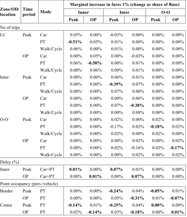
Table 10 Effects on demand, delay for car and occupancy in the buses from a 1 percent increase in fares, in inner versus outer zone and in the peak versus the off-peak
Zone/OD/ location
Time
period Mode
Marginal increase in fares 1% (change as share of Base)
Inner Inter O-O
Peak OP Peak OP Peak OP
No of trips
I-I Peak Car 0.05% 0.00% -0.03% 0.00% 0.00% 0.00%
PT -0.51% 0.05% 0.01% 0.00% 0.00% 0.00%
Walk/Cycle 0.06% 0.00% 0.01% 0.00% 0.00% 0.00%
OP Car 0.00% 0.05% 0.00% -0.03% 0.00% 0.00%
PT 0.06% -0.50% 0.00% 0.01% 0.00% 0.00%
Walk/Cycle 0.00% 0.06% 0.00% 0.01% 0.00% 0.00%
Inter Peak Car 0.00% 0.00% 0.06% 0.01% 0.00% 0.00%
PT 0.00% 0.00% -0.39% 0.07% 0.00% 0.00%
Walk/Cycle 0.00% 0.00% 0.07% 0.00% 0.00% 0.00%
OP Car 0.00% 0.00% 0.00% 0.06% 0.00% 0.00%
PT 0.00% 0.00% 0.07% -0.38% 0.00% 0.00%
Walk/Cycle 0.00% 0.00% 0.00% 0.08% 0.00% 0.00%
O-O Peak Car 0.00% 0.00% 0.02% 0.00% 0.02% 0.00%
PT 0.00% 0.00% -0.17% 0.02% -0.18% 0.02% Walk/Cycle 0.00% 0.00% 0.02% 0.00% 0.02% 0.00% OP Car 0.00% 0.00% 0.00% 0.02% 0.00% 0.02% PT 0.00% 0.00% 0.02% -0.16% 0.02% -0.17% Walk/Cycle 0.00% 0.00% 0.00% 0.02% 0.00% 0.02% Delay (%)
Inner Peak Car+PT 0.01% 0.00% 0.07% 0.01% 0.00% 0.00% OP Car+PT 0.00% 0.01% 0.00% 0.07% 0.00% 0.00% Point occupancy (pers./vehicle)
Border Peak PT 0.00% 0.00% -0.24% 0.04% -0.05% 0.01%
OP PT 0.00% 0.00% 0.05% -0.31% 0.01% -0.07%
Center Peak PT -0.14% 0.01% -0.25% 0.04% 0.00% 0.00%
OP PT 0.02% -0.14% 0.03% -0.18% 0.00% 0.01%
17 However, these elasticities are large compared to in to the supply elasticity of only 0,03 in Pyddoke et al.
Table 10 shows the effects on number of trips, congestion (in terms of delay) and crowding (in terms of occupancy) of differentiated marginal increases in fares. From Table 10, one can see that the effect on attractiveness of public transportation for the inner city is greater for changes in fares (elasticities about -0,50) than changes in supply. The reason for this is that for the inner city, trips are substantially shorter than for the O-O and Inter trips, which means that the generalized cost for I-I is much lower, which in turns means that the fare constitutes a larger share of the generalized costs. Supply changes, however, affect also inter and O-O trips (the effects on demand from supply adjustments is distributed over 2-3 OD-pairs).
The effect on crowding is larger for the fare changes on inter trips than for fare changes within zones. This stems from a combination of three factors. First and foremost, the inter trips are more in numbers in the baseline than for each of the other two categories. Second, they are much longer than the I-I trips; and third, the have higher elasticity than the O-O trips. Again, we can see that the effects on delays are modest. In Table 11, the financial outcomes of both marginal supply and fare adjustments are summarized.
Table 11 Financial outcomes for RPTA in SEK per week day from changes in subsidy level and capacity use of differentiated marginal (1%) increases in supply and fares. Figures are expressed as changes compared to baseline.
Adjusted quantity Supply Fare
Adjusted for
OD-pair Inner Outer Inner Inter O-O
Adjusted in period Peak OP Peak OP Peak OP Peak OP Peak OP
Fare revenue 222 458 232 504 214 287 1178 1604 222 311 Producer costs 1764 1940 3395 5404 18 9 97 51 -1 0 Producer surplus, without MCPF -1579 -1500 -3155 -4887 196 278 1092 1561 223 312 Change in subsidy* 0.05% 0.04% 0.11% 0.16% -0.02% -0.02% -0.09% -0.13% -0.02% -0.03% * In percentage points
Table 12 Social costs and benefits in SEK per week day of differentiated marginal (1%) increases in supply and fares
Adjusted quantity Supply Fare
Adjusted for OD-pair Inner Outer Inner Inter O-O
Adjusted in period Peak OP Peak OP Peak OP Peak OP Peak OP
Consumer surplus 235 865 862 1621 -407 -561 -1873 -2525 -299 -435 Producer surplus, without
MCPF -1542 -1482 -3164 -4900 196 278 1081 1554 223 312
Congestion benefits for
trucks -12 -10 2 3 -1 -1 -8 -7 0 0
Emissions benefits* -4 -3 -13 -10 0 0 1 1 1 1
Of which CO2 benefits** -1787 -1075 -3261 -4756 -154 -201 -474 -511 -8 -29 Net social benefits -116% -73% -103% -97% -79% -72% -44% -33% -4% -9% NSB as share of PS*** 235 865 862 1621 -407 -561 -1873 -2525 -299 -435 * Net benefits of emissions and taxation of emissions
***“NSB as share of PS” denotes net social costs as share of the absolute value of the producer surplus, and is a measure of the social return of public spending.
From Table 11, one can see that increases in supply in the outer zone is costly and the reduction in fares is much less so. In Table 12, the welfare effects of marginal supply and fare adjustments are summarized. From the calculations in Table 12, there appears to be an excess in both supply and fares in baseline (the only exception is fares for O-O in the peak). In some cases, this excess is large and the model suggests that there is socially beneficial to decrease supply as well as the fares in the inner zone and for the inter trips in the peak period (see the last row of Table 12). Somewhat surprisingly, the model suggest that it is most socially desirable to decrease supply in the inner zone during the peak. This is because frequency is highest, cost of supply is largest, and the model estimates large delays from congestion - and more buses on the streets worsen this situation. In the same time, crowding in vehicles is not a large problem on average in baseline, not even in the inner zone during peak hours.18
3.2.
Scenarios
In this section four different policy scenarios are analyzed (see eq. 37 in section 2.2). In the first scenario frequencies for each zone and time period are chosen to optimize welfare. In the second fares are chosen for each OD-pair and time period to optimize welfare. In the third fares and frequencies are chosen simultaneously to optimize welfare (without restrictions). Finally, in the Pareto scenario a further restriction is added, no consumer group (mode, period or zone) is allowed to have its welfare decreased.
Table 13 Policy parameter values in optima with different restrictions (as percent of baseline). Policy variable Fares only Supply only Welfare optimum Pareto scenario Supply level Inner, Peak 100% 60% 62% 64% Inner, OP 100% 74% 77% 76% Outer, Peak 100% 47% 51% 56% Outer, OP 100% 52% 54% 54% Fare level Inner, Peak 0% 100% 38% 38% Inner, OP 42% 100% 46% 46% Inter, Peak 38% 100% 44% 39% Inter, OP 52% 100% 48% 44% O-O, Peak 149% 100% 176% 43% O-O, OP 124% 100% 161% 0%
In line with Table 12, the estimates in Table 13 indicates that the optimal policy involves reductions in both fares (with two exceptions) and supply, and that for some relations these reductions are drastic, as for supply in the outer zone and for most of the fares. It can also be seen that optimal supply changes less between scenarios than do optimal fares, and that optimal fares depend more on supply than the other way around.
18 Note that the direction of trips has not been taken into account, and this could be an important limitation for
The optimal reductions in supply vary from 23 percent (in the inner city during OP in the Welfare optimum) to 53 percent (the outer zone during the peak in Supply only), and are generally larger in the outer zone than in the inner zone. In the inner zone, there are larger reductions for the peak than for the OP. In the two scenarios where fares are set without restrictions – Fare only and Welfare optimum – the fare level varies much with respect to OD-pair and less so with respect to time period. The level of optimal fares are similar for I-I and inter trips, where the model prescribes a more than 50% reduction. In stark contrast, for the O-O trips the model prescribes an increase of similar order. This is because in the inner zone, there is substantial external effects from car traffic in the form of congestion. I the other zone, such external effects do not exist but in fact there are slight positive external effects due to over taxation of car traffic.
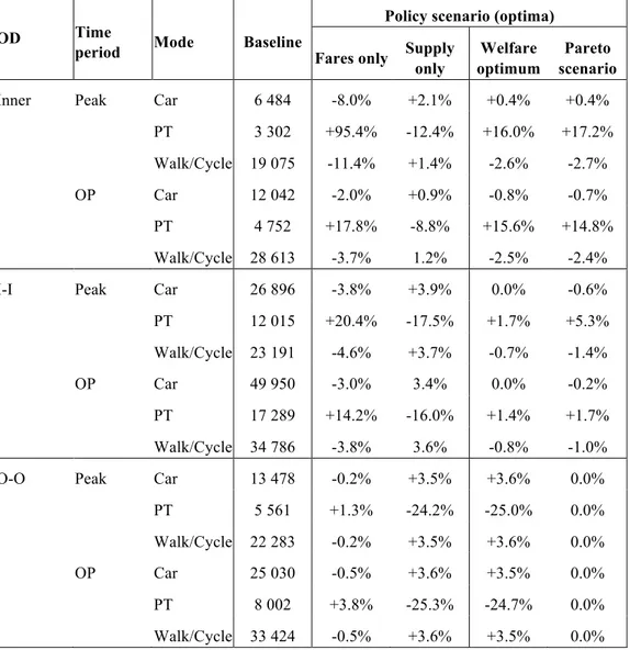
In Table 14 the effects in terms of demand for each mode, period and zone are shown.
Table 14 Changes in number of trips in the examined optima compared to baseline (in percent)
OD Time
period Mode Baseline
Policy scenario (optima)
Fares only Supply
only
Welfare optimum
Pareto scenario
Inner Peak Car 6 484 -8.0% +2.1% +0.4% +0.4%
PT 3 302 +95.4% -12.4% +16.0% +17.2%
Walk/Cycle 19 075 -11.4% +1.4% -2.6% -2.7%
OP Car 12 042 -2.0% +0.9% -0.8% -0.7%
PT 4 752 +17.8% -8.8% +15.6% +14.8%
Walk/Cycle 28 613 -3.7% 1.2% -2.5% -2.4%
I-I Peak Car 26 896 -3.8% +3.9% 0.0% -0.6%
PT 12 015 +20.4% -17.5% +1.7% +5.3%
Walk/Cycle 23 191 -4.6% +3.7% -0.7% -1.4%
OP Car 49 950 -3.0% 3.4% 0.0% -0.2%
PT 17 289 +14.2% -16.0% +1.4% +1.7%
Walk/Cycle 34 786 -3.8% 3.6% -0.8% -1.0%
O-O Peak Car 13 478 -0.2% +3.5% +3.6% 0.0%
PT 5 561 +1.3% -24.2% -25.0% 0.0% Walk/Cycle 22 283 -0.2% +3.5% +3.6% 0.0% OP Car 25 030 -0.5% +3.6% +3.5% 0.0% PT 8 002 +3.8% -25.3% -24.7% 0.0% Walk/Cycle 33 424 -0.5% +3.6% +3.5% 0.0%
The most important observations are the following. In the Welfare optimal scenario, public transport demand increases substantially for within inner zone trips, due to a larger reduction in fares than in frequency. However, outer-to-outer passengers experience both large reductions in supply and large increases in fares, and hence reduce their demand. The effect on total public transport demand is a small decrease (3 percent). In the Pareto scenario there are increases in public transport demand for the
inner zone, but without the drop in demand for the outer zone which means that total public transport demand increases (3 percent).
The effects on congestion (delay) and crowding (occupancy) from the switches in travel alternatives from Table 14, in combination with the supply changes in Table 13 are shown in Table 15.
Table 15 Delays and point occupancy in buses in baseline and in the examined optima respectively
Zone/
location Time period Mode Baseline
Policy scenario (optima)
Fares only Supply
only Welfare optimum Pareto scenario Delay
Inner Peak Car+PT 96% 89% 94% 89% 89%
OP Car+PT 42% 40% 42% 40% 40%
Point occupancy (pers./vehicle)
Border O* Peak PT 55% 60% 99% 100% 100% OP PT 42% 47% 66% 72% 79% Border I* Peak PT 55% 60% 78% 82% 88% OP PT 42% 47% 46% 50% 56% Center Peak PT 70% 98% 100% 119% 118% OP PT 54% 60% 66% 75% 74%
* Border O denotes the limiting occupancy at the border in the outer zone, while Border I denotes the limiting
occupancy at the border in the inner zone (remember that there is a kink at the border when supply in the two zones differs).
From Table 15, one can see that congestion is not much affected, while there are large effects on the occupancy in buses. In the outer zone, mean occupancy increases from less than 30 percent to around 30-50 percent for three of the scenarios (remember that mean occupancy in the outer zone is half of the point occupancy at the border). The effects on financial outcomes for the RPTA are shown in Table 16.
Table 16 Financial outcomes for RPTA in SEK per week day and changes in subsidy level and capacity use of different policy scenarios. Figures are expressed as changes compared to baseline.
Policy scenario Baseline Fares
only Supply only Welfare optimum Pareto scenario Fare revenue 572 515 -228 126 -101 859 -251 846 -339 206 Producer costs 1 232 885 -12 437 -558 273 -530 284 -509 228 Producer surplus, without MCPF -660 370 -215 689 +456 414 +278 437 +170 022
Subsidy level 54% +18% -23% +1% +14%
Capacity use in OP 67% +1% +9% +8% +3%
Optimizing welfare with fares imposes large costs to the RPTA in terms of revenue loss, counteracted by somewhat decreased costs due to shorter rotation times of vehicles due to reduced congestion.
There is, however, an interesting potential to optimize supply. The results indicate that this may reduce costs to almost half, suggesting a substantial current excess supply. In the scenarios where both fares and supply are chosen to optimize welfare, these savings are reduced a bit and the subsidy level is even increased (the positive absolute result is counteracted by the reduction in turn-over). The capacity use in OP is most affected in Supply only and Welfare optimum. Next, in Table 17, the implications in terms of total welfare are presented.
Table 17 Welfare social costs (negative sign) and benefits (positive sign) in SEK per week day of different policy scenarios. Figures are expressed as changes compared to baseline.
Policy scenario Baseline Fares only Supply only optimum Welfare scenario Pareto
Consumer surplus +324 052 -276 982 -23 589 +104 395
Producer surplus, without MCPF -660 370 -215 689 +456 414 +278 437 +170 022 Congestion benefits for trucks +1 147 +103 +1 027 +1 103
Emissions benefits -48 +1 574 +1 482 +1 087
Of which CO2 benefits +200 -282 -231 +559
Net social benefits (SEK) +44 755 +318 033 +340 888 +327 613
Three observations stand out. The first is that substantial improvements in social welfare can be gained by reducing supply in the Supply only scenario. The second is that optimization of Fares only does not achieve much compared to the Supply only scenario in terms of net welfare. And third, in the Pareto scenario social welfare can be improved without reducing generalized costs for any identified group (travelers with any mode, for any OD-pair, in any time period) in the model. This comes at a loss of social welfare compared to the welfare optimal scenario of 13 000 SEK/ week day, which is a rather small number compared to producer cost of 1 200 000 SEK/ week day in baseline (this difference may also be statistically non-significant when considering all sources of uncertainty in the analysis).
4. Discussion
A purpose of this study is to analyze fares and frequencies differentiated in time and space in Uppsala – a medium sized Swedish city – and to optimize them in different scenarios. The most important result of this study is that optimization of supply has larger potential to increase welfare than does optimization of fares. In fact, the total welfare is rather insensitive to fare changes, while these changes have large distributional effects, both between the producer and the consumers as a group, and among consumers. Therefore, a policy recommendation could be to base supply decisions on welfare
calculations, while leaving decisions about fares to elect politicians.
In the case of Uppsala, results indicate that a decrease of supply would increase welfare.19
Optimization in this respect would lead to substantial increases in occupancy rates, especially in the outer zone, where occupancy rates are low in the Baseline (only about 20-30 percent), and even more so if fares are decreased as in the welfare optimum and Pareto scenario. Of these two, the Pareto scenario may seem more attractive as most of the large total gains in the welfare optimum can be achieved without any consumer group (traveler by any mode, between any OD-pair, in any time period) being worse off in terms of generalized travel cost than in the Baseline. Also, in the Pareto scenario the total number of public transport trips, increase substantially (as well as there are some environmental benefits). We can see that from an environmental perspective it is more effective to decrease fares than to increase supply. This is because the fare reduction attracts travelers to the public transport mode and hence reduce the emissions from the cars, while not increasing the emissions from buses. Here there is obviously a tradeoff between crowding in buses and the environmental benefits that needs to be balanced, and we believe this tradeoff to be general.
Another point that we think is general is that we noticed that when policy is at an optimum, the model prescribes that an increase in supply should be accompanied with a decrease in fares. This is because an increase in supply means spare capacity that should optimally be utilized, so it is a welfare gain to increase the effort to attract consumers.
One interesting result relating to the work of Vickrey (1963) is that for the I-I and inter trips, the model in some cases prescribes lower fares in peak than in off-peak. We believe that this result is not general but emerges because cars trips in the inner zone are underpriced, which (in combination with inclusion of the MCPF) means that the model does not apply strict marginal cost pricing. Therefore, an interesting expansion of the present study is to examine what implication an optimization of parking fees would have on optimal public transport fares.
One obvious caveat with the fare system prescribed by the model is that the fares for inter zone trips are lower than for trips within the outer zone. The reason may be that for inter zone trips the car alternative is the most important mode, and these car trips end up in the city center where they contribute to increased congestion, which delays both public transportation and other car users. However, such a fare policy would not be practicable to implement, since it doesn’t make sense to pay more to travel one zone only than to travel two zones. Problems include acceptability of policy, distorted routing incentives and enforcement of policy. In future work such a restriction should be taken into account. However, because optimal supply is rather insensitive to fares, we don’t think the general recommendations would be much affected though.
At this stage, the model uses elasticities from Stockholm and is calibrated to somewhat coarse averages for occupancy. This carries the risk that local elasticities and occupancy rates may differ which in turn may influence the results. Results presented in e.g. Pyddoke et al. (2017) however point to similar indications of oversupply of services in Uppsala. In future work, it should be prioritized to
19 One interpretation of this could be that, because mean occupancy in the outer zone is as low as 20-30% in
baseline, an increase in demand does not by itself motivate a considerable increase in supply, which means that the Mohring effect in the outer zone is limited in baseline.