Data interpolation for groundwater
modelling
How choice of interpolation method and sample size affect the modelling
results
Frida Agerberg
Natural Resources Engineering, master's 2020
Luleå University of Technology
I
ACKNOWLEDGEMENTS
This report presents a thesis work within the Master Programme in Natural Resources Engi-neering at Luleå University of Technology. The thesis work covers 30 credits, corresponding to 20 weeks of full-time studies, and was conducted during the spring semester of 2020. The thesis work was performed in collaboration with Tyréns AB in Umeå.
I want to begin with a warm thank you to Jeffrey Lewis, external supervisor at Tyréns, whose expertise within the subject of geohydrology has been a valuable resource throughout the pro-ject. I also want to show my appreciation to the co-workers at Tyréns, especially within water and geotechnology, for making me feel welcome at Tyréns and for answering all my questions related to the thesis work. Finally, I direct a warm thank you to Jiechen Wu, supervisor at LTU, for your constructive input to the report and for your continuous kindness and support.
Umeå, May 2020 Frida Agerberg
II
ABSTRACT
Over the past several decades, the use of groundwater modelling has been increasing in order to better evaluate the complexities inherent in hydrogeological calculations. Information required for groundwater modelling is for example elevation of soil and bedrock layers, which often is collected by drilling. This is both time consuming and expensive, making it impossible to collect an unlimited number of data points. It is not uncommon that smaller hydrogeological investiga-tions are based on only three or four sample points. To approximate values of unknown points in the study area, the known values of the measured data is interpolated. The interpolation can be done with different methods, and the estimations of the elevation of geological layers at the unknown points might vary with different methods. How the uncertainty of the interpolations then affects the modelling results is generally unknown when simulating groundwater flow. The aim of the thesis work is to investigate how hydrogeological results from groundwater mod-els are affected by choice of interpolation method and by sample size of which the interpolation is based on. The hydrogeological models were simulated within the framework of a Swedish railway project where an unusually large number of probing data was available. The study focuses on two-dimensional, steady-state groundwater flow modelled in the software SEEP/W. Consequently, the objective of the modelling work was to simulate groundwater flow where the difference between the models was how the geometry of the geological layers was defined. The definition of the geometry was done with interpolations of the probing data with different interpolation methods and with interpolation based on different sample sizes. Twelve different interpolation methods in the software Surfer was used to interpolate the total of 357 data points. The interpolations that were estimated to be reliable were then used in the groundwater mod-elling. Groundwater models were also simulated based on a reduced amount of data in order to investigate the importance of sample size. The total amount of data points was reduced to 50%, 25%, 5% and 1% of the initial sample size before it was interpolated and then used to define the geometry in the groundwater models.
The study showed that although the choice of interpolation method and sample size affected the results of the modelled groundwater flow rate, none of the deviations between the model results were larger than what would be considered as acceptable in a hydrogeological context. The models based on at least 90 data points showed good precision while the precision of modelled groundwater flow decreased when sample size decreased. Thus, when interpolating data for groundwater modelling, the sample size should be determined by the required precision of the study. For the modelling of the 1% data, only one of the six models was possible to simulate. This since at least three data points are required for each geological layer in order to perform interpolations, and this was only obtained in one of six randomly selected data sets. The study indicates that around 10-20 sample points is a minimum for a study area with similar conditions as the reference project in order to have a high probability of obtaining enough data of all geo-logical layers of interest. Finally, the study indicates that there are other parameters in ground-water modelling, for example hydraulic conductivity and boundary conditions, that might have an equal of higher impact on the model results. These parameters should therefore also be de-termined with a high precision in order to gain accurate modelling results.
III
SAMMANFATTNING
Under de senaste årtiondena har användandet av grundvattenmodeller ökat för att bättre kunna hantera komplexitet inom hydrogeologiska beräkningar. För att kunna skapa en grundvatten-modell krävs exempelvis data över hur lager av jord och berg är beläget. Dessa geologiska data samlas vanligen i borrpunkter, vilket är både tidskrävande och dyrt. Detta gör det omöjligt att erhålla ett obegränsat antal mätpunkter och det är vanligt att mindre hydrogeologiska undersök-ningar endast utgår ifrån tre till fyra mätpunkter. Utifrån det begränsade antalet mätpunkter in-terpoleras kända nivåer av jord- och berglager för att approximera nivåer i okända punkter. Interpolering görs med hjälp av olika matematiska metoder och resultatet av dessa kan variera mellan olika metoder. Hur osäkerheter i interpolering sedan påverkar resultat från grundvatten-modellering är vanligtvis okänt.
Syftet med examensarbetet är att undersöka hur hydrogeologiska resultat från grundvattenmo-deller påverkas av val av interpolerings metod samt av antal mätpunkter som interpoleringen är baserad på. Grundvattenmodellerna skapades inom ramen av ett svenskt järnvägsprojekt där ovanligt stora mängder sonderingsdata fanns tillgängligt. Undersökningen fokuserar på steady-state grundvattenflöden i två dimensioner, modellerat i programmet SEEP/W.
Undersökningen utgick därmed från sonderingsdata i referensprojektet för att skapa ett antal grundvattenmodeller, där skillnaden mellan dessa var hur nivån av de geologiska lagren definie-rades. Detta gjordes med hjälp av olika interpoleringsmetoder och med interpolering baserad på olika mängder data punkter. Tolv olika interpoleringsmetoder i programmet Surfer användes för att interpolera de totalt 357 data punkterna. De interpoleringar som kunde antas vara rimliga användes sedan för att definiera geometrin i olika grundvattenmodeller. Grundvattenmodeller skapades även utifrån en reducerad mängd data för att undersöka betydelsen av antal mätpunkter vid interpolering. Antal mätpunkter reducerades till 50%, 25%, 5% och 1% och interpolering av dessa användes sedan för att definiera geometrin i olika grundvattenmodeller.
Studien visade att även om modeller baserade på olika interpoleringsmetoder och interpolering av olika antal mätpunkter genererade något olika resultat med avseende på modellerat grundvat-tenflöde, så var inget av resultaten mer avvikande än vad som i ett hydrogeologiskt sammanhang skulle klassas som acceptabelt. Vidare visade resultaten att modeller baserade på 90 data punkter eller mer hade en bra precision av modellerat grundvattenflöde samt att minskat antal mätpunkter ledde till minskad precision. Antal mätpunkter i en undersökning bör därmed väljas utifrån hur bra precision som bör uppnås. Dock kan ett lägre antal mätpunkter försvaras om erhållen precis-ion vägs mot hur resurskrävande insamling av data är. Modelleringen av 1% data visade att endast en av de sex modellerna gick att skapa. Detta var på grund av att minst tre datapunkter för varje geologiskt lager krävdes för att interpolera data och detta uppnåddes alltså bara i en av de slum-pade data seten. För att ha en hög sannolikhet att erhålla tillräckligt med data för varje jord- eller berglager av intresse indikerar denna studien på att 10 till 20 mätpunkter är tillräckligt i en under-sökning med liknande förutsättningar som i referensprojektet. Slutligen så indikerar studien på att det finns andra parametrar, exempelvis hydraulisk konduktivitet och randvillkor, som kan ha liknande eller större inverkan på modellerat grundvattenflöde och för att få noggranna resultat bör även dessa parametrar bestämmas med hög precision.
IV
TATBLE OF CONTENTS
1 INTRODUCTION ... 1 1.1 Background ... 1 1.2 Aim ... 2 2 THEORETICAL BACKGROUND ... 3 2.1 Groundwater flow ... 3 2.1.1 Hydraulic conductivity ... 42.2 Properties of soil and bedrock ... 5
2.2.1 Geotechnical investigations of hydraulic conductivity and soil stratigraphy ... 5
2.3 Groundwater modelling ... 6
2.3.1 Finite element method ... 6
2.4 Spatial data interpolation ... 7
2.4.1 Kriging ... 10
2.4.2 Radial basis function ... 10
2.4.3 Inverse distance weighting ... 11
2.4.4 Minimum curvature ... 11
2.4.5 Evaluating the accuracy of interpolation methods ... 11
2.4.6 Effect of sample size on data interpolations ... 12
2.4.7 Recent developments of interpolation methods ... 13
3 METHOD ... 14
3.1 Case study description ... 14
3.2 Overview of the approach ... 14
3.3 Primary processing of data ... 15
3.3.1 Generating data sets with reduced sample size ... 17
3.4 Data interpolation ... 18
3.5 Profile creation ... 19
V
3.6.1 Geometry ... 20
3.6.2 Material properties ... 20
3.6.3 Mesh settings ... 21
3.6.4 Calibration of boundary conditions ... 22
3.6.5 Interpretation of model results ... 22
4 RESULTS ... 24
4.1 Generated data sets ... 24
4.2 Interpolated contour maps ... 24
4.2.1 Altering interpolation method ... 25
4.2.2 Altering sample size ... 27
4.3 Modelled profiles ... 28
4.3.1 Altering interpolation method ... 29
4.3.2 Altering sample size ... 30
4.4 Calibrated total heads ... 31
4.4.1 Altering interpolation method ... 31
4.4.2 Altering sample size ... 31
4.5 Modelled groundwater flow rates ... 32
4.5.1 Altering interpolation method ... 32
4.5.2 Altering sample size ... 33
5 DISCUSSION ... 34
5.1 Altering interpolation method ... 34
5.2 Altering sample size ... 35
5.3 Suggestions for management ... 36
5.4 Limitations and uncertainties ... 37
5.5 Further work recommendation ... 37
6 CONCLUSIONS ... 39
VI
APPENDIX A – CONTOUR MAPS, ALTERING INTERPOLATION METHOD ... i APPENDIX B – CONTROUR MAPS, ALTERING SAMPLE SIZE ... iv APPENDIX C – GROUNDWATER MODELS ... vii
VII
NOTATIONS
Roman, upper case
{H} Vector of total head [m]
{Q} Vector of nodal flow [m3/s]
[K] Material properties matrix
A Cross-sectional area [m2]
K Hydraulic conductivity [m/s]
Q Groundwater flow [m3/s]
Roman, lower case
h Hydraulic head (total head) [m]
𝜕ℎ
𝜕𝑥 Hydraulic gradient [m/m]
t Time [s]
x Distance in horizontal direction [m]
y Distance in vertical direction [m]
z Elevation head [m]
ẑ0 Estimated value (elevation) at grid node 0 [m]
𝑧(𝑠𝑖) Value (elevation) at i-th measurement) [m]
Greek, upper case
Ψ Pressure head [m]
Greek, lower case
θ Volumetric water content []
VIII
LIST OF TABLES
Table 1: Soil classification according to grain size. ... 5
Table 2: Codes for termination of probing and description of the codes. ... 6
Table 3: List of the twelve interpolation methods in Surfer. ... 9
Table 4: Soil layers encountered in the probing data and the number of sample points they where encountered within.. ... 16
Table 5: Geological surfaces included in the initial data set and the number of sample points each material was encountered in. ... 17
Table 6: Amount of total data points for each sub sample percentage. ... 18
Table 7: Methods used for interpolation of the elevation data in the different data sets. ... 19
Table 8: Material properties settings in SEEP/W. ... 21
Table 9: Settings for hydraulic conductivity function and volumetric water content function for non-cohesive soil. ... 21
Table 10: Amount of data for each sub sample, geological surface and percent of data points from the total data set.. ... 24
Table 11: Evaluation of contour maps created by the twelve interpolation methods available in Surfer. ... 26
Table 12: Calculated sum of residuals for each geological surface and interpolation method. .. 27
Table 13: Groundwater levels used for model calibration. ... 31
Table 14: Boundary conditions stated in total head required to calibrate the models based on the four different interpolation methods. ... 31
Table 15: Boundary conditions stated in total head required to calibrate the models with sample size of 50%, 25%, 5% and 1%. ... 32
Table 16: Groundwater flow measured at x = 300 m in the models. ... 32
Table 17: Groundwater flow measured at x = 300 m for the models based on interpolations of 50%, 25%, 5% and 1% of the initial data set. ... 33
IX
LIST OF FIGURES
Figure 1: Illustration of the components of hydraulic head. ... 3
Figure 2: Illustrating the relationship between hydraulic conductivity and negative porewater pressure. ... 4
Figure 3: Schematic illustration of FEM. ... 7
Figure 4: Illustrating the concept of interpolating discrete data into a continuous surface. ... 8
Figure 5: Illustrating the principle of uncertainties when interpolating data regarding subsurface geology. ... 9
Figure 6: Overview of the study area.. ... 14
Figure 7: A typical vertical profile of the subsurface geology in the investigated area and definition of the geological surfaces. ... 17
Figure 8: The chosen profile line is shown in red. ... 19
Figure 9: Illustration of how the geometry was defined in SEEP/W. ... 20
Figure 10: Finite element mesh in SEEP/W. ... 22
Figure 11: Contour maps showing elevation of ground surface.. ... 25
Figure 12: Contour maps showing elevation of the bottom surface of the clay soil layer. ... 25
Figure 13: Contour maps showing elevation of bedrock surface.. ... 25
Figure 14: Contour maps showing elevation of ground surface.. ... 27
Figure 15: Contour maps showing elevation of the bottom surface of the clay soil layer. ... 28
Figure 16: Contour maps showing elevation of bedrock surface.. ... 28
Figure 17: Profile from model definition. ... 28
Figure 18: Modelled profiles of the simulated groundwater model Kriging 100%. ... 29
Figure 19: Modelled profiles of the simulated groundwater models from Kriging, Radial basis function, Inverse distance weighing and Minimum curvature interpolation. ... 30
Figure 20: Summary of modelled profiles of the simulated groundwater models based on reduced sample sizes. ... 30
1
1 INTRODUCTION
1.1 Background
Groundwater is defined as the water that completely fills the pore spaces in soil and the fractures in rock (Todd & Mays, 2005). Of all freshwater on earth, around 30% is available as groundwater (Nordström, 2005). Groundwater is an important source of drinking water in many parts of the world. Furthermore, the occurrence of groundwater affects geotechnical stability of soils as low-ering of groundwater table may cause subsidence (Sveriges geologiska undersökning, n.d.). Over the past several decades, the use of groundwater modelling has increased in order to better evaluate the complexities inherent in hydrogeological calculations. (Todd & Mays, 2005). Groundwater models are mathematical representations of water flow through porous media and are used to simulate parameters such as flow rates, porewater pressure distributions and flow paths (Kumar, 2015). Although groundwater models, by definition, are simplifications of a more com-plex reality they have proven useful in a variety of groundwater related engineering problems and for supporting decision making. There are numerous programs available for groundwater modelling (Todd & Mays, 2005). One that is commonly used in engineering work is SEEP/W (GEOSLOPE International Ltd, 2020).
Information required for groundwater modelling is for example elevation of soil and bedrock layers and groundwater level. This data is usually collected in a limited number of sample points, both due to practical and economical reasons (Lewis, personal communication, May 2020). Ge-ological data is often collected by drilling, which produces a single point of data. Drilling is also time consuming and expensive, making it impossible to collect an unlimited number of data points. In order to approximate values in unknown points, known values in measured sample points can be interpolated over the study area (Kitanidis, 1997). This is performed either by hand or with the use of mathematical methods. Kriging interpolation is one of the most commonly used interpolation methods in the fields of geology and hydrology (Li, Wan, & Shang, 2020), and is generally considered to produce good fitting surfaces for a variety of data sets (Kitanidis, 1997). Other examples of commonly used interpolation methods are Inverse distance weighting and Minimum curvature (Li & Heap, 2014). As each interpolation method has its own charac-teristics and level of complexity, results produced with different interpolation methods for the same data can differ from each other. In literature, interpolations are commonly evaluated ac-cording to how accurately the modelled data set fits to the measured data set (Li & Heap, 2014). However, no relevant research was found in the literature study within the thesis work regarding what impact the deviations among interpolated surfaces from different methods has on the results from groundwater models that they are imported into.
Regarding sample size, there are different rules of thumbs suggesting how many data points are needed to perform an accurate interpolation. A range of around 30 to 100 data points are sug-gested in different studies (Li & Heap, 2014). However, due to limited resources it is in practice common to use significantly smaller sample sizes (Li, Wan, & Shang, 2020). In small geohydro-logical projects it is common to only use around three of four sample points (Lewis, personal
2
communication, April 2020). In order to technically be able to perform an interpolation, most interpolation methods require a minimum of three datapoints (Golden Software LLC, 2019a). The framework of the thesis work is a large railway project commissioned by the Swedish Transport administration. The study area includes several major risk objects that may be severely impacted by the construction of the railroad due to the potential of subsidence. This area has therefore been studied with an unusual level of detail.
1.2 Aim
The aim of the thesis work is to investigate how hydrogeological results from groundwater mod-els are affected by choice of interpolation method and by sample size of which the interpolation is based on. The hydrogeological models were simulated within the framework of a Swedish railway project, which was chosen as a case study due to the heterogeneous geology of the investigated area and the unusually large amount of geotechnical data that was available within the project.
The following research questions were formulated to cover the aim of the thesis work:
• How does choice of method for interpolation of probing data affect the hydrogeological results gained from a groundwater model?
• How does sample size affect the hydrogeological results gained from a groundwater model?
The study focuses on two-dimensional, steady-state groundwater flow modelled in the GeoStu-dio software SEEP/W, which is commonly used in engineering.
3
2 THEORETICAL BACKGROUND
The following chapter aims to summarize the literature regarding the research topic. The theory works as a foundation for the choice of method as well as for the discussions and conclusions of this thesis work. To be able to simulate groundwater models, knowledge of groundwater flow, geology and concepts of geohydrological modelling are essential. Further, the theory of spatial data interpolation is a foundation of the thesis work.
2.1 Groundwater flow
Groundwater in a natural state is in constant movement, creating a flow which can be described by Darcy’s law, see equation 2.1-1 (Todd & Mays, 2005).
𝑄 = −𝐾𝐴𝜕ℎ
𝜕𝑥 (2.1-1)
Q [m3/s] is the groundwater flow, K [m/s] is the hydraulic conductivity, A [m2] is the
cross-sectional area and 𝜕ℎ
𝜕𝑥 [] is the hydraulic gradient (Todd & Mays, 2005). The negative sign
indi-cates that the groundwater flow is directed with the decreasing hydraulic head.
The hydraulic gradient is a measure of the rate of change in hydraulic head per unit length (Freeze & Cherry, 1979). Hydraulic head, also called total head, is the sum of the elevation head and the pressure head, see Figure 1 (Arthur & Saffer, n.d.). Groundwater flow is always directed from high to low hydraulic head (Todd & Mays, 2005).
Figure 1: Illustration of the components of hydraulic head (Arthur & Saffer, n.d.).
Two-dimensional groundwater flow can generally be described by a partial differential equation derived from Darcy´s law, see equation 2.1-2 (Todd & Mays, 2005).
𝜕 𝜕𝑥(𝐾𝑥 𝜕ℎ 𝜕𝑥) + 𝜕 𝜕𝑦(𝐾𝑦 𝜕ℎ 𝜕𝑦) + 𝑄 = 𝜕𝜃 𝜕𝑡 (2.1-2)
θ [] is the volumetric water content and t is time [s]. The equation states that the rate of change in the x direction of the hydraulic gradient times the hydraulic conductivity plus the rate of
4
change in the y direction of the hydraulic gradient times the hydraulic conductivity plus the flow at a boundary is equal to the change in volumetric water content over time (Todd & Mays, 2005). In a steady state condition, where the flow into the system is equal to the flow out from the system, there is no change in volumetric water content over time.
Both saturated and unsaturated groundwater flows can be calculated with Darcy’s law (Todd & Mays, 2005). However, an underlying assumption is that the flow is laminar. In most situations, this assumption is valid. It only becomes problematic where both the hydraulic conductivity and hydraulic gradient are unusually high.
2.1.1
Hydraulic conductivity
Hydraulic conductivity is defined as a measure of the ease with which water flows through a porous media (Jones & Mulholland, 2000). A variety of physical properties affects the hydraulic conductivity of a soil or rock (Todd & Mays, 2005). Porosity, particle size and shape of particles are some of the most important properties.
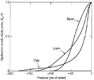
In the saturated zone, the hydraulic conductivity depends on the material properties, and is therefore constant if the material properties are homogenous (Todd & Mays, 2005). However, in case of unsaturated flow, the hydraulic conductivity is a function of the negative pressure head and volumetric water content. Furthermore, the volumetric water content is itself a function of negative pressure head during unsaturated conditions. The general shape of a hydraulic conduc-tivity function is shown in Figure 2.
Figure 2: Illustrating the relationship between hydraulic conductivity and negative porewater pressure (Todd & Mays, 2005).
As Figure 2 shows, the hydraulic conductivity decreases rapidly with the negative porewater pressure (Todd & Mays, 2005). The curve is steeper for coarser material and flatter for finer material such as clay soils. The flow of water through unsaturated soil is therefore much more complex than it is though saturated soil.
5
2.2 Properties of soil and bedrock
Soil is commonly classified by its composition according to grain size, see Table 1 (Todd & Mays, 2005). The composition has a major impact on the geotechnical and geohydrological properties of the soil (Svenska Geotekniska Föreningen, 2016).
Table 1: Soil classification according to grain size (Todd & Mays, 2005).
Material Particle size [mm]
Clay <0,004
Silt 0,004-0,062
Sand 0,062-2,0
Gravel 2,0-64,0
A rough classification of soil into cohesive soil and non-cohesive soil is commonly used in ge-otechnology as it is based on the strength of the soil (Svenska Geotekniska Föreningen, 2016). Non-cohesive soils are defined as the soils where the shear strength depends on friction between the soil particles while cohesive soils are those where the shear strength also depends on cohesion. Non-cohesive soils consists of granular material, including the sand and gravel fractions in Table 1 (Svenska Geotekniska Föreningen, 2016). Hydraulic conductivity in these soils is relatively high, generally above 1E-05 m/s. Saturated water content for non-cohesive soils is typically between 28% and 43%, but most commonly around 30% to 35% (Todd & Mays, 2005). In cohesive soils, clay is the major soil fraction (Svenska Geotekniska Föreningen, 2016). Its hy-draulic conductivity is relatively low, generally around 1e-09 m/s. Saturated water content for cohesive soils is typically around 40%, but can reach up to 50% (Todd & Mays, 2005).
Hydraulic conductivity for unfractured metamorphic and igneous rock is extremely variable and can range between 1e-06 to 1e-11 (Todd & Mays, 2005). Saturated water content for these rocks is limited to the fracture systems of the rock and is generally around 0% to 5% (Freeze & Cherry, 1979).
2.2.1
Geotechnical investigations of hydraulic conductivity and soil
stratig-raphy
In order to determine the hydraulic conductivity of a soil in field, a slug test is a common method to use (Svenska Geotekniska Föreningen, 2013). The test involves changing the groundwater level and then studying its recovery.
Investigation of soil stratigraphy can be performed with a method called probing (Svenska Geotekniska Föreningen, 2013). Probing is a group of geotechnical investigation methods where a steel cone is vertically driven into the ground while the effort of the process is recorded. There
6
are two commonly used methods. Weight sounding is more sensitive than other methods and is often used in lose to middle had soil types in order to determine the soil stratigraphy. In soil-rock sounding, the cone is usually driven at least 3 m into the soil-rock in order to determine where the bedrock starts. Type of probing termination is recorded according to the standard for all methods, see Table 2 (Svenska Geotekniska Föreningen and Byggnadsgeologiska Sällskapet, 2001).
Table 2: Codes for termination of probing and description of the codes (Svenska Geotekniska Föreningen and Byggnadsgeolo-giska Sällskapet, 2001).
Termination of probing, code Description
90 Sounding terminated without reaching refusal
91
The probe cannot be driven deeper down by normal procedure
92 Stop against stone or boulder
93* Stop against stone, bounder or bedrock
94* Stop against assumed bedrock
95*
Soil-rock probing. Drilling into assumed bed-rock.
*Code can be assumed to indicate stop against bedrock
2.3 Groundwater modelling
The attempt of a groundwater model is to create a mathematical representation of seepage through the subsurface geology in saturated and unsaturated conditions (GEOSLOPE International Ltd, 2020). Parameters such as flow rate, porewater pressure distribution, velocity and pathways can be modelled (GEOSLOPE International Ltd, 2015). Objectives for simulating a groundwater model can be to gain knowledge about a system’s behavior, to test cause and effect of various uncertainties and to identify additional data needed in order to increase the understanding of the system (Todd & Mays, 2005). Although the accuracy of groundwater mod-els tends to be uncertain, they are often the best representation available and are therefore widely used in engineering work and for supporting decision making.
The modelling software used in this thesis work is SEEP/W which is a modelling software com-monly used by engineers (GEOSLOPE International Ltd, 2020). The modelling software is based of finite element analysis (FEM).
2.3.1
Finite element method
Many physical processes in engineering are modelled by differential equations which are too complex to solve with classical mathematical methods (Ottosen & Pettersson, 1992). The issue of solving these differential equations can be addressed by a numerical method called finite ele-ment method (FEM). In FEM, general differential equations can be solved approximately with
7
dividing the investigated region into smaller parts, called finite elements, and then carrying out approximations over each element. When a solution is obtained for all the elements, these can be put together and an approximate solution for the entire body can be found, see Figure 3 (Ottosen & Pettersson, 1992).
Figure 3: Schematic illustration of FEM. The upper boxes shows how a physical phenomenon is approximated into a finite element equation and the lower boxes shows an example where a physical structure is approximated into finite elements (Ottosen & Pettersson, 1992).
In two-dimensional groundwater modelling, the partial differential equation to be solved is equa-tion 2.1-2 (GEOSLOPE Internaequa-tional Ltd, 2015). This differential equaequa-tion can be approxi-mated into the finite element equation bellow.
[𝐾]{𝐻} = {𝑄} (2.3.1-1)
[K] is a matrix that includes material properties and area of the element, {H} is a vector of total head and {Q} is a vector of nodal flow (GEOSLOPE International Ltd, 2015). The matrix [K], as well as either of the vectors {H} or {Q} must be specified in the model while the other vector is computed.
2.4 Spatial data interpolation
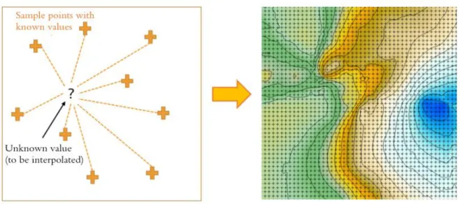
Due to the labor intensive nature of sampling and limited financial resources, data in geological investigations is collected at a limited number of sample points which are then used to represent the whole study area (Kitanidis, 1997). Interpolation means using the known values of the sample points in order to statistically estimate values at the unknown points. Thus, through interpolation it is possible to estimate a continuous surface of the values in the study area from an original discrete dataset of measurements, see Figure 4. This method can be applied to many different types of data and is a commonly used on geographical and geological data (GIS Resources, 2014a).
8
Figure 4: Illustrating the concept of interpolating discrete data into a continuous surface.
Methods for spatial interpolation is built upon Tobler’s first law of geography which states that everything is related to everything else, but that near things are more related than distant things (GIS Resources, 2014b). This principle is also called spatial correlation. In a hydrogeological example, spatial correlation would mean that it is more likely that the hydraulic conductivity at an unknown point is more similar to the hydraulic conductivity a sample point close by than to a sample point further away (Kitanidis, 1997).
Weighted average algorithms, built upon the principle of spatial correlation, is the foundation of most interpolation methods (Kitanidis, 1997). The linear estimator, see Equation 2.4-1, is a gen-eral formula for a weighted average algorithm.
ẑ0 = ∑𝑛𝑖=1𝜆𝑖𝑧(𝑠𝑖) (2.4-1)
ẑ0 is the estimated value at the unknown point, 𝑧(𝑠𝑖) is the measured value at the i-th location
and 𝜆𝑖 is the weight for 𝑧(𝑠𝑖) (Kitanidis, 1997). The weight (𝜆𝑖) represents the probability that
the value at the unknown point is equal to the value of the i-th measurement. The principle of
spatial correlation can be represented with higher weights for the measurement 𝑧(𝑠𝑖) closer to
the unknown point.
Uncertainties in spatial interpolation of subsurface geology is illustrated in Figure 5. The three lines shows three different suggestions of interpolating the elevation of the geological layers. Without further knowledge in a case like this it is impossible to know which interpolation is the best representation of the reality (Janakiraman, Masao, & Noboru, 2000).
9
Figure 5: Illustrating the principle of uncertainties when interpolating data regarding subsurface geology.
In this thesis work, the 3D mapping software Surfer (Golden Software LLC, 2019a), is used to perform the interpolations. There are twelve different interpolation methods available in Surfer, see Table 3, and the difference between them depends on how the weights in equation 2.4-1 are calculated and applied (Golden Software LLC, 2019a). For example, weights can either be calculated with a predetermined equation or estimated by minimizing the variance of the pre-diction errors (Li & Heap, 2014). For all interpolation methods in Surfer, a minimum or 3 datapoints are required to perform the interpolation (Golden Software LLC, 2019a).
Table 3: List of the twelve interpolation methods in Surfer.
Interpolation methods in Surfer
Inverse distance weighting Polynomial regression
Kriging Radial basis function
Minimum curvature Triangulation with linear interpolation
Modified shepard’s method Moving average
Natural neighbor Data metrics: Terrain slope
Nearest neighbor Local polynomial
In a study conducted by Yang et al. (2004), the twelve different interpolation methods available in Surfer were compared. The overall conclusion of the study was that there is no absolute best method and that optimal choice of interpolation depends on the situation. As a rule of thumb, the interpolation methods Kriging and Radial basis function produces relatively good represen-tations for smaller data sets (10 – 250 data points) but are slow for larger data sets (>1000 data points) (Golden Software LLC, 2019a). The method Minimum curvature produces good repre-sentations for large data sets and Inverse distance weighting works best for regularly spaced data. Yang et al. (2004) suggests reviewing the characteristics of the interpolation methods as well as the properties of the data set in order to select an optimal interpolation method. Furthermore, Yang et al. (2004) states that the results from the interpolation should be evaluated critically with the knowladge of the surface that is being interpolated.
10
In section 2.4.1 to 2.4.4, some of the more frequently used methods for interpolation are de-scribed.
2.4.1
Kriging
Kriging is one of the most commonly used interpolation methods in the field of geology and hydrology (Li, Wan, & Shang, 2020). It is generally considered to be one of the more flexible and accurate interpolation methods (Golden Software LLC, 2019a). Further, Kriging is consid-ered to produce good fitting surfaces for a variety of data sets (Kitanidis, 1997).
Kriging is an exact interpolator, which means that if a data point is located exactly at a grid node, the interpolated value should be equal to the known value of the data point (Kitanidis, 1997). The weights in equation 2.4-1 are determined according to minimum variance and to unbiasedness, where unbiasedness means that the sum of the weights must be equal to one. Kriging takes into account that datapoints located close to each other carries similar information with giving less weight to clustered data points. The flexibility of Kriging comes from that it, before performing the interpolation, also accounts for the spatial relationships between the meas-ured data points with variogram modelling. A variogram is used for fitting a function describing the spatial dependence of the variable to a plotted dependence of the measured data (Kitanidis, 1997).
One of the disadvantages to Kriging is that it can be slower for large data sets than other inter-polation methods (Golden Software LLC, 2019a).
2.4.2
Radial basis function
Radial basis function is a type of artificial neural network, which is a system intended to imitate the human brain in order to find implicit patterns within a data set (Rusu & Rusu, 2006). It is generally constructed with a three layers principle: an input layer, an output layer and a hidden layer which processes the input to something usable for the output layer. Arti-ficial neural networks are useful for recognizing patterns that are too complex for a human brain to recognize. As well as Kriging, Radial basis function is a flexible method which can be useful to interpolate most types of data sets. The interpolation method is an exact inter-polator and the precision of the interpolation is similar to Kriging but are considered slightly better for small data sets (Rusu & Rusu, 2006).
There are various types of Radial basis functions which uses different mathematical functions to define the optimal set of weights for the data points when interpolating a grid node (Golden Software LLC, n.d.). Thus, the different functions generate slightly different inter-polated surfaces. Among the group of Radial basis functions the Multiquadric function, which is the default in Surfer, is generally considered to generate good fitting surfaces for many of data sets.
11
2.4.3
Inverse distance weighting
Inverse distance weighting is one of the faster and more mathematically simple interpolation methods (Babak & Deutsch, 2009). The weights in the linear estimator are unbiased and calcu-lated by an equation where the value of the weights decreases exponentially with distance. A value of the exponent is manually select by the user and is commonly set to 2 (Babak & Deutsch, 2009), which is the default in Surfer (Golden Software LLC, 2019a). As the exponent increases, the weight decreases for the measures further away.
Inverse distance weighting is an exact interpolation method (Golden Software LLC, 2019a). The interpolation method is sensitive to characteristics such as to outliers and is prone to creating “bull’s eyes” around existing data points (Babak & Deutsch, 2009). Thus, Inverse distance weighting is more suitable for interpolating regularly spaced data than clustered data (Li & Heap, 2014)
2.4.4
Minimum curvature
Minimum curvature interpolation method attempts to generate the smoothest possible surface while aiming to pass through the measured data points (Golden Software LLC, 2019a). Mini-mum curvature is not an exact interpolator and the surface does not have to pass exactly through the data points. The interpolation is an iterative process where equations are applied over the grid until the successive changes are below a limit value or the maximum number of iterations is reached.
Minimum curvature interpolation works well for retaining small-scale features of the data (Li, Wan, & Shang, 2020).
2.4.5
Evaluating the accuracy of interpolation methods
Following steps are suggested by Golden Software (2019b) in order to evaluate which interpo-lation methods are suitable for a dataset.
1. Visual evaluation: Plot the interpolated data from all twelve interpolation methods into contour maps. The best representations of the original data are plots showing smooth contours and otherwise realistic shapes in relation to the interpolated physical property. The choice of interpolation method is narrowed down by eliminating the interpolation methods that can visually be assumed not to be good fits to the data.
2. Residuals: When it is not possible to visually determine which interpolation method suits the data best, grid residuals can be calculated to evaluate which interpolation is closest to the initial data set. The sum of the absolute value of the residuals for each interpolation can then be used to evaluate the remaining interpolation methods among each other.
12
The residual is the deviation between the observed data and the predicted value (Golden Software, LLC, 2019b). The interpolation method with the lowest sum of residuals can be as-sumed to be the best fit to the initial data set. An expression for sum of absolute value of residuals is shown in equation 2.4.5-1 (Kitanidis, 1997).
𝑆𝑢𝑚 𝑜𝑓 𝑟𝑒𝑠𝑖𝑑𝑢𝑎𝑙𝑠 = ∑|𝑧(𝑠𝑖) − ẑ𝑖| (2.4.5-1)
𝑧(𝑠𝑖) is the value at the i-th measurement and ẑ𝑖 is the estimated value at the same point (Kitanidis, 1997). In research, interpolation methods are commonly evaluated according how accurately the modelled data set fits to the measured data (Li & Heap, 2014) However, no rele-vant research was found in the literature study of this thesis work regarding what impact the difference among interpolated surfaces has on the results from groundwater models that they are imported into.
2.4.6
Effect of sample size on data interpolations
In a review of interpolation methods used in environmental science, Li and Heap (2014) states that that most interpolation methods produce similar results when the sample size is high. How-ever, when sample size is low, the choice of interpolation method has a significant impact on the resulting interpolated surfaces. The accuracy of interpolation methods is generally increasing with an increased sample size. The effects of sample size vary with interpolation methods as some require more data than others in order to obtain a satisfactory accuracy. Li and Heap (2014) furthermore suggests that there is a threshold where an increased sample size does not increase the accuracy of the interpolation significantly.
There is a variation of rules of thumb regarding sample size when interpolating data (Li & Heap, 2014). Webster and Oliver (2006) states that at least 100 data points are needed to produce a stable variogram, which is used in for example Kriging interpolation. Further Webster and Oliver states that 50 data points is an absolute minimum. However, sample sizes as low as 28 data points have also been proposed to perform an accurate interpolations (Li & Heap, 2014). Further, in a study of methods for interpolation of soil texture, it was concluded that a minimum of 80 was
needed for interpolation of spatial data in a study area of 11352 km2 (Li, Wan, & Shang, 2020).
In practice however, it is usual to have significantly lower sample sizes than stated above due to limited resources (Li, Wan, & Shang, 2020). Especially in smaller geohydrological projects it is not uncommon to only have around three or four data points to work with (Lewis, personal communication, April 2020).
Apart from sample size, the spacing of samples has an impact on the accuracy of the resulting interpolation (Li & Heap, 2014). Spacing of samples should be done with consideration of the scales of variation of the variable in the investigated area as too widely spaced samples are gen-erally found to significantly reduce the information in the interpolated maps (Li & Heap, 2014).
13
2.4.7
Recent developments of interpolation methods
During the last few decades, several methods of interpolation have been developed from the field of machine learning (Li & Heap, 2014). Although these methods are rarely used, Lin and Heap (2014) suggest that they might become more widely used in the future due to their high predic-tion accuracy. In research from Janakiraman et al. (2000) an interpolapredic-tion method called fuzzy-MLP neural network was developed and studied. It was evaluated in a geological context and judged to be more accurate than other comparasive interpolation methods. The method has the advantage, compared to the classical interpolation methods, of being based on some geolocical principles and being able to provide and indication of the reliability of the interpolation. Although these recently developed methods for interpolations are not studdied further in this thesis work, it can be useful to keep in mind that there are alternatives to the more classical interpolation methods.
14
3 METHOD
In the methods chapter, the approach followed in order to answer the research questions is described. Section 3.1 provides a description of the case study. Sections 3.2 to 3.6 explains the process of model simulation from primary processing of data to the final groundwater model.
3.1 Case study description
The framework of the study is a large railway project commissioned by the Swedish Transport administration. In a study area within this project, groundwater and geotechnical considerations were investigated carefully due to a concern that a lowered water table during and following construction may cause subsidence in the surrounding clay soils. The geology in the study area is heterogeneous which brings uncertainties regarding the groundwater flows. Due to the un-certainties, extensive geotechnical investigations have been performed leading to a relatively large amount of probing data available within the study area. The study area is approximately 1x1 kilometer and contains a total of 357 sample points, see Figure 6.
Figure 6: Overview of the study area. The black circles represent the sample points and the contour lines represents the topog-raphy.
3.2 Overview of the approach
As stated in section 1.2, the aim of the thesis work is to investigate how hydrogeological results from groundwater models are affected by choice of interpolation method and by sample size of which the interpolation is based on. To be able to investigate this, the probing data from the case study was used to simulate groundwater models with differences in how the geometry of the geological layers was defined. Different interpolation methods available in the software Surfer and interpolations based on different sample sizes were used to create vertical profiles of the
15
geological layers within the study area. These profiles were then imported into the modelling software SEEP/W where they defined the geometry of the geological layers within the model. One groundwater model was simulated based on each individual profile.
To logically explain the process of going from initial probing data to a simulated model, the work can be divided into the following four steps.
• Step 1 – Primary processing of data: The probing data from the geotechnical investiga-tions within the case study was used as input for the groundwater modelling. In this first step, geological materials to include in the groundwater models was chosen. This initial data set was then used to create several data sets with reduced sample sizes in order to simulate a lower availability of data. This was done using a method of random selection of data points in Excel.
• Step 2 – Data interpolation: The data sets generated in step one was interpolated in the software Surfer. The initial data set was interpolated using different interpolation methods available in the software. The data sets with reduced sample sizes were interpolated using Kriging interpolation method. The interpolations resulted in contour maps over the study area showing the elevation of the interpolated geological surfaces.
• Step 3 – Profile creation: From the contour maps of the geological surfaces created in step 2, two-dimensional profiles showing the elevation of the geological layers along a defined line in the study area were created. This was also done in the software Surfer. • Step 4 – Model simulation: Groundwater models were simulated in the software
SEEP/W. The profiles created in step 3 were used to define the geometry of the different geological layers, where one model was simulated based on each of the created profiles. Hydrogeological results from the models regarding groundwater flow rate was obtained. Total head required to calibrate the groundwater models was also noted.
The steps 1 – 4 are more toughly described in sections 3.3 to 3.6.
Parallel to the model simulation, a literature study was an ongoing process throughout the thesis work. The search engines Science Direct, Google Scholar and DiVA were used in order to gain knowledge and collect relevant information regarding the research topic. Also, user’s guides together with online tutorials for Surfer and SEEP/W were used to collect information about the software used in the thesis work and the theory that they are built upon. Textbooks in groundwater hydrology and geostatistics were also used in the literature study as a knowledge base of the subject.
3.3 Primary processing of data
Input data for the groundwater models was obtained from the geotechnical investigations of the case study. Different methods of probing had been performed, of which the most commonly
16
used were weight sounding and soil-rock sounding, described in section 2.2.1. Following infor-mation were extracted from the total of 357 points of probing data in order to define the eleva-tion of the geological layers and the elevaeleva-tion of the groundwater table in the study area:
• Elevation of ground surface. Found in all of the 357 sample points. • Elevation of bedrock surface. Found in 131 of the sample points.
• Elevation of the bottom surface of soil layers. See Table 4 for a list of soil layers encoun-tered in the probing data and in how many of the sample points they where found. • Codes for termination of probing, labeled according to the Swedish notation system, see
Table 2.
• Groundwater levels measured in 16 groundwater wells. 1 to 53 measurements in each well had been taken over a time period of 2 years.
• Hydraulic conductivity of the non-cohesive soil layer. Determined with a slug-test.
Table 4: Soil layers encountered in the probing data and the number of sample points they where encountered within. Total number of sample points was 357.
Soil layers Number of sample points
Non-cohesive soil 265 Clay soil 256 Unknown material 62 Filling 43 Blocks 21 Till 7 Peat 6 Silt 5
The data above was further processed in order to generate an initial data set on which to base the modelling work. In order not to make a more complex model than necessary, only the geological material encountered in a relatively large amount of the probing data were used to model the system. Furthermore, extension of the bedrock data could be done as some data of the bottom of the non-cohesive soil layer could be assumed to be equivalent to the surface of the bedrock. This assumption was made as the non-cohesive soil, in most data points, was the deepest located soil layer, see Figure 7. The codes of termination of probing was used to find in which data points the non-cohesive soil data could be added to the bedrock surface data. For stop codes 93, 94 and 95, assumptions were made that the bottom of the non-cohesive soil was equal to the bedrock surface as the stop code indicated the encounter of bedrock, see Table 2.
17
Figure 7: A typical vertical profile of the subsurface geology in the investigated area and definition of the geological surfaces.
Thus, selection of which geological data to include in combination with an extension of the bedrock data resulted in the initial data set showed in Table 5.
Table 5: Geological surfaces included in the initial data set and the number of sample points each material was encountered in.
Geological surface Number of sample points
Ground surface 357
Bottom surface of clay soil layer* 256
Bedrock surface (extended with bottom surface of non-cohesive
soil layer) 200
* Written as “Clay soil” further in the report.
In addition to the elevation of the geological layers, the data from the groundwater wells was used for simulation of the groundwater models. For the wells with several measures of ground-water level, the mean value was used for defining the groundground-water level in the models.
3.3.1
Generating data sets with reduced sample size
In order to simulate a lower availability of data, sub samples with reduced sample sizes were created. This was performed in Excel, where all data points in the initial data set first were randomly sorted and then the top 50%, 25%, 5% and 1% of the rows were selected. This oper-ation was performed 6 times in order to get 6 different data sets for each required percent of the initial data. Thus, 24 new individual data sets were created, each containing elevation data of ground surface, clay soil and bedrock surface, see Table 6.
18
Table 6: Amount of total data points for each sub sample percentage.
Sub sample [% ] Total amount of data points
100% (1 data set) 357
50% (6 data sets) 180
25% (6 data sets) 90
5% (6 data sets) 18
1% (6 data sets) 4
As the information of the elevation of ground surface existed in all probing data, the number of data points of ground surface was equal to the total amount of data points in Table 6. However, for clay soil and bedrock surface, the amount of data points was less than in Table 6 as information of the material did not exist in all data points. For a more detailed description of the reduced data sets, see section 4.1 in the results chapter.
3.4 Data interpolation
The software Surfer was used to interpolate the elevation data of each geological surface in the initial data set and in the reduced data sets. Surfer is a 2D and 3D mapping, modelling and analyzing software, often used for interpolation of data (Golden Software LLC, 2019a).
The initial data set, containing the total amount of data points, was interpolated with each of the twelve available interpolation methods in Surfer, see Table 7. This was done to be able to com-pare how the results from the groundwater models differ when using different relevant interpo-lation methods. When evaluating the interpointerpo-lation methods, the contour maps were evaluated according, credibility of geological properties, smoothness of the contour lines and sum of re-siduals, as suggested in section 2.4.5. The interpolation methods whose contour maps were eval-uated to be representative were further used for defining the geometry of the geological layers in the groundwater models while the rest of the interpolations where sorted out.
Kriging interpolation method was used to interpolate the data sets of 50%, 25%, 5% and 1% of the total amount of data, see Table 7. As the aim with these interpolations were to compare how the sample size affects results in hydrogeological modelling, only one interpolation method was used. Kriging interpolation method was chosen as it, as mentioned in section 2.4.1, is commonly used the field of hydrogeology and often is recommended as it is considered to created good representations for most data sets. For the same reason, Kriging interpolation method was also used to interpolate the mean groundwater levels in the study area.
19
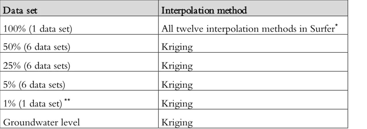
Table 7: Methods used for interpolation of the elevation data in the different data sets.
Data set Interpolation method
100% (1 data set) All twelve interpolation methods in Surfer*
50% (6 data sets) Kriging
25% (6 data sets) Kriging
5% (6 data sets) Kriging
1% (1 data set) ** Kriging
Groundwater level Kriging
*For a list of all interpolation methods in Surfer, see Table 3.
**Only one of the sic data set of the 1% data was possible to interpolate in Surfer due to limited amount of data for some of the geological layers.
For each data interpolation, a contour map was created showing the elevation of the geological surface. Due to the limited amount of data points in the 1% data sets, interpolation was only possible to perform for one of the six generated data sets.
3.5 Profile creation
The contour maps for the three geological surfaces were combined into one map for each set of interpolated surfaces. From these overlaid maps, two-dimensional vertical profiles were created showing the elevation of the geological layers along the profile line defined in Figure 8.
Figure 8: The chosen profile line is shown in red. Kriging 100% ground surface contour map in the background.
The profile line was chosen with the aim of finding a cross-section in the study area with the potential of producing a maximum difference between the simulated groundwater models. Thus, a section which had a continuous non-cohesive soil layer for some of the interpolation methods but not for others was searched for. This was considered to represent a largest deviation between 2D groundwater models as flow will be restricted when there is a non-continuous non-cohesive soil layer.
20
Following profiles were created along the chosen profile line:
• Profiles for the 100% data set: one profile for each interpolation method whose contour maps had been evaluated to be representative.
• Profiles for the 6 different 50% data sets. • Profiles for the 6 different 25% data sets. • Profiles for the 6 different 5% data sets.
• One profile for the data set of 1% that was possible to interpolate. • One profile for the interpolated mean groundwater level.
3.6 Model simulation
The groundwater models were simulated in SEEP/W, a software that preforms finite element analyses of groundwater flow in saturated/unsaturated porous media (GEOSLOPE International Ltd, 2020). Two-dimensional steady-state groundwater flow was modelled.
Section 3.6.1 describes the geometry definition of the groundwater models. One model was simulated for each different definition of input geometry. The following settings described in sections 3.6.2 were identical for all models. The input boundary conditions, described in section 3.6.4, were defined through model calibration.
3.6.1
Geometry
The profiles created in Surfer were imported into SEEP/W to define the geometry of the geo-logical layers clay soil, non-cohesive soil and bedrock. The geometry of the geogeo-logical layers was linearly extended in the x direction in order to prevent the boundary conditions from dictating the groundwater levels in the study area. The geometry within the red square in Figure 9 was generated from the Surfer profile and the geometry outside the square was extended linearly from the edges of the profile.
Figure 9: Illustration of how the geometry was defined in SEEP/W. The geometry within the red square was generated from the Surfer profile and the geometry outside the square was extended linearly from the edges of the profile.
3.6.2
Material properties
The settings in Table 8 were made for the geological materials in the groundwater models. The material settings were identical for all the simulated models.
21
The values of the hydraulic conductivities and saturated water contents were set according to the suggestions from Jeffrey Lewis (personal communication, Mars 2020). The exception was the hydraulic conductivity of the non-cohesive soil which instead had been measured in field with a slug-test during the geotechnical investigations.
Table 8: Material properties settings in SEEP/W.
Geological layer Ksat [m/s] Saturated water content [] Material model
Clay soil 1e-09 0,4 Saturated flow only
Non-cohesive soil 7e-07* 0,35 Saturated/unsaturated flow
Bedrock 1e-08 0,05 Saturated flow only
* Measured in field with slug-test.
Groundwater flow in the clay soil layer and in the bedrock were set to be saturated only. How-ever, the groundwater flow in the non-cohesive soil layer was set to saturated/unsaturated. This setting was made in order to allow for a decrease in hydraulic conductivity in the non-cohesive soil when the layer was situated above modelled phreatic surface, see section 2.1.1, and thus providing more exact calculations. This was done as most of the groundwater flow was expected to occur in the non-cohesive soil.
The settings of hydraulic conductivity function and volumetric water content function in Table 9 were applied to the non-cohesive soil as they are required for calculations of saturated/unsatu-rated groundwater flow. The specific functions for hydraulic conductivity and volumetric water content were chosen after suggestions from Jeffrey Lewis ((personal communication, Mars 2020)
Table 9: Settings for hydraulic conductivity function and volumetric water content function for non-cohesive soil.
Geological layer Hydraulic conductivity function Volumetric water content function
Non-cohesive soil Fredlund-Xing-Huang Sample function: Silty sand
3.6.3
Mesh settings
The global element size was set to 10 meters, which means that the sides of the finite elements in the model were approximately 10 meters. This was done with respect to the speed of the calculations versus the precision of the calculations. Furthermore, when comparing model results from a model with a smaller element size no significant differences in model results were seen which was why the element size of 10 meters was considered sufficient.
The size of the mesh within the non-cohesive soil layer, was set to a ratio of 0,1 of the global element size in order to preform more precise calculations in this layer, see Figure 10.
22
Figure 10: Finite element mesh in SEEP/W. The global element size in the clay soil and in the bedrock is set to 10 meters. The global element size in the non-cohesive soil is set to 1 meter.
3.6.4
Calibration of boundary conditions
Calibration of the groundwater models were performed regarding the boundary conditions. Boundary conditions were defined at the endpoints of the models as total head. This was done in order to be able to calculate the groundwater flow within the model, as suggested in section 2.3. The total head at the boundaries (x=-500 m and x=1600 m) were calibrated so that the modelled groundwater lever would match the generated profile of the mean groundwater level in the study area. The aim of the calibration was to match the groundwater level within ± 1 m at three points evenly spread out along the profile (x=0 m, x=450 m and x=900 m). In a hy-drogeological context this is a relatively exact calibration (Lewis, personal communication, May 2020).
For some of the simulated groundwater models, this accuracy of calibration was not possible. In that case only the two points at the edges (x=0 m and x=900 m) where used for calibration and it was noted that the complete calibration was not possible to perform.
3.6.5
Interpretation of model results
Groundwater flow rate through the model at the cross-section x = 300 m was obtained from all simulated models. An element thickness of 1 m was considered for the cross section. The mod-elled flow rates were compared in order to analyze how the different interpolations of the geo-logical data affected the groundwater models.
Furthermore, the calibrated total heads at the model boundary were also noted. Failure in cali-brating the groundwater levels in all three points or unrealistic values of hydraulic head indicated that the model was less likely to be accurate. A successful calibration indicated a more reliable groundwater model.
There were in this study no means of measuring the actual groundwater flow in field. Therefore, the accuracy of the modelled groundwater flow rates could not be compared with a known
23
value. Instead, the Kriging model based on 100% of the data was used as a reference for com-paring the modelled flow rates among the different simulated models. The interpolation method Kriging was used as it is commonly recommended for interpolating hydrogeological data.
24
4 RESULTS
In this chapter, the results from the thesis work are presented. Section 4.1 shows a summary of the generated data sets with reduced sample sizes. Section 4.2 shows results of the interpolated contour maps and the calculated sum of residuals. Section 4.3 provides a description of the geo-logical profiles in the simulated groundwater models. Section 4.4 shows the results regarding the calibrated total heads and section 4.5 shows the modelled groundwater flow rates from the sim-ulated models.
4.1 Generated data sets
After reducing the sample sizes with random selections of data points, the data sets summarized in Table 10 were generated. As the information of the elevation of ground surface was found in all the sample points, the reduced data sets have the same amount of data points of ground surface in all sub samples. For clay soil and bedrock surface on the other hand, the amount of data points varies between different sub samples as information about these layers did not exist in all sample points.
For the data sets of 1%, there were only one random selection that generated a sub sample where three or more data points were available for each geological surface. As three data points are required to perform interpolations in Surfer, see section 2.4, only sub sample number 5 included enough information for creating groundwater models.
Table 10: Amount of data for each sub sample, geological surface and percent of data points from the total data set. Selection number 0 represents the initial dataset with 100% of data points.
Sub sample Ground surface Clay soil Bedrock surface
0 (100% ) 357 256 200 50% 25% 5% 1% 50% 25% 5% 1% 50% 25% 5% 1% 1 180 90 18 4 128 62 14 1* 92 45 13 3 2 180 90 18 4 122 57 8 1* 105 56 12 3 3 180 90 18 4 128 68 13 3 105 53 11 2* 4 180 90 18 4 127 62 15 3 97 54 12 2* 5 180 90 18 4 129 61 12 3 101 48 11 3 6 180 90 18 4 133 67 13 4 99 49 9 2*
*Not enough data points to perform an interpolation.
4.2 Interpolated contour maps
Interpolations of all data sets were performed in order to create continuous surfaces of the data within the study area. Section 4.2.1 presents the interpolations of 100% of the initial data based on different interpolation methods and section 4.2.2 presents interpolations of the reduced data sets with Kriging interpolation method.
25
4.2.1
Altering interpolation method
The initial data set, containing 100% of the sample points, was interpolated with each of the twelve interpolation methods in Surfer. The interpolation of the elevation data of each material generated continuous surfaces in the shape of contour maps. The contour maps show the eleva-tion of the geological surface in the study area, where points with the same elevaeleva-tion are con-nected with contour lines. Figure 11 shows the four different interpolations of ground surface that where evaluated to be the most representative of the twelve performed interpolations, see Table 11. Figure 12 shows the same four interpolation methods, but for clay soil, and Figure 13 shows the four interpolations for bedrock surface. For a compilation of all contour maps created for each geological surface, see Appendix A.
Figure 11: Contour maps showing elevation of ground surface. Created from the interpolation methods Kriging, Radial basis function, Inverse distance and Minimum curvature.
Figure 12: Contour maps showing elevation of the bottom surface of the clay soil layer. Created from the interpolation methods Kriging, Radial basis function, Inverse distance and Minimum curvature.
Figure 13: Contour maps showing elevation of bedrock surface. Created from the interpolation methods Kriging, Radial basis function, Inverse distance and Minimum curvature.
26
All interpolations were evaluated visually according smoothness of contour lines and otherwise geologically realistic shapes, see 2.4.5. The interpolation methods Kriging, Radial basis function, Inverse distance and Minimum curvature could after visual examination be assumed more accu-rate than the other eight interpolations, see Table 11. The eight interpolation methods that where evaluated as less representative, either due to sharp edges in the contour line or otherwise unrealistic shapes according to geology, were sorted out.
Table 11: Evaluation of contour maps created by the twelve interpolation methods available in Surfer.
Interpolation method Comment
B es t re pre se nt at io
ns Inverse distance weighting Smooth surface and realistic shape
Kriging Smooth surface and realistic shape
Minimum curvature Smooth surface and realistic shape
Radial Basis Function Smooth surface and realistic shape
E va lu at ed le ss re pre se nt ati ve
Natural neighbor Sharp edges
Triangulation with linear
interpola-tion Sharp edges
Modified Shepard’s method
Unrealistic shape due to contour lines that ends in the middle of the plot
Nearest neighbor Sharp edges
Polynomial regression Unrealistic shape due to linear surface
Moving average
Unrealistic shape due to arc-shaped contours
Data metrics: terrain slope Unrealistic shape, scattered dots
Local polynomial Sharp edges
The interpolations in Table 11 that were visually evaluated to be representative were further evaluated according to sum of residuals, see section 2.4.5. The calculated sum of residuals for each interpolation is presented in Table 12. Table 12 shows that Radial basis function has the lowest sum of residuals throughout all layers, which is an indication that this interpolation is a slightly better representation of the initial data points than the other interpolations. Kriging and Minimum curvature have relatively similar sums of residuals. The calculated sum of residuals for Inverse distance weighting are higher than the other compared interpolation methods, which indicates that the representation is less reliable.