Софийски университет „Св. Климент Охридски”
Факултет по Математика и Информатика
Катедра „Софтуерни технологии”
Специалност „Информатика”
Специализация „Софтуерни технологии”
ДИПЛОМНА РАБОТА
Тема:
Интегриране на методи за формален анализ
в Progress IDE
Дипломант: Динко Панчев Иванов, Ф№ М22541 Научен ръководител: доц. Силвия Илиева, катедра „Софтуерни технологии”, ФМИ Консултант: Анета Вулгаракис, университет „Малардален”, Швеция2
Master of Science Thesis
Dinko Panchev Ivanov
Integrating formal analysis methods in
PROGRESS IDE
Mälardalen Research and Technology Centre
Thesis supervisor: Aneta Vulgarakis
Thesis examiner: Cristina Seceleanu
{
aneta.vulgarakis
,
cristina.seceleanu}@mdh.se
3 Abstract
In this thesis we contribute to the Progress IDE, an integrated development enviroment for real-time embedded systems and more precisely to the REMES toolchain, a set of tools to enabling construction and analysis of embedded system behavior models. The contribution aims to facilitate the formal analysis of behavioral models, so that certain extra-functional properties might be verified during early stages of development. Previous work in the field proposes use of the Priced Timed Automata framework for verification of such properties. The thesis outlines the main points where the current toolchain should be extended in order to allow formal analysis of modeled components. Result of the work is a prototype, which minimizes the manual efforts of system designer by model to model transformations and provides seamless integration with existing tools for formal analysis.
4 Table of Contents
1 Introduction………...7
1.1 Goals……….8
1.2 Structure of the thesis………9
2 Background………..10
2.1 Theoretical Background………. 10
2.1.1 ProCom component model………10
2.1.2 REMES………11
2.1.3 Timed Automata………...12
2.1.4 Priced Timed Automata………13
2.2 Technological Background……… 15
2.2.1 UPPAAL………..15
2.2.2 Eclipse……… 16
2.2.3 Eclipse Launching Framework………18
2.2.4 Eclipse Modeling Framework………19
2.2.5 Graphical Modeling Framework……….19
2.2.6 Object Constraint Language………...21
2.2.7 Atlas Transformation Language……….………21
2.2.8 Query-View-Transformation……….………23
2.2.9 REMES GUI……….………23
2.2.10 UPPAAL Modeling tools……….……….24
2.2.11 Attribute Framework……….………26
3 Problem Analysis……….……….27
3.1 Integration between ProCom and REMES……….………. 28
3.2 REMES GUI Extension……….……….29
3.3 PTA Transformation……….………..30
3.4 UPPAAL Integration……….………31
4 Solution Design……….……….32
4.1 Integration between ProCom and REMES……….………32
4.2 REMES GUI extensions……….………34
4.2.1 Definition of constants, variables and resources………….…………35
4.2.2 Introduction of Control Points……….…………38
4.3 PTA transformation……….43
4.3.1 Reflecting ProSave components communication in PTA…………43
4.3.2 Reflecting ProSys components communication in PTA………45
4.3.3 Translating Clocks into PTA………48
4.4 UPPAAL integration………..50
4.4.1 UPPAAL API……….50
4.4.2 Engine connection and lifecycle……….51
4.4.3 Model………52
4.4.4 UPPAAL perspective……….53
4.4.5 UPPAAL Simulator……….53
4.4.6 UPPAAL Variables………. 54
4.4.7 Graphical Simulation Trace………..54
4.4.8 Console View……….56
4.4.9 UPPAAL Simulator launch configuration……….56
5
4.4.11 UPPAAL Preference page………58
4.4.12 Context help………59
4.4.13 Logging………59
5 Prototype Description……….60
5.1 Integration between ProCom and REMES……….60
5.2 REMES GUI extensions……….60
5.3 PTA Transformation……….63
5.4 UPPAAL integration………..64
5.4.1 Configuring the UPPAAL plugin………64
5.4.2 Run the simulator ……….65
5.4.3 Run the verifier……….………67
6 Conclusion………71
7 References………..73
Appendix A - UPPAAL Engine API……….75
6 List of Figures and Tables
Figure 2-1 ProSys Subsystem………..10
Figure 2-2 ProSave Component………..11
Figure 2-3 REMES Composite Mode……….12
Figure 2-4 Lamp-User Timed Automata………13
Figure 2-5 Lamp-User Timed Automata extended with cost………14
Figure 2-6 Eclipse Platform Overview……….17
Figure 2-7 GMF Dashboard……….20
Figure 3-1 User workflow diagram………27
Figure 3-2 ProSys port to REMES variable mapping example………28
Figure 3-3 Sample ProCom project structure……….33
Figure 4-1 Referable entities in REMES metamodel ……….35
Figure 4-2 Compartment mappings in the GMF mapping model………36
Figure 4-3 Definition of compartments in the properties view……….37
Figure 4-4 Definition of in-place editing for constants………37
Figure 4-5 Control point entities in the REMES metamodel………38
Figure 4-6 Control points legend………..39
Figure 4-7 Example of invalid connection in REMES diagram………41
Figure 4-8 ProSave component communication example……….43
Figure 4-9 PTA template for C1 component……….44
Figure 4-10 PTA template for C2 component……….44
Figure 4-11 ProSys component communication example……….46
Figure 4-12 Generated PTA template for message channel………..46
Figure 4-13 PTA template for C2 ProSys component………47
Figure 4-14 Non-lazy mode synchronizer template ………..47
Figure 4-15 Example of ProSys component with Clock………48
Figure 4-16 PTA template for Clock……….49
Figure 4-17 PTA template for component connected with clock……….49
Figure 4-18 UML diagram of the UPPAAL model………..51
Figure 4-19 UML diagram of the UPPAAL model wrapper layer………53
Figure 4-20 UML diagram of UPPAAL engine options………58
Figure 5-1 Creating new behavior attribute……….60
Figure 5-2 Screenshot of the extended REMES diagram editor………..61
Figure 5-3 ProCom project structure after transformation……….63
Figure 5-4 UPPAAL plugin preference page……….64
Figure 5-5 UPPAAL simulator configuration dialog………65
Figure 5-6 UPPAAL perspective in action………..66
Figure 5-7 UPPAAL verifier configuration dialog – main tab………..67
Figure 5-8 UPPAAL verifier configuration dialog – queries tab……….68
Figure 5-9 UPPAAL verifier configuration dialog – options tab………....69
7
1 Introduction
Modern embedded systems pose high requirements to the Component Based Software Engineering (CBSE). Embedded systems have specific needs, which are imposed of the limited resources (CPU, memory) and the mission critical tasks, which the embedded system should perform. This leads to a specific aspect in the development, which is that certain properties of the systems should be evaluated at very early design stage of a component or system. For example during the architectural design of a system targeted to the vehicular domain, the designer should be able to estimate whether the current architecture satisfies certain properties, such as liveliness and whether the developed components fit within the resource profile of the target platform (vehicle). At some later stage of the development cycle, there might be a need to replace a component for some reason. Then a tradeoff analysis should be performed.
Those problems might be categorized in two main categories. A framework/component model for embedded system development should provide:
1. A way to define resource consumption and timing of a component and its resource-wise behavior at all stages of the development. 2. Methodology and tools for analysis of the timing and resource
behavior of the components.
ProCom [1] is a component model intended for design of embedded systems. It has been developed as part of PROGRESS, which is a large research project sponsored by the Swedish Foundation for Strategic Research.
To solve the first category problems, ProCom is backed by the REMES behavior modeling language [2][3]. REMES is not tightly coupled to ProCom, but provides generic framework for defining how a component consumes various resources (CPU, memory, bandwidth, etc.). REMES provides also a way to describe the internal states of a component and their behavior in time aspect. To tackle the problems in the second category, REMES needs the proper methodology for analysis. Since REMES is a time-state based modeling language, it could easily be mapped to the domain of priced timed automata and thus the resource analysis
8
problems could be formalized in the corresponding framework. This is where the scope of the current thesis falls into. The main goal of the thesis is to:
Integrate formal analysis techniques in the Progress IDE. The provided solution should allow the system designer to assign a REMES behavior model to a ProCom component and to perform formal analysis and verification of certain properties using the priced timed automata theory.
Progress IDE is an integrated development environment for component-based real-time embedded systems. It integrates a set of tools and frameworks to provide engineering support for the whole development process. The environment enables pure component-based development - main development units are the ProCom components and low-level artifacts are derived via automated code synthesis or generation of code skeletons. Progress IDE provides a component repository to facilitate classification and reuse of components. It has powerful modeling capabilities by providing a range of editors for component architecture and deployment and also for formal resource and timing behavioral modeling (REMES). The Progress IDE allows system designers to specify extra-functional properties (timing/safety/reachability) for modeled components. It is built as a standalone Eclipse RCP application, which makes it easy to extend.
1.1 Goals
The main goal of the thesis could be structured in the following sub-goals: • Enrich current REMES tooling support. Add new entities in the
metamodel – entry and exit points. Reflect those changes in the diagram model editor as well.
• Design & develop a transformation in ATL, which generates a PTA model out of REMES model. Integrate the transformation in the Progress IDE.
• Integrate the REMES GUI, the transformation and analysis tool based on UPPAAL Core in Progress IDE through the ProCom attribute framework.
9
The goals are covered in more details in the next chapter, where high level requirements are defined.
1.2 Structure of the thesis
The thesis is structured in the following way. An introduction in the theoretical and technological background is presented in Chapter 2. The problem analysis is as well as the high level requirements are presented in Chapter 3. The design of the prototype as well as some implementation details are presented in Chapter 4. Chapter 5 contains a description of the developed prototype with some use cases. Chapter 6 concludes the contribution and gives direction for future work and improvements.
10
2 Background
2.1 Theoretical Background
2.1.1 ProCom component model
ProCom is component model developed within Progress project with main goal to facilitate embedded system design and development in a component-based approach. ProCom has two interconnected layers: ProSys and ProSave. Each of the layers is meant to support different phase in the development process – ProSys layer provides higher abstraction, while ProSave deals with low-level details.
The upper layer – ProSys describes independent distributed components. Those components are called subsystems and usually they are deployed to physical nodes. They are active, which means that they have own execution flow, which might consists of several threads of execution and communicate by asynchronous message passing. ProSys subsystems can be primitive or composite. A primitive subsystem might be a legacy subsystem with interface to ProSys or could be modeled in ProSave. Figure 2-1 shows an example of a ProSys subsystems communicating via message channel.
Figure 2-1 ProSys Subsystem
ProSave layer models the embedded system in lower details. ProSave components are passive, which means that they rely on external activation, similar to the function calls in the procedural languages. They usually interact with the system environment by reading sensor data and controlling actuators. ProSave components are designed to model simple control loops and communicate via pipes and filters. Control and data flow are separated – control is represented by trigger ports, and data by data ports. ProSave is hierarchical model as well. ProSave
11
component could be composite – modeled out of interconnected ProSave components, or primitite – realized by a set of C functions corresponding to the component interface. Figure 2-2 shows a primitive ProSave component and its corresponding code skeleton in C.
Figure 2-2 ProSave Component 2.1.2 REMES
REMES is a domain specific language for modeling behavior of embedded systems developed by MDH as part of the Progress Project. It stands for REsource Model for Embedded Systems. REMES is designed with the main idea to facilitate early analysis and verification of resource consumption of embedded systems. Its primary target is to contribute to the ProCom modeling language.
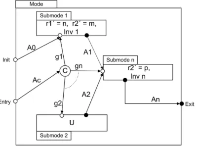
Main artifacts of REMES are modes. A mode is bound to a component and describes its behavior. Modes could be composite or atomic. A composite mode can contain multiple atomic modes. Atomic modes are also called submodes. A mode has data interface represented by global typed variables. Modes also have control interface defined by an entry and exit point. Exit point can have outgoing connections (edges) to other modes and entry points could have incoming edges from other modes. Edges represent the execution flow. An edge carries additional information - it has a guard condition and action body. A composite mode has an initialization point as well. The initialization (init) point is used for mode initialization. An outgoing edge from the init point to a submode indicates that the submode will be executed when mode is initialized. Modes could have constants and resources declarations. Remes mode could contain conditional connectors, which
12
are used to fork the execution flow depending on certain condition. Figure 2-3 shows a REMES composite mode.
Figure 2-3 REMES Composite Mode 2.1.3 Timed Automata
A timed automata (TA) is a finite state automata, to which a set of clocks is assigned. Those clocks start at zero and evolve continuously at fixed rate, and could be tested or reset to zero. TA consists of finite set of locations, connected via transition edges. Locations have invariants – clock constraints, which enforce that the location is left before constraint is violated. Guards are boolean conditions, assigned to transitions. Transitions can be delay or discrete. Delay transitions are result of passage of time while staying at some location. Discrete transitions are result of following an enabled edge in a TA to its destination location with the clocks in the reset set, set to zero. Systems comprising multiple concurrent processes are modeled by networks of timed automata, which execute with interleaving semantics and synchronize on channels. A good example of timed automata is described in [3]. Figure 2-4 shows the example.
13
Figure 2-4 Lamp-User Timed Automata
The example shows a system of two timed automations – lamp and user, modeling a scenario where the user presses a switch once for dim light and twice for bright light. The lamp stays dim for 10 time units after that goes off. The lamp has three states – off, dim and bright. Communication is done via synchronization channel “press”. Sending is denoted with “!” and receiving with “?”. A clock “t” is introduced. It’s reset to zero when the user presses the switch once and the lamp goes into the dim state. If the user presses the switch once more within 5 time units the lamp goes into the bright state. An invariant is assigned to the dim state, which will force the lamp back to the off state after 10 time units.
2.1.4 Priced Timed Automata
Priced Timed Automata extend TA with prices/costs on locations and edges. The cost for a location is the price per time unit for staying in that location. The cost for an edge is the price for taking the transition. A global cost is the accumulated price during the run of the automation. Multi-priced automata are extension of PTA, in which more than one cost variable exists. Figure 2-5 shows an example of a PTA.
14
Figure 2-5 Lamp-User Timed Automata extended with cost
Same example could illustrate the concept of PTA [3]. In the example the energy consumption is the cost. Switching the lamp on have energy consumption of 50 units, thus the corresponding transition increases the cost variables with 50. Staying in dim and bright locations is associated with linear consumption of energy over time – 10 units for dim and 20 units for bright locations.
15
2.2 Technological Background
2.2.1 UPPAAL
UPPAAL [4] is an integrated tool environment for modeling, validation and verification of real-time systems modeled as networks of timed automata, extended with data types (bounded integers, arrays, etc.). The tool is developed in collaboration between the Department of Information Technology at Uppsala University, Sweden and the Department of Computer Science at Aalborg University in Denmark. UPPAAL provides a core (server) component, which performs the analysis and verification of the TA system. The frontend (client) is realized as a client in Swing and communicates with the UPPAAL Server via specific protocol. To facilitate the client communication, UPPAAL provides API to access the server and allows easy reuse of the Core component in other applications. There is a family of UPPAAL products (CORA, TIGA, TRON), which provides extended functionalities the base UPPAAL application. UPPAAL provides a command line interface as well (verifyta). It is a stand-alone verifier, appropriate for e.g. batch verifications, and it’s out of scope of our integration. The UPPAAL frontend (client) provides three main functions - modeling of a PTA system, analysis and verification of the modeled system.
UPPAAL modeling language extends timed automata with some additional features such as bounded integer variables, binary and broadcast synchronization channels, urgent and commited locations. Bounded integer variables are declared as int[min,max] name, where min and max are the lower and upper bound, respectively. The bounds are checked upon verification and violating a bound leads to an invalid state that is discarded (at run-time). Binary synchronisation channels are declared as chan c. An edge labeled with c! synchronises with another labelled c?. Broadcast channels are declared as broadcast chan c. In a broadcast synchronisation one sender c! can synchronize with an arbitrary number of receivers c?. If there are no receivers, the sender could still execute c!, broadcast sending is non-blocking. Urgent synchronization channels are declared by prefixing the channel declaration with the keyword urgent. Delays must not occur if a
16
synchronization transition on an urgent channel is enabled. Urgent locations are semantically equivalent to adding an extra clock x, that is reset on all incoming edges, and having an invariant x<=0 on the location. Hence, time is not allowed to pass when the system is in an urgent location. Committed locations are even more restrictive on the execution than urgent locations. A state is committed if any of the locations in the state is committed. A committed state cannot delay and the next transition must involve an outgoing edge of at least one of the committed locations.
The UPPAAL model checker verifies a TA model against a requirements specification. The requirements specification is expressed using a query language. The query is used to verify whether certain property of the model is satisfied. Properties could be divided in three categories: reachability, safety and liveness. Reachability properties ask whether there exist a path starting at the initial state, such that certain condition is eventually satisfied along that path. Safety properties are on the form: “something bad will never happen”. For instance, in a model of a nuclear power plant, a safety property might be that the operating temperature is always under a certain threshold. Liveness properties are of the form: something will eventually happen, for example in a model of a communication protocol, any message that has been sent should eventually be received.
2.2.2 Eclipse
Eclipse [5] is an open source development framework for rich client desktop application. It’s implemented in Java and has a specific component model. Each piece of functionality is bundled in a plug-in. Figure 2-6 shows the Eclipse platform architecture.
17
Figure 2-6 Eclipse Platform Overview
Eclipse platform has a set of plugins, which provide the core functionality. New plugins contribute new functionality via so called extension points. For example menus, toolbars, action, etc. are contributed via extension points. To extend the Eclipse platform a plugin has to describe its functionality in a XML plugin descriptor. It specifies the extension point by id and other information required by the extension point. Most important is the fully qualified name of the java class, which implements the actual functionality. The plugin.xml file is the plugin “passport” to Eclipse.
The Eclipse user interface is organized in Perspectives. A perspective is a set of views, actions, menus and toolbars which serve to accomplish specific task or set of tasks. For example there is a Java, C and Subversion perspective. Views and actions are reused between perspectives, and for certain perspective only the relevant are shown. A view in Eclipse is a graphical component, which can show some content usually in read-only mode. It has to implement org.eclipse.views.IViewPart.
Eclipse uses Standard Widget Toolkit (SWT) library for rendering user interface controls. The JFace library further extends SWT to provide
Model-View-18
Controller (MVC) pattern via so called JFace viewer. A viewer has underlying SWT component, which is rendered on the screen - table for TableViewer, tree for TreeViewer, etc. This component acts as a view in the MVC pattern. A viewer has to be supplied with:
• content provider - it’s the controller in the MVC pattern, which knows about the model and is responsible for updating the viewer whenever the model changes.
• label provider - provides text and images for visual representation of model objects.
• input - the model which is loaded in the viewer. 2.2.3 Eclipse Launching Framework
Launching framework in Eclipse provides the tool developer with a way to launch a program or process and get feedback about its execution. The main part of the launching framework is the definition of new launch configurations. A launch configuration has type, mode and parameters. For example the Java launch configuration have run or debug mode and has many parameters, most important - the class to be run, the class path, the arguments to the Java Virtual Machine, etc. In a similar way any tool could contribute its own launch configuration and specify what to be launched, with what parameters and implement the actual launch. The eclipse framework gathers all launch configurations contributed via plugin descriptors and makes them visible in a unified way via the Run/Debug configurations dialog. Each launch configuration is persisted by Eclipse, this means that user could have multiple Java launch configurations and access them at any time, without the need to define again the VM arguments, class path, etc. The main points to contribute a launch configuration are the following:
• define a new launch configuration type in the plugin descriptor via the “org.eclipse.debug.core.launchConfigurationTypes” extension point. The extension point requires to provide an implementation of org.eclipse.debug.core.model.ILaunchConfigurationDelegate interface. The delegate is responsible to perform the launch given the parameters specified by the user.
19
• define a launch configuration tab group in the plugin descriptor via “org.eclipse.debug.ui.launchConfigurationTabGroups” extension point. The tab group is responsible to create the UI which will allow the user to configure the launch. The UI is organized in separate tabs. The tab group has to specify for which launch configuration type it is applicable. Separating the launch configuration type and the tab groups in different extension points provides loose coupling and allows different the tab groups to be reused by the launch configurations. 2.2.4 Eclipse Modeling Framework
The Eclipse Modeling Framework (EMF) [6] provides a set of classes and interfaces, which serve to enable Model-Driven Development. It has extensive tooling support, which allows models to be visually constructed and then Java source code to be derived easily. EMF provides developer with API for:
o Reflection - generic access of the model elements
o Persistence – using XML Metadata Interchange (XMI) standard format.
o Transactions – allows implementation of undo/redo via command stack.
o Change notifications – comes for free in the generated EMF models. 2.2.5 Graphical Modeling Framework
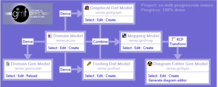
The Graphical Modeling Framework (GFM) [6] provides powerful runtime and designtime for creation of Graphical Editors for the Eclipse platform. Developing a graphical editor based on GMF follows certain workflow in which different artifacts are created or derived by combining other artifacts. The java code of the editor is then generated out of the GMF models. The developer could still make changes to the generated code. In order this custom code to be preserved in consequent generation, we should add @generated not annotation to the changed method or class. Figure 2-7 shows the GMF dashboard, which is a view in Eclipse and is a good illustration of the GMF development workflow.
20
Figure 2-7 GMF Dashboard
The starting point of the workflow is the domain model. Then the Graphical definition model and the tooling definition models are automatically derived from the domain model and usually require some customizations. The graphical definition model contains all figures, shapes, labels, etc. – graphical elements which will represent the domain model to the user. Their properties such as color, font and dimensions are specified as well. The tooling definition model is much simpler, it defines the palette – the container with tools next to the diagram sheet, from which the user could create domain model entities by drag and drop. Those two models together with the domain model are used to define the mapping model. The mapping model actually binds the both models to the domain model. This binding will define how domain model elements maps to their graphical representation, as well as what palette tool is used for creation. Such decoupling of models allows for example one complex graphical definition model to be reused across different domain models to create unified representation. Finally the mapping model is automatically transformed by GMF to a generation model. This model is the analog of Platform Specific Model (PSM) in MDA terms. In it we could specify properties, which are relevant to the target platform such as java package names, eclipse plugin names, etc. The final step is the generation of the editor as Eclipse plugin.
21 2.2.6 Object Constraint Language
The Object Constraint Language (OCL) [7] is a formal language, which is used to describe expressions on UML models. It has been developed as a business modeling language within the IBM Insurance division. Its main purpose is to bridge the gap between the complexity of traditional formal languages and the average business or system modeler. A formal language is used in software system modeling in order to specify invariant conditions that must hold for the system being modeled or queries over objects described in a model. A UML diagram, such as a class diagram, is typically not refined enough to provide all the relevant aspects of a specification.
OCL is a pure specification language - it is not possible to write program logic or flow control in OCL. When an OCL expression is evaluated, it simply returns a value and cannot change anything in the model.
In this thesis OCL is used to define certain constraints in the developed models. Also the transformation language introduced in the next section is partly based on OCL.
2.2.7 Atlas Transformation Language
In model-driven engineering a model is defined according to the semantics of a metamodel. It is said that the model conforms its metamodel. A model transformation aims to provide a mean to specify the way to produce a set of target models from a set of source models. For this purpose the transformation should define how the source elements are matched and navigated in order to create and initialize the target elements. Formally a model transformation has to define a way for generating a model B conforming to a metamodel mB, from a model A conforming to a metamodel mA.
Atlas transformation language (ATL) [8] is a model transformation language and a toolkit. An ATL transformation program (module) is composed of the following elements:
• Header section - defines the name of the transformation module and the variables corresponding to the source and target models
22
• Optional import section - enables to import existing ATL libraries; • Set of helpers - can be viewed as an ATL equivalent to Java methods; • Set of rules – defines the way target models are generated from
source ones.
An ATL helper may be called from different points of a transformation. It has name, context type, a set of parameters, return type and an ATL expression which is the helper body. For example a helper, which returns the value of an integer multiplied by n, would look like the following way:
helper context Integer def : multiplyBy(n : Integer) : Integer = self * n;
ATL provides two kind of rules - matched and called rules. Matched rules define for which kinds of source elements target elements should be generated and the way the generated target elements have to be initialized. For example we’ll look how a rule for transforming element Author conforming to metamodel MMAuthor to element Person conforming to metamodel MMPerson would look like:
rule Author { from a : MMAuthor!Author to p : MMPerson!Person ( name <- a.name, surname <- a.surname ) }
The source and target matching patterns are defined in the “from” and “to” sections respectively. Called rules could be seen as particular type of helpers, which generate target model elements. They are not directly invoked by the transformation, but we explicitly call them from another rule.
The ATL data type scheme is very close to the one defined by OCL. It has a set of primitive types, a hierarchy of collection types and a map type. Operations over variables are subset of operations defined by OCL and follow the classical dot notation:
self.operation_name(parameters)
23 2.2.8 Query-View-Transformation
Query-View-Transformation (QVT) [9] is a standard for model transformation defined by the Object Management Group. QVT is designed for transformations that have to build target models of a complex structure. It is convenient to be used in cases when there is no direct correspondence between individual elements of the source and target models. Such cases might be difficult to describe in declarative transformation languages such as ATL.
Eclipse provides an open source implementation of the QVT standard. A QVT transformation has a signature: transformation A2B (in A : mA, out B: mB). The signature defines the source and target models, and metamodels they conform to. Each transformation has one operation named “main”, which is the entry point and is called automatically after transformation instantiation. Mapping operations in QVT are responsible to transform source into target model elements. They are the alternative of called rules in ATL, and have following signature:
mapping mA::A::toB() : mB::B;
The given mapping defines transformation for element A of metamodel mA to element B of metamodel mB. The operation is invoked by using the dot notation on an instance of A, for example a.map toB();The mapping body defines the transformation itself.
QVT also defines queries and helper operations. More details here [ref]. 2.2.9 REMES GUI
The REMES GUI [10] is a graphical modeling tool for REMES. It allows user to create REMES model diagrams and insert, connect and edit modes, submodes and conditional connectors. It is developed as Eclipse plugin for the purpose to seamlessly integrate with the Progress IDE. REMES GUI uses EMF and GMF as tool development standards in Eclipse. The GUI is a result of previous work in the field.
Here is a brief description of the realization of the REMES GUI. It defines a metamodel for REMES instances in the Ecore metamodeling language. Java code for this metamodel is automatically generated by EMF. The REMES java metamodel
24
provides API for manipulating and persisting model instances in XMI format – a standard format for exchanging metadata. GMF is used for the development of the diagram editor. The REMES metamodel was supplied with several GMF models. Those include the graphical definition model, tooling definition model and the mapping model. They define how the model will be represented visually and how the editor will behave. GMF then generates java code for the editor as Eclipse plugin. Custom modifications were made to the generated code in certain places, where GMF was providing too generic functionality.
2.2.10 UPPAAL Modeling tools
The UPPAAL modeling tools [11] are set of plugins, which bring the following functionality and features in the Progress IDE:
• EMF-based UPPAAL metamodel. It is used to manipulate UPPAAL models and produces models ready to be loaded in the UPPAAL simulation/verification engine.
• EMF-based lightweight version of the UPPAAL metamodel (ULITE). It is a subset of the UPPAAL metamodel targeted for use within the Progress IDE. Its main purpose is to facilitate the transition from ProCom to PTA by simplifying the UPPAAL metamodel significantly. A diagram of the metamodel is available in the Appendix.
• GMF-based graphical editor for ULITE. It allows the user to create and edit PTA models in a diagram.
• ATL model to model transformations for converting a REMES model to an ULITE model and ULITE model to UPPAAL model.
• Actions and wizards, used to invoke the ATL transformations. The plugins contributed to the Progress IDE are:
• hr.fer.rasip.remes.* • hr.fer.rasip.uppaal.* • hr.fer.rasip.uppaallite.*
25
Current thesis relies heavily on the UPPAAL modeling tools and it contributes certain extensions to them in order to include the ProCom semantics in the REMES to ULITE transformation.
26 2.2.11 Attribute Framework
Attribute Framework [13] is specific to the Progress IDE and provides unified extensibility for ProCom models. It allows the user to assign various types of attributes to ProCom models during the development of a component of a system. Those attributes represents extra-functional properties, which are not described by the ProCom metamodel. The framework maintains a list of attribute types in a registry. The specification of an attribute includes the list of the entities to which the attribute could be attached and the valid format of the attribute values.
The Attribute framework is a plugin in Progress IDE, and provides set of Eclipse extension points, Java interfaces and base classes in order new attribute types to be contributed.
27
3 Problem Analysis
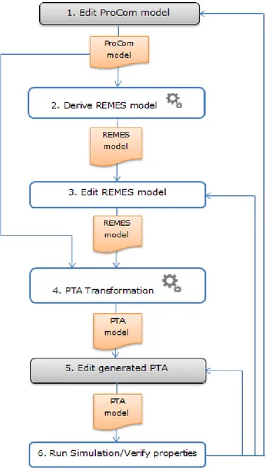
Figure 3-1 will help to gain insight into the problem and its scope. It illustrates the workflow, which will be performed by the user. The workflow starts with the ProCom model editors and finishes when the simulation is run and results are available. Depending on the results, the workflow might be repeated.
28
In the terms of the Unified Modeling Language (UML) there is one actor – the embedded system designer. All depicted activities happen inside the Progress IDE. Some of them are annotated with gear icon. Those are automatic activities, which are invoked by the user. Some of the activities have gray background – they are out of the thesis scope. Activities provide output to each other.
The tools for performing the first activity are already in place. It’s handled by ProCom model editors. In the next sections higher detail requirements are extracted.
3.1 Integration between ProCom and REMES
The second activity ‘Derive REMES model’ should be performed automatically and should use the ProCom model to produce REMES template model. The template model should contain one top-level composite mode corresponding to one ProSys/ProSave component. Component interface should be mapped to REMES variables. The mapping should be done in different way for ProSave and ProSys components. For ProSave components, each trigger port should be mapped to a REMES boolean variable, and each data port should be mapped to a REMES data variable of same type as the port type [14]. ProSys components communicate via asynchronous messages sent via typed message channels. Each message port should be mapped to a pair of REMES variables – one boolean variable representing data availability and other variable with same type as the data port. Figure 3-2 shows an example mapping. The mapping is covered in more details in [14].
ProSys port REMES variables A1 bool A1 and float A1_value
A2 bool A2
A3 bool A3 and int A3_value
29
In addition the derived REMES model should be assigned as attribute to the corresponding ProCom component. This imposes the need for registering new attribute type ‘Behavior model’ in the attributes repository.
3.2 REMES GUI Extension
The third activity ‘Edit REMES model’ involves using the REMES GUI. The first REMES GUI version [10] provides only rough support for declaration of variables, resources and constants (referable entities). They were declared as free text. In order to implement the PTA transformation, referable entities have to be included in the REMES model with more metadata, such as type, expression and additional properties. This would make possible for the transformation to reflect them in the generated PTA. From the visual aspect they should reside in own compartments in the diagram elements and user should be able to create and manipulate them in the editor. There should be several types of resources (memory or port – discrete resources, cpu, bandwidth or power – continuous resources). Variable types should be boolean, integer, natural or clock. The clock is a special type, which is used to define clock variables evolving at fixed rate.
ProCom components can provide multiple services, and each service can have a single input port group (trigger port + N data ports) and multiple output port groups. Each service behavior is modeled by a composite mode in REMES. In the current REMES design mode execution enters through entry point, reads input variables from ports, then executes submodes and exits through exit point (writing output variables to ports). ProCom however allows different output groups to be activated at different time [15]. This brings the need to introduce an additional control point in the REMES metamodel – a write point. A connection to the write point means that output variables are written to ports before the mode is reentered. With write points REMES execution flow goes like this: enter the mode, read input ports, execute, write output ports, execute, write output ports …, exit. This aligns REMES execution semantics with ProCom by ensuring that for each activated service, every output port group is activated exactly once.
30
The write point is kind of "local" exit point, where the current state is written to output ports in contrast to the "global" exit point, where it's known that all outputs have been set, the mode execution can finish and service can go idle.
The initial REMES metamodel version [10] relied on classification of connection edges, depending on the connection source and target. For example an edge could be ‘Entry Conditional Top Edge’, meaning that it connects an entry point of a composite mode with an entry point of a conditional connector. Such approach was not convenient for the PTA transformation and for the user. In order to create a connection in the diagram, user would have to select the appropriate connection tool depending on what entities will be connected. This posed the requirement to refactor the metamodel by introducing control point entities, and making edges connect from one point to another.
3.3 PTA Transformation
The fourth activity ‘Transform to PTA’ should take as input the ProCom model and its REMES behavior model and generate a PTA model. Our task is to identify those pieces of ProCom metadata, which should be taken in account when transforming the REMES model to PTA, and to implement the corresponding rules as part of the existing [11] or in a new ATL transformation. A prerequisite for the transformation is the development of the PTA metamodel [11]. We have identified that the transformation should implement the following rules [12]:
• A REMES diagram should transformed into a network of PTA • A composite mode should be transformed into a single PTA.
• REMES control points, as well as submodes should be transformed into PTA locations.
• REMES edges should be transformed into PTA edges.
• Variables for passing control in REMES should be transformed to synchronization channels in PTA.
• Data variables should be transformed to PTA variables. Their type should be mapped to the corresponding type in UPPAAL.
31
• REMES Resources should be reflected in the cost function calculation in the generated PTA diagram.
• An additional start location is added to each PTA as well as dedicated PTA template for initialization.
User is able to edit the generated PTA model in the fifth step. The corresponding editors are out of scope for the current thesis. They have been developed as result of [11]. By editing the generated PTA model, user is able to better reflect the semantic of the system design in the PTA model.
3.4 UPPAAL Integration
To accomplish the last step in the workflow - ‘Run Simulation’, user should be able to launch the PTA model in the UPPAAL tool. One of the tasks in the thesis scope is to provide a wrapper of the UPPAAL tool, so that it is available in the Progress IDE. This would provide unified user experience. Following requirements were identified:
• User should be able to start UPPAAL simulation for a PTA model and observe the resulting visual trace.
• User should be able to view enabled transitions for a selected state in the trace.
• User should be able to control the simulation by switching manually to different transition, thus navigating the execution path.
• User should be able to view automatic execution of the simulation, where trace is constructed by choosing random transition from the set of enabled transitions for the current state.
• User should be able to launch UPPAAL verifier to check a PTA model against certain set of properties. Verification results should be presented to the user.
32
4 Solution Design
The chapter describes the prototype design and realization. It is divided in four parts, which cover the four main sub-goals – to integrate REMES with ProCom, to extend the REMES GUI, to implement the PTA transformation and to integrate the UPPAAL CORA tool in the Progress IDE.
4.1 Integration between ProCom and REMES
The integration between ProCom and REMES is done via the Attribute Framework in Progress IDE and the QVT transformation language. The integration is realized as Eclipse plugin - se.mdh.progresside.remes.attributes. The main goals are to provide mapping between a ProCom component and a REMES model defining the component’s behavior and to provide generation of a template REMES model out of a ProCom component.
The plugin defines a new attribute category named “Behavior” by contributing to the se.mdh.progresside.attributes.framework.categories extension points. Two attributes are then defined in this category by using the se.mdh.progresside.attributes.framework.registration extension point. The first attribute allows REMES models to be attached to ProSys subsystems, and the second – to ProSave components. Attribute value is the local path of the REMES model file within the ProCom project. Figure 3-3 shows a Temperature Control System project with several ProSave components created. There is one REMES model per component located in the \models\REMES\component.remes file, relative to the respective component.
33
Figure 3-3 Sample ProCom project structure
Another responsibility of the integration plugin is to automatically produce a template REMES model per ProSave components and ProSys subsystems. This is achieved by a model to model transformation implemented in Eclipse QVT. There is no specific motivation behind using QVT and not ATL for this transformation. QVT syntax is closer to the object oriented / procedural languages, while ATL has mainly declarative syntax. This makes QVT easy and convenient to use for small and
relatively simple transformations such as the generation of REMES template models out of ProCom components.
The transformation, which maps ProSave component to REMES model is realized in mapsProSaveToREMES.qvto file. It defines the following mappings:
mapping ProComMM::proSave::InputTriggerPort::toVariable() : REMESMM::Variable mapping ProComMM::proSave::OutputTriggerPort::toVariable() :
REMESMM::Variable
mapping ProComMM::proSave::InputDataPort::toVariable() : REMESMM::Variable mapping ProComMM::proSave::OutputDataPort::toVariable() : REMESMM::Variable mapping ProComMM::proSave::Component::toCompositeMode() :
REMESMM::CompositeMode
First four mappings transform ProSave component ports to REMES variables. Variables are initialized depending on the port kind (input or output, data or trigger). For example output trigger port is mapped to Boolean, writable variable,
34
while an input data port is mapped to a read-only variable. The type of the variable is obtained by mapping the data port type to the corresponding REMES primitive type. The last mapping creates blank composite mode, pre-initialized with the default set of control points. The transformation has a main subroutine, which iterates all the ports and creates the corresponding REMES variables.
The generated REMES model acts as a stub, which is later edited by the user. The user could modify the components interface by adding/removing/editing ports for example. When consequently triggered, the transformation will try to detect the existing REMES variables and modes and preserve custom user changes. This is done by queries and checks in the transformation.
The transformation, which is responsible for mapping ProSys subsystem to REMES model is realized in mapsProSysToREMES.qvto file. In a similar way it iterates through the subsystem ports and creates or updates the corresponding REMES variables. The difference is that as pointed by the requirements in the previous chapter, message ports are iterated and two variables are generated for each port.
Possible improvement of the transformations could involve refactoring by moving common subroutines in a separate library transformation and then reused.
4.2 REMES GUI extensions
The REMES GUI is realized in the following four plugins:
• se.mdh.progresside.remes – contains the REMES metamodel (EMF model file and the generated Java classes for model manipulation) and the GMF definition of the REMES diagram editor. The GMF model spans across three separate model files – remes.gmfgraph, remes.gmftool and remes.gmfmap.
• se.mdh.progresside.remes.edit, se.mdh.progresside.remes.editor – supporting plugins generated by EMF, which contains helpers and utilities for REMES model manipulation.
35
• se.mdh.progresside.remes.diagram – contains generated Java classes for the REMES diagram editor.
Following sections describe the different aspects in which the REMES GUI was extended.
4.2.1 Definition of constants, variables and resources
Figure 4-1 depicts the new artifacts, which were added to the REMES metamodel. It is an excerpt of the whole metamodel to illustrate only variables, constants and resources (referable entities).
Figure 4-1 Referable entities in REMES metamodel
The Referable interface contains single property ‘name’, and is extended by Variable, Resource and Constant. Variable have primitive type. Property ‘vectorSize’ is greater than zero if the variable is an array. The ‘readable’ and ‘writable’ flags determine whether the variable represent input or output port in ProCom semantics. Resources have ‘type’ and ‘expression’ properties. If the resource is continuous, then the expression property defines the rate at which the resource is being consumed. The rate is defined by the first derivative of the resource.
REMES diagram editor had to be extended as well in order to allow constants, variables and resources to be manipulated. Both graphical definition and mapping
36
model (defined in remes.gmfgraph and remes.gmfmap files respectively) were modified. The graphical definition already contained shapes, which would represent REMES modes in diagram. For both composite modes and submodes we created compartments for variables, constants and resources. In the mapping model we had to add compartment mappings. They define that composite mode variables should be displayed in the variables compartment, resources in resources compartment, etc.
Figure 4-2 shows how a metamodel entity (composite mode) is mapped to its graphical representation via the mapping model. The GMF mapping model allows expressing diagram editor behavior in a declarative way.
Figure 4-2 Compartment mappings in the GMF mapping model
Figure 4-3 shows how a compartment mapping is defined in the GMF mapping editor via the properties view. In the children property we have to provide a reference to the element of the domain model (REMES metamodel) and in the
GMF Mapping Model Graphical definition model
Composite mode rectangle Variables compartment … Variable label Variable label Submodes compartment Submode rectangle REMES Metamodel Composite mode Variables (0..n) … Submodes (0..n) Submode rectangle Compartment mapping Compartment mapping Node mapping
37
visual representation, we have to provide a reference to a graphical shape which will show the compartment.
Figure 4-3 Definition of compartments in the properties view
The next figure shows how the mapping model was customized to achieve in-place editing for constants.
Figure 4-4 Definition of in-place editing for constants
GMF allows two sets of features to be specified – features to be displayed and features for edit. A feature in this case is any property of the constant object. We have specified that constant name, type and value will be displayed and the name and value will be edited. We specify certain formats for display and edit. The selected method “MESSAGE_FORMAT” allows us to use a standard format pattern. According to the edit pattern the user input will be parsed. The view pattern specifies how the constant object will be displayed in the label. For example if we have created constant ‘limit’ of type ‘integer’ with value 20, it will be displayed according to the view pattern as “limit=20(integer)”. If user enters “limitRenamed=30” then the input will be parsed according to the pattern
38
{0}={1}, and the constant name will be set to limitRenamed and the value to 30. Similar modifications were done for variables and resources as well.
To specify custom icons for resources depending on their type (CPU, bandwidth, power, port or memory) we had to modify the generated getLabelIcon method for the resources edit parts and annotate it with @generated NOT. Edit parts are java classes generated by GMF, which handle visualization and behavior of certain model elements in diagram (in this case resources).
4.2.2 Introduction of Control Points
Figure 4-5 shows a metamodel excerpt with the introduced entities in the metamodel.
39
Four types of points were introduced in the metamodel: entry and exit points, init and write points. An edge connects an exit point to an entry point and has action guard and action body properties. Modes (composite and atomic) and conditional connector contain an entry and an exit point, which is used respectively to enter and exit the mode/connector. A composite mode in addition has an init point, through which the initialization is done, and a write point, which serves as a local exit point as discussed earlier. The init point is connected to an entry point via init edge and a write edge connects an exit point to the write point.
Figure 4-6 helps to get better understanding how the metamodel maps to a model instance.
Figure 4-6 Control points legend
The composite entry and exit points deserve closer look. A composite mode is entered via its regular entry point. In model semantics it’s not possible to connect this entry point to another entry point, for example of a submode. An edge only connects exit point to entry point. This imposed the need to introduce “intermediate” points – the CompositeEntryPoint and CompositeExitPoint. Note that composite entry point extends ExitPoint in order to allow them to be user as source of an edge. Similar applies to the CompositeExitPoint – it extends EntryPoint, so that it could be the target of an edge.
Changes in the generated EMF editor code.
Control points are metamodel entities, which require special behavior in regards to tooling. REMES model editing was enhanced in a way that when new composite mode, submode or conditional connector is created, it should have
40
predefined entry and exit points. Composite modes should have as well init, write, composite entry and composite exit points pre-created. To achieve this, a custom code was contributed in parallel to the generated by EMF editor code. The responsible class is se.mdh.progresside.remes.util.RemesDefaultElementFactory. It is invoked when a new model entity is created in order to pre-create and attach the corresponding control point. This factory is located in the edit plugin, generated by EMF (se.mdh.progresside.remes.edit) and is reused in the diagram editor.
Changes in the GMF model.
As we have introduced new entities in the REMES metamodel we had to update the graphical definition model by adding a node for each type of control point. The mapping model had to be updated as well, so that points were mapped to the corresponding nodes from the graphical definition model. At this stage the control points would appear inside the modes, as hierarchically they are contained within modes. We want them to be attached to the mode borders instead. For this we had to specify the “Affixed Parent Side” property of nodes in the graphical definition model. This property has four possible values – EAST, WEST, SOUTH and NORTH and tells GMF to attach the node to the border of its parent. For example the node which represents the init point has specified “WEST” as affixed parent side, so that this point will be displayed in the left border of its parent composite mode.
By default the GMF generated diagram editor would allow used to delete the control points from diagram. This would lead to invalid models, thus we had to disable this behavior. To achieve this we had to add the following code to the createDefaultEditPolicies method of control points edit parts:
installEditPolicy(EditPolicy.COMPONENT_ROLE, new ComponentEditPolicy() { protected Command getDeleteCommand(GroupRequest request) {
return UnexecutableCommand.INSTANCE; }
});
In addition the semantic edit policy of each control point has been modified as well. The getDestroyElementCommand was modified and annotated with @generated NOT statement:
41
/**
* @generated NOT */
protected Command getDestroyElementCommand(DestroyElementRequest req) { return UnexecutableCommand.INSTANCE;
}
A semantic edit policy is a class in GMF responsible to handle creation and update of semantic model elements.
With the introduction of control points the classification of edges was replaced by three types of edges – init edge, connecting init point with some internal mode, write edge and a regular edge. Due to the fact that edges specify in very generic way its source and target in metamodel (they connect control point to control point), we had to define additional constraints. This would prevent the user to create invalid edges for example from the exit point of a submode to the entry point of a submode located in another composite mode. Those constraints were defined in the GMF mapping model by adding OCL constraints for link mappings. Link mappings define what connection could exist in the diagram and between what kinds of nodes. The mapping model contains three link mappings for each type of edge. As an example let’s take a look at the link mapping describing the init edges. The link mapping is associated with the InitEdge metamodel element and connects init point to an entry point. We should ensure that the init point could be connected only to an entry point of a submode or conditional connector which is located inside the composite mode. This is illustrated on figure 4-7. The invalid edge is outlined:
42 The corresponding OCL constraint is:
(self.container.oclIsTypeOf(SubMode) and
self.container.oclAsType(SubMode).parent=oppositeEnd.container) or
(self.container.oclIsTypeOf(ConditionalConnector) and
self.container.oclAsType(ConditionalConnector).parent=oppositeEnd.container)
Basically the constraint handles two cases – when the target is submode and when the target is conditional connector. In both cases, the target’s parent should be the same as the container of the init point (the composite mode).
OCL constrains for the other link mappings are defined in a similar manner. Some constraints are heavy and hard to understand and develop. Testing and development of OCL constraint was greatly facilitated by the Interactive OCL console for Eclipse. It allows executing OCL queries against live EMF model instances.
43
4.3 PTA transformation
One of the thesis goals is to extend the existing ATL transformation [11], so that it reflects the integration of ProCom with REMES. There are several things that should be reflected in the generated PTA diagram. They are covered in the following sections.
4.3.1 Reflecting ProSave components communication in PTA
Here we present the following example, to illustrate a specific aspect of transformation from REMES and ProCom to PTA.
Example
We have composite ProSave component consisting of two primitive components C1 and C2, shown on figure 4-8.
Figure 4-8 ProSave component communication example
Both C1 and C2 have data ports named ‘dataIn’ and ‘dataOut’ respectively. When component C1 sends a signal to C2 over the output trigger port, the value of C1 output data port is read and written to C2 input data port. This communication is reflected in the resulting PTA model via synchronization channels and update of global variables.
When the ProSave components are transformed to PTA, two PTA templates are created for each of them. Figures 4-9 and 4-10 shows the generated PTA templates.
44
Figure 4-9 PTA template for C1 component
Figure 4-10 PTA template for C2 component
We can see that when component C1 is exited a synchronization message is sent over the Sync_C1Exit channel. The C2 PTA waits for this message and when received it reenters the Entry location and executes update “I_dataIn = C1_dataOut”. This will write the value of the variable representing the C1 output data port to the variable representing the C2 input data port. Those variables, as well as the synchronization channels are defined in the resulting PTA diagram on a global level.
The channel “t” is an initialization synchronization channel. The synchronization “t!” is sent in specially generated initialization template, which has a sole purpose to trigger the initialization of all templates in the PTA system. Each of them has “t?” in its initialization transition.
45 Implementation
In this section we cover the main implementation details regarding the described transformation. To reflect the connection from C1 to C2, we introduced some additional rules in the transformation. When constructing the transition from Idle to Entry (reentering a REMES mode), we check whether the corresponding ProSave component has input trigger port. If this is the case, then we insert synchronization “SyncID?” in order to enforce the transition when this input trigger has been activated. To identify the synchronization channel we use the ID of the ProSave trigger in the EMF model. In addition we check whether we have to associate an update to the transition, so that the variables corresponding to the data ports are updated. The check is done by querying the ProSave model to find whether there is a ProSave component which output data port connects to the current ProSave component (the one being processed by the transformation currently). We make similar check to find whether we have to insert synchronization trigger “SyncID!” when exiting a mode. In this case the synchronization must signal to other possibly connected ProSave components, that the current component has finished execution. The check tries to find an output trigger port associated with the current ProSave component.
Next we list the helpers introduced in the ATL transformation. First there are executed in the context of the context of a specific REMES mode, while the last two are global, they are defined in the scope of the current models being transformed.
helper context REMES!Mode def: inputSync() : String
helper context REMES!Mode def: assignmentOnInputSync() : String helper context REMES!Mode def: outputSync() : String
helper def: triggersToSyncChannels() : String
helper def: outputDataPortsToGlobalVars() : String
4.3.2 Reflecting ProSys components communication in PTA
In ProSys, components communicate via message channels. This reflects the transformation in a specific way and we will illustrate it with the following example.
Example
We have four primitive ProSys components used in one composite ProSys subsystem shown on figure 4-11.
46
Figure 4-11 ProSys component communication example
Components C1 and C2 send messages to C3 and C4 via the message channel MC. The specific thing here is that the resulting PTA diagram contains an additional template for the message channel. The next figure shows how the generated PTA template looks like.
Figure 4-12 Generated PTA template for message channel
The template contains single location and two transitions. The first transition is executed whenever “Syn_C1Exit” synchronization is received. It corresponds to the connection from component C1 to the message channel. In this case the input ports of the C3 and C4 components need to be updated. This is done by the update statement assigned to the transition. Since each ProSys port maps to a pair of variables, and there are two outgoing connections from the message port, four variables in total are updated. Similarly the second transition corresponds to the connection from C2 to the message channel and it waits for the “Syn_C2Exit” synchronization to be triggered, which should happen when the C2 component is exited. If we examine the generated PTA template for the C2 component on figure
47
4-13, we will see that the transformation has inserted a “Syn_C2Exit!” trigger when the exit location has been left. Note that there are no start and init locations in the PTA. This is because the assigned REMES model for C2 does not contain initialization edge.
Figure 4-13 PTA template for C2 ProSys component
The example illustrates another aspect of the transformation. Certain modes in REMES are non-lazy modes. A non-lazy mode does not specify invariant and does not have a constraint on how long the execution could delay in that mode. To avoid situation, where the execution could stay forever in such mode a special synchronization channel was introduced (Syn_nonLazy in the figure). Such channel is inserted into the generated PTA is a non-lazy mode is detected in the REMES model, and an additional PTA template called NonLazyModeSynchronizer is generated. It has only one urgent location which exits immediately and triggers synchronization message via the Syn_nonLazy channel. The template is shown in figure 4-14.
48 Implementation
To implement the covered functionality as ATL transformation, some additional rules and helpers were introduced. The rule messageChannel2Template
transforms a ProSys message channel to template in UPPAAL Lite model. The rule uses the syncTransitions helper, which creates one PTA transition per each
incoming connection to the message channel. A synchronization trigger “Syn_ID!” is assigned to each transition, where the ID is the EMF model ID of the output message port, which connects to the message channel. In the given example a transition is created for C1 and C2. In addition the helper syncTransitionAssign
calculates the update statement, which should be assigned to the transition to update the variable values. The helper relies that variable names are derived according to certain convention out of the ProSys message ports. Same convention is used by the QVT transformation, which translates ProSys component to REMES behavior model. Variable name is concatenation of ProSys component name, underscore and the input message port name.
The rule nonLazyModeSynchronizerTemplate creates the template for
synchronizing non-lazy REMES modes. In addition, when an outgoing transition is being created for a non-lazy mode, a “Syn_nonLazy?” synchronization is assigned to the transition.
4.3.3 Translating Clocks into PTA
When modeling a ProSys subsystem, clocks could be inserted in the diagram. Clocks are special type of connector components, which does not have output data port, but only one trigger port. The trigger signal is generated on certain period, which might be specified by the user. Figure 4-15 shows such example.
Figure 4-15 Example of ProSys component with Clock
For each clock in the ProCom model, a dedicated PTA template is generated during the transformation, shown on figure 4-16.
49
Figure 4-16 PTA template for Clock
The clock template has single location with invariant x <= P. The template has declaration “clock x; const int P =0;”, which defines the x as clock variable in UPPAAL and the period as defined in the Clock component in ProCom. When the invariant does not hold anymore (the elapsed time is greater than P) the transition will be executed, which will reset the clock to zero and trigger synchronization over the “Syn_Clock” channel. This channel is defined globally on PTA system level and is used in component C1 as synchronization on re-entry. Figure 4-17 shows the generated PTA template.
Figure 4-17 PTA template for component connected with clock
From ATL perspective, an additional rule Clock2Template was introduced,
which translates ProSave clock to PTA template. The synchronization is handled by the existing transformation rules, since the Clock is treated as regular ProSave component with output trigger port.