V¨
aster˚
as, Sweden
Thesis for the Degree of Master of Science in Engineering - Robotics
30.0 credits
OBJECT RECOGNITION THROUGH
CONVOLUTIONAL LEARNING FOR
FPGA
Daniel Jonasson
djn12001@student.mdh.se
Examiner: Masoud Daneshtalab
M¨
alardalen University, V¨
aster˚
as, Sweden
Supervisor: Ning Xiong
M¨
alardalen University, V¨
aster˚
as, Sweden
Company supervisor: Lars Asplund,
Unibap, V¨
aster˚
as, Sweden
Abstract
In later years the interest for deep networks and convolutional networks in regards to object recog-nition has spiked. There are however not many that focuses on the hardware in these subjects. This thesis was done in collaboration with Unibap to explore the feasibility of implementing these on a FPGA to speed up object recognition. A custom database is created to investigate if a smaller database could be utilized with good results. This database alongside the MNIST database are tested in multiple configurations to find a suitable solution with good enough accuracy. This thesis fo-cuses on getting an accuracy which could be applicable in industries of today and is therefore not as driven by accuracy as many other works. Furthermore a FPGA implementation that is ver-satile and flexible enough to utilize regardless of network configuration is built and simulated. To achieve this research was done on existing AI and the focus landed on convolutional neural net-works. The different configurations are all presented in regards to time, resource utilization and accuracy. The FPGA implementation in this work is only simulated and this leaves the desire and need to syntethize it on an actual FPGA.
Acronyms
AI Artificial Intelligence. ANN Artificial Neural Network.
CNN Convolutional Neural Network. CPU Central Processing Unit.
DCNN Deep Convolutional Neural Network. DNN Deep Neural Network.
FPGA Field Programmable Gate Array.
GD Gradient Descent.
GPGPU General-Purpose computing on Graphics Processing Units. GPU Graphical Processing Unit.
IVS-70 Intelligen Vision System-70.
LUT Look-Up Table.
RCNN Reccurent Convolutional Neural Network.
RDCNN Recurrent Deep Convolutional Neural Network. RLU Rectified Linear Units.
Table of Contents
1 Introduction 5
1.1 Problem Formulation . . . 5
1.1.1 General research problem . . . 5
1.1.2 Problem formulation . . . 5 2 Background. 7 2.1 Motivation . . . 7 2.2 Training data . . . 7 2.3 FPGA . . . 7 2.4 Existing methods . . . 8
2.4.1 Artificial Neural Network . . . 8
2.4.2 Convolutional Neural Network . . . 9
2.4.3 Recurrent Convolutional Neural Network . . . 9
2.4.4 Deep learning . . . 9
2.4.5 Related work for optimization and FPGA implementations . . . 10
2.4.6 Reasoning . . . 12
3 Method 13 3.1 Layout . . . 13
3.1.1 Deep Convolutional Neural Network . . . 13
3.1.2 Reccurent Deep Convolutional Neural Network . . . 14
3.2 Training . . . 15
3.2.1 Backpropagation - Fully connected layers . . . 15
3.2.2 Backpropagation - Max pooling layers . . . 16
3.2.3 Backpropagation - Convolutional layers . . . 16
3.2.4 Training data . . . 17
3.3 Implementation . . . 17
3.4 Analysis . . . 17
4 Hardware 18 4.1 Cameras . . . 18
4.2 Field Programmable Gate Array . . . 18
4.3 System on Chip . . . 18 5 Implementation 19 5.1 Testing . . . 19 5.1.1 MNIST . . . 19 5.1.2 Custom database . . . 19 5.1.3 Test setup . . . 19
5.2 Field Programmable Gate Array (FPGA) implementation . . . 20
5.2.1 Resources . . . 22
5.2.2 Timing . . . 23
6 results 24 6.1 General research problem . . . 24
6.1.1 Question 1 . . . 24 6.1.2 Question 2 . . . 24 6.1.3 Question 3 . . . 24 7 Discussions 26 7.1 Question 1 . . . 26 7.2 Question 2 . . . 26 7.3 Question 3 . . . 26 8 Future Work 27
9 conclusion 28
10 Acknowledgments 29
1
Introduction
In later years the interest in robotics have been growing. Although industry was the first to discover the advantages of using robots, more and more areas are becoming aware of the benefits of implementing robotics. Everything from production to health care. Even our homes are starting to make use of robotics in the form of vacuum cleaners, lawn mowers and other applications. This has driven the research community to look into the major obstacles in the field. One of the biggest hindrances to increasing the versatility of robotics of today is the lack of awareness in robots. If a robot were given the ability to see its surroundings and take decisions accordingly then the versatility would increase exponentially. One example could be having the manipulators in an assembly line be able to detect and pickup individual screws from out of a box. One of the core features to achieve this is object recognition. Although multiple methods for object detection exists today there is room for a lot of improvements. One of these improvements are to speed up the detection without losing efficiency.
This thesis is focused on finding a suitable Artificial Intelligence (AI), more specifically an
Artificial Neural Network (ANN) that may utilize deep learning [1], that is fast and reliable for implementation on a FPGA. The goal is to implement an AI that fulfills the requirements for a FPGA, fully or partly, on a simulated FPGA so that the parts intended for it can be easily synthetized and transferred to aFPGA. This implicates that one of the focuses of this thesis will be to ensure that the part of theAIintended for theFPGAis executable on it.
Included in this thesis are research of existing algorithms and methods for object detection intended for deployment on a FPGAand methods for reducing the load on computational com-plexity and memory usage. The implementation will be tested by a custom image training set as well as a well-known database and a proper analysis is included. This thesis was conducted in collaboration with Unibap [2] and is intended to, in the future, be integrated with their existing platform Intelligen Vision System-70 (IVS-70). In contrary to existing solutions this thesis will focus on finding a solution which can be easily re-trained on a small custom database so that it is versatile enough to be deployed at many different companies with different applications without the need for massive retraining or alteration. The training will be performed outside theFPGA
program as only the forward pass will be implemented on it. This will save resources and the training is optimally performed on a large server park or a super-computer.
1.1
Problem Formulation
Before work began a hypothesis was stipulated and some questions were formulated to give the scope of the thesis.
1.1.1 General research problem
What methods are feasible when implementing object recognition on aFPGA and which of these methods are the most suitable?
Not all methods will be considered but rather a few that are chosen from the research performed and requests from Unibap.
1.1.2 Problem formulation
The following questions are formulated to solve the general research problem.
Q1 What limitations does the FPGAentail?
Since the goal of this thesis is to find a method that fully or partly is implementable on a
FPGAit is imperative that the methods chosen are analyzed and compared to the specifica-tions of the hardware it is intended for.
Q2 Considering the limitations mentioned in Q1. What type of ANN is suitable? Whit the limitations in mind. What type of AI would fit within the limitations both in regard to size, complexity, accuracy and method.
Q3 Is it possible to fit the entire network on the FPGA?
With the intended hardware in mind. Is it plausible to fit the entire network on theFPGAor only part of it? If only part of it fits then what parts of the network should be implemented in theFPGA
2
Background.
The background is divided into five sections. The first section describes the company Unibap that proposed this thesis and why it was proposed. The second section describes the training data briefly. The next section describes FPGA, why it is a suitable hardware, and presents the limitations that needs to be considered when designing aANNintended for theFPGA. The fourth section presents the research done on existing solutions both intended forFPGAsas well as general methods for object recognition by utilizingANNs. Most of these are focused on optimization. The final section handles the reasoning and choice of method to implement in this work.
2.1
Motivation
Unibap are taking the step towards intelligent visual perception solutions and are already a world class supplier of safety critical solutions in vision processing. They started out in the aerospace marked and are now moving into the industrial machine vision market. One of the ideas they are working with is implementation of solutions that are inspired by artificial visual cortexes. Unibap believes that the future of automation lies with a robust and reliable vision system. As quoted on their website:
”Artificial intelligence and machine vision are key enablers of the future automation industry. The world market is rapidly growing according to almost all reports — intelligent machine vision for automation is the holy grail.”
This thesis were conceptualized because of this drive and the applications of such a solution is massive.
2.2
Training data
To train anANNa training data set, consisting of training and validation examples, is required. The training data examples are used to train the network while the validation examples are used to validate the training of the network. It is important to note that the sets needs to contain both positives (The object sought after) as well as negatives (other objects) to prevent false positives. If a network is supposed to recognize nails and it does not have the negatives in its training data set the network might classify similar objects, such as screws, as nails. It is also important that there is a sufficient amount of training data. A deep network especially is prone to suffer from overfitting if the training data is too small.
2.3
FPGA
There exists a lot of solutions to object recognition utilizingANNs. The problem however is that these networks demands a lot of computing power. This has spawned the need for a reduction in hardware complexity and optimization so that its requirements reduce. There has been many types of hardware accelerators suggested in recent years. Two of these are theFPGAand General-Purpose computing on Graphics Processing Units (GPGPU).GPGPUhas good performance but unfortunately it also consumes a lot of power. In later years theFPGAhas become a viable option to GPGPU because of its low energy consumption as well as an increase in its computational power [3]. TheFPGA is hardware implementations of algorithms and hardware is always faster than software. It is also more deterministic which means that its latency is an order of magnitude less than that of Graphical Processing Unit (GPU). The difference is that while the GPU has single-digit miroseconds, theFPGAhas hundreds of nanoseconds.
A FPGA consists of an array of logic blocks. The connections of these logic blocks are re-configurable so that the user can program theFPGA to fit their needs. The logic blocks can be programmed as simple logic gates like AND,NOR and so on. They can also be programmed to perform complex combinational functions. These logic blocks also contains memory. FPGAsalso contains very fast inputs and outputs as well as bidirectional data-buses. Furthermore they may contain analog-digital and digital-analog converters. The latestFPGAs also contains embedded microprocessors and related peripherals.
In order for the ANN to be easily transferable to a FPGA there are a few limitations to consider. One of the major limitations is that the memory in the logic blocks are quite small. This would imply that the method chosen needs to be limited in the amount of memory it utilizes during execution. It would also need to have a suitable configuration in terms of depth, layers and amount of weights needed since all of these govern the amount of memory and resources, e.g. logic blocks, the approach needs. Another thing to consider is that using floating-point precision will increase the load on the FPGA and therefore it is a good idea to use fixed-point precision when implementing on aFPGA. A basic neuron circuit, which is the backbone of ANNs, can be constructed by a multiplier, an accumulator and an activation function calculator. However, the multiplication and addition will take up a lot of computation time. This can be solved by pipelining in theFPGA[4].
AnANNalso implements an activation function to manage the nonlinear transformation that needs to be performed between the input and output space. Commonly a sigmoid function is used. In aFPGAimplementation it needs to be solved through a different method. Four of these activation function solutions are [4]:
a) look-up tables method b) piecewise linear approximation c) CORDIC and d) table-driven linear interpolation.
Each of these solutions has advantages and disadvantages. Research needs to be done with all limitations in mind to select an appropriate method.
2.4
Existing methods
2.4.1 Artificial Neural Network
TheANNsimulates neuronal functions by utilizing nodes and activation functions. It originated in the 1940s and uses weights between every node to simulate memory. A supervised learning model was later proposed that was based on the concept of a perceptron as described by Tao-ran Cheng et al. in [4]. This perceptron is used to build a multi-layer network which through the back-propagation algorithm adjusts the weights in the network.
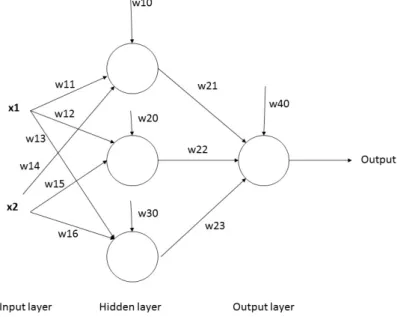
Figure 1: A basicANNstructure showing the different layers, inputs and weights
As seen in figure1 a basicANNis constructed by an input layer that receives an input x(n). These are then forwarded through weights w(ij), corresponding to each line which is multiplied with the input. The next layer is called the hidden layer were the weighted inputs are summated and introduced to a biased weight before being forwarded to the output layer. The output is
then compared to the expected output and the error is backpropagated layer by layer through the network. The weights are then adjusted accordingly. This is repeated until a satisfying result, or a pre-defined number of iterations, are achieved. One such iteration is called an epoch. After this is done theANNis trained and can be used to solve the problem at hand.
2.4.2 Convolutional Neural Network
AConvolutional Neural Network (CNN)is a feed-forwardANNwhose structure is inspired by the visual cortex in animals. Every neuron (or node) operates in a restricted space which is called a receptive field. Each of these receptive fields overlaps to a certain extent. Each nodes output can be approximated through convolution. TheCNN was designed to require as little pre-processing as possible.
In a CNN each neural is designed to process a small part of the input image which overlaps with the image parts next to it which is fed into another neuron. This operation allows for translation of the input image in the CNN. The network may contain layers of pooling, either local or global, which combines the outputs of the neurons and scales it down. It also includes fully connected layers as well as convolutional layers. The advantage ofCNNs is that they share weights across the convolutional layers. This makes it possible to detect the same feature across the entire image using the same pool of weights, also called a kernel. This minimizes the amount of memory that is required for the feature extraction. The pooling layers divides the input image into non-overlapping squares or rectangles. In every such geometry only the strongest response from a neuron is outputted if the max pooling is implemented. This reduces the spatial size of the representation. It is built on the assumption that the exact location of a feature is not as important as its relative location to other features. The pooling layer helps reduce the amount of parameters required in the network as well as the number of computations. Finally a fully connected layer is implemented to perform the main learning. The most commonly used activation function is the
Rectified Linear Units (RLU)since it is quite resistant to gradient vanishing effect that occurs in the backpropagation algorithm. During recent yearsCNN has shown substantial improvements over other state-of-the-art approaches in object recognition [5,6].
2.4.3 Recurrent Convolutional Neural Network
A Reccurent Convolutional Neural Network (RCNN) is implemented much like the CNN. The difference is that the convolution is performed a pre-defined number of times by the same filter. The result from each iteration will be convoluted again by another filter. After this all of the results are summated to the last feature map provided by the first function on the last iteration. This method allows for an increase in depth with just a few added weights.
2.4.4 Deep learning Deep Neural Network:
ADeep Neural Network (DNN)is very similar to theCNNin it also being a feed-forward network. It also contains convolutional and pooling in the hidden layers. However, theDNNoften contains more layers which allows it to achieve more complex functions because of its abstraction of input data [1]. A big difference is thatDNNsdoes not share weights between kernels but rather unique weights for each. This may increase the risk of overfitting as well as memory usage and computa-tional cost. TheDNNmay also contain normalization layers. Another big difference is that in a
DNNthere is no output layer but rather a classification layer.
Deep Convolutional Neural Network:
ADeep Convolutional Neural Network (DCNN)is a combination betweenDNNandCNN. It uti-lizes the strength of both as it contains both feature extraction and classification in itself [6]. It shares weights between kernels as theCNNbut with more layers and a classification in the output layer as inDNN. It has been shown that it can perform even better than theCNN, although with increasing calculation complexity as the depth and size of layers are increased [7]. An important thing to consider is that a deep network increases the risk of overfitting. This can be solved with
strategies such as dropout.
Reccurent Deep Convolutional Neural Network:
The Recurrent Deep Convolutional Neural Network (RDCNN) is essentially a DCNN with the same convolution steps as described in section2.4.3. This will allow for a deeper net with just a few added weights. The reccurence may increase the accuracy of the net but also increases the risk of overfitting due to the high level of abstraction of the input features [5].
2.4.5 Related work for optimization and FPGA implementations
There are multiple approaches to implementAIfor object recognition and it is important to look into what exists today. When it comes to implementations on a FPGA it is important to think of limitations as mentioned in section2.3.
Arunachalam Venkadesan et al. presents in their article [8] a solution to three major problems related to the limitations ofFPGAs. Firstly the computational complexity that is mainly driven by the non-linear activation function of aANN. The most popular non-linear function is the tan-sigmoid function which is defined as:
f (n) = e
n− e−n
en+ e−n
This equation induces a problem in hardware implementation. This is because it is an infinite series and to decrease the computational load it has to be truncated. This induces large truncation errors. If this is solved by Look-Up Tables (LUTs), these becomes large and any interpolation between values also becomes complex due to the fact that these combinations also is a power of e. Arunachalam Venkadesan et al. proposes a solution to this problem by implementing a different activation function called the Elliot function. The Elliot function is defined as
f (n) = n 1 + |n|
and contrary to the tan-sigmoid function it consists of only one adder and one divider. It is shown that the Elliot function performs as good as the tan-sigmoid function with less complexity and therefore faster execution in a benchmark test.
The second problem presented is the bit precision of the system. While a lower bit precision decreases cost and memory usage. This also decreases the accuracy of the system. Therefore, it is crucial to find the optimal precision to lower costs while maintaining an acceptable accuracy. The precision can be set by choosing, for example, an 8-bit signed or unsigned variable where the 4 most significant bits are the integer part and the 4 least significant bits represents the float part. This can be viewed in [9] where they receive an accuracy of 161 = 0.0625. Arunachalam et al. proposes a formula1 which helps them to find the precision Y2for variable A.
Y = A ∗ 2N Y1= wholepart(Y ) Y2= Y1∗ 2−N (1)
The final problem addressed is how to conserveFPGAutilization. Instead of implementing the entire architecture a multiplexing method is chosen and implemented. In the multiplexing method only the largest layer of theANNis implemented on theFPGA. This is then used in all the layers of the network. This is achieved by a controller unit that inputs the weights, inputs and biases corresponding to the layer that is currently being calculated. This method reduces resources used in theFPGA.
To minimize memory usage Ning Li et al. proposes in their work [3] an implementation that utilizes multiple computing engines to be able to optimize each computing engine to each different layer. All of the engines, or layers, were pipelined and this eliminated the need for a buffer to store the results, which serves as inputs to the next layer. This significally decreased memory usage and increased the parallelism. They found that a RCNN, along with a strategy called Global
summation, with the aforementioned computing engines lead to an implementation that would all fit on a single chip. This includes all of the computations from the start to the end. The implementation also performed two times faster than, at the time, the latest research. The global summation method used saved memory and DSP usage by not having fully connected layers. To pipeline all of the computing engines a FIFO-queue is implemented. This stores the results and forwards them to the next layer. The FIFO-queue makes it possible to calculate any large image as long as it has room for a sufficient amount of weights. Ning Li et al. compared their hardware with a CPU and found that their method were 380 times faster than the CPU and approximately two times faster than the latest research at the time. They achieved 409.62 Giga-operations per second and an accuracy of 94.5% and 98.4% on two separate datasets.
In [6] Byungik Ahn presents a CNN implemented on a FPGA that recognizes objects in a real-time video stream. By down-scaling the input stream and extracting image blocks it is able to classify more than 170,000 times per second and perform scale-invariant object recognition on a 60 frames-per-second video stream that has a resolution of 720x480. The system consists of theCNN
core, a pair of video encoder and decoder as well as pre-processing and post-processing modules. The down-scaling is done in seven steps in the pre-processing module where the size of the image blocks are halved in both x and y dimension every other scaling step. This will allow theCNNto classify objects at any scale. After classification the results are sent to the post-processing module which marks the classified objects with a colored frame. Byungik Ahn’s work uses only elementary components such as combinational logic, memories and arithmetic operators. This entails that neither main memory nor processor is used. A multi-category recognition is also implemented that enables the system to classify, or recognize, two different objects at the same time. This is done by using different weight sets in alternating frames. The more objects that is classified the more the recognition frame rate must be lowered. The connection weights are stored as 25-bit signed integers plus two exponent bits. These are used to bit-shift the product of large values in the connection weights effectively eliminating the need for floating-point operators.
Sajid Anwar et al. presents in [7] a fixed-pointDCNNwhich is optimized to reduce computation complexity and to speed up classification. This is achieved by quantizing pre-trained parameters from a high precision network through L2 error minimization layer by layer. The network is then retrained with the quantized weights. The results indicates that sparsity is achieved within the network. This reduces the amount of parameters and the memory usage by one tenth while obtaining better results than the high precision networks. By lowering floating-point precision to three and four-bit precision an 80% saving is achieved in hardware resources. By using the same input for each layer during the quantizing step a sensitivity analysis is performed on each layer except for the pooling layers, which are kept as high precision. This is done by keeping the other layers as high precision and computing the optimal weights one layer at a time. These weights are then added to the high-precision weights and compared to a validation set to find the optimal weights. Using this method a network that performs better, similar or comparable, while only using 10% of the memory that a high-precision network does, was obtained.
Ming Liang and Xiaolin Hu proposes in [5] aRCNNwhich performs static object recognition. The results obtained showed that their network performed better than state-of-the-artCNNs uti-lizing fewer parameters. TwoGPUswith data parallelism were used to run the experiments that were performed on four benchmark object classification datasets. The training was performed with the backpropagation through time algorithm [10] in combination with stochastic gradient descent. A regularizer is implemented through weight decay and dropout is used to minimize overfitting.
A 3DCNNis proposed by Daniel Maturana and Sebastian Schere in [11] called VoxNet. Voxnet differs from standardCNN by utilizing a 3D-point cloud, obtained through LiDAR, RGB-D and CAD data. Several authors have implemented RGB-D cameras in their work but instead of utilizing the entirety of the spatial data they just treat the depth as an additional input to their networks. This is called 2.5D networks. Daniel Maturana and Sebastian Schere utilizes a point cloud to find the spatial occupancy through a volumetric occupancy grid and predicts class labels through a 3D
CNN. The volumetric occupancy grid maintains a probalistic estimate of the environment through the use of random variables that corresponds to a voxel. This helps, from range measurements, in estimating free, occupant and unknown space. They implement their solutions on aGPUand their result shows improvements on state-of-the art results in various benchmarks while performing the classification in real-time.
2.4.6 Reasoning
There exists a lot of implementations ofANNsall with their own strengths and weaknesses. Since this thesis scope is to investigate the feasibility to implement real-time object recognition on a
FPGAthrough a video feed, it is natural to consider the limitations stated in2.3. TheFPGAwas also chosen over the GPUbecause of the latency, power-consumption and by request of Unibap. Keeping this in mind the method that is tested in this thesis will be aCNN. This is due to the fact of the weight sharing between convolutional layers, the fact that the classification is integrated in the network, the fact that it utilizes less resources than aDCNNas well as promising results. It is also the request of Unibap that this network is implemented. The focus will be in finding good configuration in terms of depth, kernel size, the amount of layers and which methods that is to be implemented. The implementation will also utilize the multiplexing method to conserve logic blocks and DSP’s.
3
Method
This thesis was proposed by Unibap and their request included a deep learning algorithm intended for use on aFPGA. An existing platform calledIVS-70is provided by Unibap. From this platform we can draw some requirements. With these in mind, research was performed on different deep learning algorithms and a choice was made as mentioned in section2.4.6. The next steps are to design the layout of the algorithm, decide how to train the network as well as to decide on the implementation.
3.1
Layout
The layout of the networks will need to be decided upon to find an optimal solution. This will be performed through the program Tensorflow [12]. Different configurations with different size of the feature maps as well as number of nodes in the fully connected layer will be implemented, tested and evaluated. The resource and timing demands on each of these configurations with different sizes of the variables will be investigated. This will give an indication towards what configurations performs well and this will be used as a basis for the decision of what configuration that will be implemented on a2.3in the future.
3.1.1 Deep Convolutional Neural Network
Figure 2: Structure of aDCNNfrom [13] .
The process of aCNNconsists of two parts. In the first part the feature extraction is performed and consists of alternating convolution and pooling layers. The second part performs the classi-fication and recognition and this is done through dense layers. The structure of aDCNNcan be viewed in figure2. In the figure, the convolution layers are called C-layers and the pooling layers are called MP-layers while the dense layers can be viewed at the end of the network.
TheDCNNandCNN works on the principal of receptive fields. This means that a neuron in the network is only connected to a small region of the previous layer. In the first layer the raw image, that is used as input, is divided into small regions. In figure2 this region is set to be 5x5. The resulting square is then shifted across the image to produce the input for subsequent neurons. The variable that governs how far the region shifts is called stride and is set to 1 in the figure. Since the region used is 5x5 and the total size of the image is 32x32 a stride of 1 will produce 28x28
different regions as inputs to the first convolution layer. The depth of the first convolution layer, in other words the amount of feature maps used, may all detect different features such as blobs, colors or edges and also governs how big the output becomes. Each feature map shares weights across the entire input field but different feature maps utilizes different sets of weights. This is built on the assumption that if a neuron is able to detect features in one part of the picture it should also be useful in finding the same feature in another part of the image. The activation function most commonly used is theRLUand this is due to the fact that it increases the non-linear properties of the network while leaving the receptive fields in the convolutional layer unaltered. As described by Ning Li et al. in [3] when three images, RGB, are used as input the output of a convolutional layer and theRLUis given by the equations2and3where yi,j,k(l) is the output of layer l, i, j and k is the 3D-coordinate of the node, w(l−1,f )a,b,c is the weights of filter f which is applied at layer (l − 1) and a, b and c is the 3D-coordinates of the filter weight. Finally, before being passed on to the pooling layer theRLUfunction σ is applied, which can be seen in4, which produces the output of the layer. x(l)i,j,k=X a X b X c
w(l−1,f )a,b,c yi+a,j+b,k+c(l−1) + biasf (2)
y(l)i,j,k= σ(x(l)i,j,k) (3)
σ(x(l)i,j,k) = max(0, x(l)i,j,k) (4) After the initial convolutional layer which summates the activations from the three channels. The subsequent convolutional layers may utilize two dimensions instead of three. After the convo-lutional layer andRLUthe output is used as input to the pooling layer. The pooling layer can be done in multiple ways. The basic method of the pooling layer is to divide the input into squares or rectangles of equal size that does not overlap. In a max pooling layer the different nodes in the pre-defined area are compared and the strongest (highest) response is chosen to use. This reduces the size of the input and this can be used as a new input to the next convolutional layer. If a max pooling layer with a kernel of 2x2 is used on an input of size 10x10 then the resulting output to the next convolutional layer will be of size 5x5. Another method is the average pooling method that works much in the same way as the max pooling. The difference is that instead of using the strongest response, the average response is calculated and used.
At the end of the network a fully connected layer is implemented much the same way as in a classicANN. Its output can be calculated the same as well, through a matrix multiplication and a bias offset. The output of this layer is in the form of a vector. For example, if 6 classes are to be classified the output will have the form as shown in equation5where each number represent the degree it belongs to each class. The output from5 belongs to class 1 to a degree of 10%, class 2 20% and so on.
Output = [0.1, 0.2, 0.05, 0.7, 0.3, 0.0] (5) Since the matrix multiplication of this layer utilizes a lot of resources Ning Li et al. proposes in their work [3] a solution called global summation. It is based on the same technique as global average pooling. Instead of having a fully connected layer it requires the same amount of feature maps as classes wished to be detected. This entails that it requires less resources, since only accumulators need to be utilized, as well as a reduction in overfitting.
To reduce the risk of overfitting, since a smaller training set will be used, a technique called drop-out may be used. Dropout is performed by actively excluding nodes during training. Every node has the probability of (1 − p) to be excluded from training. If excluded, the node and all its connections are removed during training and then included again after training. The training may be performed, as withANN, throughGradient Descent (GD).
3.1.2 Reccurent Deep Convolutional Neural Network
ARDCNNis implemented the same way as aDCNNwith a minor alteration in the convolutional layers. Instead of being convoluted one time in each layer the input is convoluted a pre-defined
Figure 3: Depiction of the reccurancy of aRDCNNfrom [3] .
number of times by the same filter F . The result from the convolution will then be convoluted again by another filter f and added to the next convolution by filter F . A depiction of the method, with three steps, can be viewed in figure3and the corresponding equations can be seen in equations
6,7 and8. It is based on the work of Ning Li et al. in [3].
Outputt=0= F ∗ Input (6)
Outputt=1= f ∗ (F ∗ Input) + F ∗ Input (7)
Outputt=2= f ∗ (f ∗ (F ∗ Input) + F ∗ Input)) + F ∗ Input (8)
3.2
Training
To achieve low error rates, it is recommended that a CNN is trained on a massive database of images. This is very time consuming and therefore two approaches will be tested and evaluated in this thesis. Firstly, a network that has been trained on a big database, such as the ImageNet database [14], will be implemented. The end-product that Unibap works towards will be working in simplified surroundings where the objects will be more easily recognized. This is why the second implementation will train on a small data-set and be evaluated to see if it is feasible to minimize the training. These two methods will then be compared and analyzed.
3.2.1 Backpropagation - Fully connected layers
To train theDCNNthere are a few different steps depending on which layer that is being trained. In the fully connected layer the backpropagation method is implemented. First the error, or cost function denoted E(yL), at the output layer needs to be calculated. This is done by the
squared-error loss function. The squared-squared-error loss function can be viewed in9.
EN =1 2 N X n=1 c X k=1 (targetnk− y n k) 2 (9)
where N is the number of training examples, c is the number of classes supposed to be identified, targetn
k is the n:th training example target of class k, and ykn is the actual output from the last
layer for training example n’s belonging to class k. Since the squared-error loss function is just a sum of individual errors across the training dataset this can be simplified to a single training example. This can be viewed in equation10.
E(yL) =1 2 c X k (targetk− yk)2 (10)
The partial from the output layer is simple the derivative of the error function and this can be seen in equation11. δE δyL i = d dyL i E(yL) (11)
After this is done the partial derivative of error, commonly known as deltas, needs to be calculated for each input to the current neuron. This can be viewed in equation12
δE δxl j = σ0(xlj) δE δyl j (12) where δxδEl j
is the delta for input xl
j to the current neuron. This is done for all neurons. When
this is done the errors at the previous layer needs to be calculated, in other words the error is backpropagated. This is done by equation13
δE δyil−1 =
X
wijl−1δE
δxlj (13)
where wl−1ij is the weight connected to the input xl
j in the next layer. Equation 12and 13is
then repeated through all fully connected layers in the network until the input to the first fully connected layer is reached. After this you have the gradients to all of the weights in the fully connected part of the network. This gradient is then multiplied with the negative learning rate and this is added to each corresponding weight and thus the higher reasoning, or dense layers, of the network has trained on one training example. The equation14 shows the variable which is added to the weights
∆wl−1ij = −η δE
δyil−1 (14)
where η is the learning rate.
3.2.2 Backpropagation - Max pooling layers
Since the max pooling layers does not actually performs any calculation but rather picks the neuron in the layer before with the highest activation it does not perform any learning at all. This means that the error is simply forwarded to the place where the highest activation is found.
3.2.3 Backpropagation - Convolutional layers
The backpropagation in the convolutional layers are different from the one performed in the fully connected layer. The error in the convolutional is known from the layers succeeding the convo-lutional layer. First, as in the fully connected layers, the gradients for each weight needs to be calculated for the current layer. To do this the chain rule is utilized and it must sum the contri-butions of all expressions where the variable occurs. Since the convolutional layer shares weights, every single xlij expression that includes the weight wab must be included. The equation can be
viewed in15. δE δwab = N −m X i=0 N −m X j=0 δE δxl ij δxlij δwab (15)
By looking at the forward pass of the algorithm mentioned in section 3.1.1 we already know that δxl ij δwab = y(i+a)(j+b)l−1 (16)
and therefore, get equation17.
δE δwab = N −m X i=0 N −m X j=0 δE δxl ij y(i+a)(j+b)l−1 (17)
In order to calculate the gradient, the value of δxδEl ij
must be known. This can be calculated by using the chain rule again as in18
δE δxl ij = δE δyl ij δyijl δxl ij = δE δyl ij δ δxl ij (σ(xlij)) = δE δyl ij σ0(xlij) (18)
Since we already know the error at the current layer the deltas can be calculated easily by taking the derivative of the activation function. The activation function, which is max(0, xl
ij), can
only give the answer one or zero except for when xl
ij = 0 when its derivative is undefined. After
this the error needs to be propagated back to the previous layer. Once again this is achieved by applying the chain rule as seen in equation19.
δE δyl−1ij = m−1 X a=0 m−1 X b=0 δE δxl (i−a)(j−b) δxl (i−a)(j−b) δyijl−1 = m−1 X a=0 m−1 X b=0 δE δxl (i−a)(j−b) wab (19)
Looking at this equation we can see that this is a convolution where wab have been flipped
along both axes. It is also important to note that this will not work for the top- and left-most values. It is therefore necessary to pad the top and the left with zeros.
Another thing to note is that when the convolutional layer closest to the input is trained. The equations needs to be expanded to three dimensions since three channels, RGB, are summated from the input.
3.2.4 Training data
Unibap wants to implement the work of this thesis in an industrial environment where it is supposed to recognize a small number of objects in a simplified environment. This will be targeted objects for different industries and therefore there exists no training data-sets for these objects. A training data-set will be created by taking pictures from different angles. The objects will then be digitally placed in different rotations and on different backgrounds. These images will then be utilized as the training data-set.
3.3
Implementation
The implementation, that will be done on aFPGA, will only contain the forward pass. This is due to the fact that it is more productive to train the network on an external hardware. This way the training can be sped up by utilizing server-parks or super-computers. After training the only part that will be needed on theFPGAfor recognition is the forward pass. This will be implemented and simulated for aFPGAand the results and timing will be analyzed and reported.
3.4
Analysis
The purpose of this work is to work on targeted objects in an industrial environment. One example is that the hardware might be fitted in an assembly line where this work would be used to identify a part which is packaged with identical parts. Therefore, it is not necessary to identify the object amongst different objects but rather make sure that just one of the objects is recognized. This entails that there will be no previous results to compare to. Instead the analysis will focus on the usefulness the work in this thesis will have in its intended environments.
4
Hardware
The platform intended is provided by Unibap and is namedIVS-70[15]. TheIVS-70is fitted with two cameras and has stereovision. Through disparity mapping it has the ability to see the depth, or distance, to the objects it sees. By always situating the camera at the same distance from the plane the objects are placed on all of the objects meant for detection will always be at the same distance. Because of this all of the objects will always be the same size and the work in this thesis does not have to implement any kind of scale-invariance. TheIVS-70includes both aGPU,Central Processing Unit (CPU)and aFPGA.
4.1
Cameras
TheIVS-70 is fitted with two Color or monochrome 5.2 megapixel camera lenses. They have a resolution of 2560x2048. The framerate is up to 25 frames per second when utiizing the full 5.2 megapixel and up to 50 frames per second when utilizing 1 megapixel. They have a global shutter with programmable exposure time.
4.2
Field Programmable Gate Array
TheFPGAin theIVS-70is a smartfusion2M2S050T [16] with a 166MHz ARM Cortex-M3 proces-sor. Its logic elements consist of 4LUTs and one DFF. There are a total of 56,340 of these logic elements. It also contains 72 math blocks which is used in multiplications. The multiplications can be performed on 17x17 unsigned variables or on 18x18 signed variables. The smartfusion2 contains a total of 1,314 kbit of RAM memory.
4.3
System on Chip
On theIVS-70there is aSystem On Chip (SOC)that has both aCPUand aGPU integrated on one chip. This chip is the AMD G-series GX-415SOC[17].
The CPU in the the SOC has 4 cores and works at a frequency of 1.5GHz while the GPU
5
Implementation
5.1
Testing
During the testing phase, to figure out which configurations works best, the program Tensorflow was used [12] and two tests were performed. The first test was performed on the MNIST database [18] and the second test were performed on a custom created database.
5.1.1 MNIST
The MNIST database is a database of handwritten digits. It has a training set containing 60,000 examples and a test set containing 10,000 examples. It consists of size-normalized and centered images taken from the NIST database. The pictures were normalized to fit in a 20x20 pixel box and later centeralized in a 28x28 image. This was done by computing the center of mass of the pixels and translating it to the center of the 28x28 image. This is the only size that was tested on the MNIST. Some examples of the images in the MNIST database can be viewed in fig4.
Figure 4: An example of MNIST images from [12] .
5.1.2 Custom database
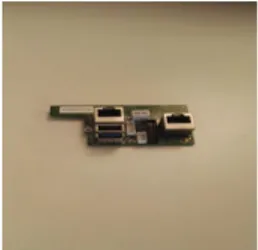
The custom database consists of images depicting different components in the IVS-70 taken on a white background from different angles. An example of images from the custom database can be viewed in fig5. The custom database contains 7192 images and the test were performed by leave-one-out method. This means that a random set of the images are used as validation and this set interchanges each epoch. The tests were also performed on 3 different image sizes, namely 28x28, 56x56 and 112x112. The tests were then compared by validating them on 1000 images.
5.1.3 Test setup
To get an idea of what the optimal configuration is four test setups were investigated. All the test involved two convolutional layers and one fully connected layer. This is due to the good performance on the MNIST database and this was used as a comparison to the custom database. The MNIST database was tested on 2D gray-scale images while the custom database was tested on 3D RGB color images. In test one the first convolutional layer has 32 feature-maps in the first
(a) Example one from custom database (b) Example two from custom database
Figure 5: Two images from the custom database
Table 1: Test results
Test Results (%)
Images MNIST Custom 28x28 Custom 56x56 Custom 112x112 Test one 98.96 93.1 74.2 86.3 Test two 99.32 95.4 78.1 88.8 Test three 99.2 91.8 88.9 86.7 Test four 99 92,6 91.8 84.2
convolutional layer and 64 feature maps in the second. The fully connected layer is built with 1024 nodes. In test two the first convolutional layer consists of 16 feature maps and the second of 32 feature maps. The fully connected layer consists of 512 nodes. In test three and four the convolutional layers are the same as in test two but the fully connected layer consists of 300 and 100 nodes respectively. Every test was performed with 10,000 iterations and the results of the tests can be viewed in table1.
As can be seen by the results both the MNIST and the custom database performs best on test two. And in case of the custom database on the size of 28x28. It should be noted that an increase of training images and more iterations might improve the results on the custom database. It also shows that the MNIST database is slightly better than the custom database. This might be because of the substantially smaller size of the custom database. The results shows that the custom database has acceptable accuracy for its intended use and therefore the expansion of the database is left for future work.
5.2
FPGA
implementation
During the course of this project Unibap notified that a proper database is to be provided although late in the project. This lead to the decision to implement the core modules of the network and verify its functonality so that a network of any size can be constructed. Because of this a presentation of all the test setups will be presented in regards to resources required as well as timing.
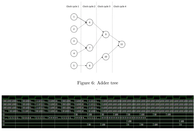
The first module is the multiplication and adder module. The multiplications in the network are pretty straight forward and since there are 72 math blocks on theIVS-70this limits the amount of multiplications per clock-cycle to 72. There is a small problem with the adder modules. Since the addition blocks on theFPGAare only able to take two inputs this leads to a problem in time. For example if there is 5 inputs that needs to be added this will take 3 clock-cycles. This can be viewed in6. This is not the case in the multiplication and adder module which only adds a biased to the result of the multiplication. This problem arises after the module where all the results from the kernel needs to be added together.
Because of this the additions in the network will be pipelined. This means that the first five values to be added are inputed into the adder tree, visible in fig6, at cycle one. On clock-cycle two these will be inputted into the next level of the adder-tree. At the same time the next 5 values to be added are inputted into the first level. Even though the first 5 values to be added
Figure 6: Adder tree .
Figure 7: Timing of module .
will take 3 clock-cycles the subsequent addition will only take one extra clock-cycle. This means that dataset n will take 2 + n clock-cycles to compute.
The next two modules are simple. Since the activation function used is the RLU a simple comparison block is utilized to achieve this. The maxpooling is simply comparing four values, but only two each clock-cycle, and outputting the highest and this can also be done with one comparison block. Both of these modules are one clock-cycle modules.
One decision made to simplify the first part of the network, the convolutional layers, theRLU
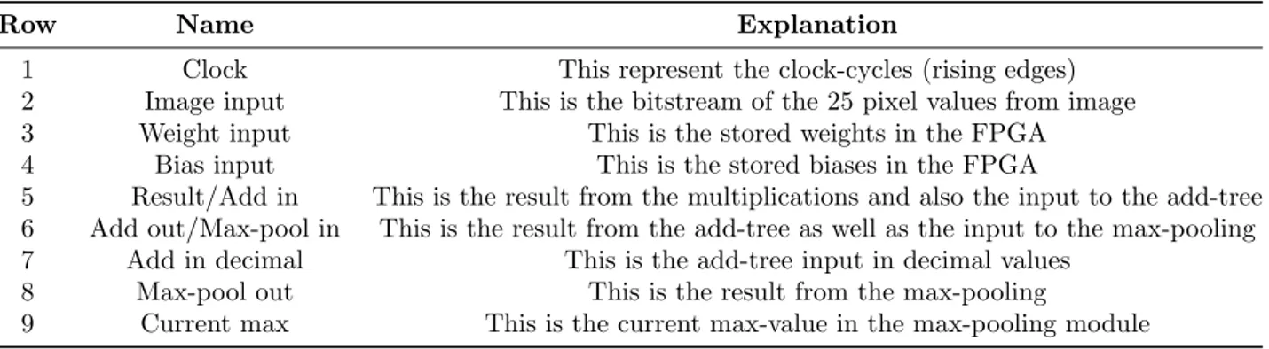
and the max-pooling, was to implement a specific module that works on a per kernel basis. This means that theFPGAwill not be used to its full potential during this stage since the kernels chosen is 5x5 in size. This means that only two of these modules may be implemented simultaneously since three of them will use 75 math blocks and this is not possible on the currentFPGA. These modules will input the first four nodes, namely the ones relevant to the first max-pooling, via a bit-sequence. This entails that the bit values from the image won’t be sent in left to right, but rather via the same squares dictated by the max-pooling function. An example of this module, running fully through from kernel via the add-tree andRLUto max-pooling and outputting the values of two such passes, may be viewed in figure7 where the explanations of each row may be viewed in table2. In this example the values are stored in 4-bit signed integers.
As visible in the figure it is clear that the first pass, from inputs from four different kernels to max-pooling output, takes 9 clock-cycles. However, the second output from the second pass only takes 4 clock-cycles. This indicates that the pipelining is working. This figure also confirms that the correct results are achieved from the multiplication, the add-tree as well as the max-pooling. In the first cycle the bitstreams in rows 2,3 and 4 indicate that the first 4 bits in the three bit-streams that represents the pixel-values in the image, the weights and the biases all have the bit-value of 0001 or 1 in decimal. This is repeated for all 25 positions in the kernel for simplicity. In row 4 and 7 we can se that the result of the multiplication with the added bias is 2 for all the positions. This can be verified by 1 ∗ 1 + 1 = 2. In the next cycle we can se the beginning of the pipelining where the next kernel inputs are calculated and forwarded to the add-tree with the result of 6 which can be verified in the same manner. Since the add-tree needs to add 25 values together it is known
Table 2: Row explanations
Row Name Explanation
1 Clock This represent the clock-cycles (rising edges) 2 Image input This is the bitstream of the 25 pixel values from image 3 Weight input This is the stored weights in the FPGA 4 Bias input This is the stored biases in the FPGA
5 Result/Add in This is the result from the multiplications and also the input to the add-tree 6 Add out/Max-pool in This is the result from the add-tree as well as the input to the max-pooling 7 Add in decimal This is the add-tree input in decimal values
8 Max-pool out This is the result from the max-pooling
9 Current max This is the current max-value in the max-pooling module
that the first layer of the add-tree will consist of 12 additions plus one odd value that needs to be pipelined along with the rest of the tree to achieve optimal timing. This means that 4 clock-cycles is needed to complete all of the additions. As depicted by the figure, four cycles after receiving the first results it puts out the value of 50. This can be verified by 2 ∗ 25 = 50 and this shows that the result obtained is correct. Furthermore it is also visible that the subsequent calculations only takes one clock-cycle and this verifies that the pipelining works as intended. In the bottom row the current maximum in the max-pooling module is displayed. It is clearly showing that the largest value obtained from the 4 positions in the image,150, is replacing the lower value of 50 and outputting this value after 9 clock-cycles as indicated by row 8.
5.2.1 Resources
The resources utilized by this implementation is described for test two on the custom database with an image resolution of 28x28 and will be shown for the other test setups. It is wort mentioning that the software utilized in the tests, Tensorflow [12], only works on 32-bit float values. TheFPGAon the other hand performs all of the multiplications on 18 bit values regardless of size specified on the values. This implies that the most optimal size of the values is 17-bit signed integers. These values are intended as fixed-point integers where the 6 least significant bits represents the float part of the value. This will not change the mathematics in theFPGA.
As mentioned in section5.1.3test two has a configuration where the first convolutional layer has 16 feature maps. This means that this layer needs to have 25∗16 weights. However since the netwok handles 3D images this needs to be multiplied by three giving us 1200 values required. It also needs as many biases as feature-maps which sums up to 1216. TheRLUand the maxpooling does not require any memory but after this is done the new image values, which is now 14 ∗ 14 = 196, needs to be stored. This means that 196 ∗ 16 = 3136 values are required. Going by the same principle, except that the input is now in 2D, the next convolutional layer, which have 32 feature maps, requires 25 ∗ 32 + 32 = 832 values. After the second convolutional layer the new image representations needs to be stored in 7 ∗ 7 ∗ 32 = 1568 values. For the fully connected layer the weights required can be calculated by equation20.
F C1 = SizeOf ImageV alues ∗ N rOf F eaturemaps ∗ N rOf N odes + N rOf N odes F C2 = N rOf N odes ∗ N rOf Outputs + N rOf Outputs
N rOf V aluesRequired = F C1 + F C2
(20)
Since the custom database has 512 nodes and 4 outputs this would come to a total of 812132 values needed for the network. If all of these values were to be stored internally on the fpga by 17-bit signed integers this would require 14,618,376 bits or 14,618.376 kbit. As mentioned, the
FPGA only has 1,314 kbit of RAM memory and therefore this is not possible. A summary of resource requirements for all the tests can be viewed in table3.
5.2.2 Timing
The timing will be reported in the same way as resources, with test two being described and the rest presented. Since only two kernel modules may be implemented at the same time this gives an indication on the time needed. Since the image is 28x28 and there is three of them, RGB images, the modules will need to run 14 ∗ 3 ∗ 16 = 672 times. As described earlier this section the first pass through will take 9 clock-cycles while the subsequent passes will take 4 clock-cycles. This means that to get to the second convolutional layer 9 + (671 ∗ 4) = 2693 clock-cycles will pass. To get through the second convolutional layer the same principle can be applied with the difference that the pipelining may continue so every calculation will take 4 clock-cycles. This means that to reach the fully connected layer from convolutional layer two (7 ∗ 16 ∗ 32 ∗ 4 = 14, 336) clock-cycles is required. The fully connected layer will take one clock-cycle to calculate 72 multiplications. The amount of clock-cycles to calculate the initial values to the fully connected layers can be solved by equation21.
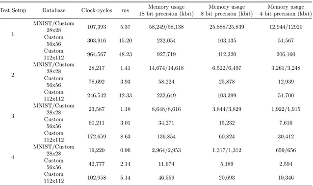
ClkInitial = ceil((F C1 − N rOf N odes)/72) (21) in this case this would amount to 11, 151 clock-cycles. During this the result to each node will need to be added together. That would mean that to each node 1568 values needs to be added. If this is pipelined then this would mean that the first addition will take 10 clock-cycles and the sub-sequent will take one clock-cycle each. This starts as soon as 1568 values have been calculated by the multiplication module. However, in this case that takes 22 clock-cycles which is a longer time than the addition takes. Because of this it is not necessary to pipeline the addition in this configuration. Instead the addition will be finished 10 clock-cycles after the last nodes inputs are calculated. The final calculation which is the output from the fully connected layer and the input to the classification layer consists of 512 ∗ 4 = 2048 multiplications. This requires 29 passes through the multiplication modules and luckily this can start before the 10 clock-cycles the last addition takes from the previous layer and those 10 cycles may be omitted from the total time. These 29 passes will take 29 clock-cycles. When 512 results are obtained which will be after 8 cycles the first add-tree may commence. One such add-tree takes 8 cycles as well. This entails that the last addition will finish 8 cycles after the last multiplication. Summating all of these cycles gives a total of 28,217 clock-cycles. Since theFPGAhas 20MHz as maximum clocking resource, which translates to 0.000050 ms per cycle, this would mean that one full forward pass through the network would take 1.41 ms. This translates roughly to 709 frames-per second which is way over what theIVS-70can muster. The rest of the tests can be viewed in table3.
Table 3: Test timing and resource demands
Test Setup Database Clock-cycles ms Memory usage
18 bit precision (kbit)
Memory usage 8 bit precision (kbit)
Memory usage 4 bit precision (kbit)
1 MNIST/Custom 28x28 107,393 5.37 58,249/58,138 25,888/25,839 12,944/12920 Custom 56x56 303,916 15.20 232,054 103,135 51,567 Custom 112x112 964,567 48.23 927,719 412,320 206,160 2 MNIST/Custom 28x28 28,217 1.41 14,674/14,618 6,522/6,497 3,261/3,248 Custom 56x56 78,692 3.93 58,224 25,878 12,939 Custom 112x112 246,542 12.33 232,649 103,399 51,700 3 MNIST/Custom 28x28 23,587 1.18 8,648/8,616 3,844/3,829 1,922/1,915 Custom 56x56 60,211 3.01 34,271 15,232 7,616 Custom 112x112 172,659 8.63 136,854 60,824 30,412 4 MNIST/Custom 28x28 19,220 0.96 2,964/2,953 1,317/1,312 659/656 Custom 56x56 42,777 2.14 11,674 5,189 2,594 Custom 112x112 102,958 5.14 46,559 20,693 10,346
6
results
This section describes the results of this thesis. Although the FPGA implementation was only simulated it verified that the network behaves as expected. The majority of the result can be viewed in the table in the previous section. The results leave a lot to be desired but unfortunately there was not enough time to explore all the possible solutions.
6.1
General research problem
What methods are feasible when implementing object recognition on aFPGAand which of these methods are the most suitable?
6.1.1 Question 1
The first question formulated was what limitations does the FPGA entail? It is quite clear that when working with theIVS-70the major obstacles are the amount of multiplication blocks as well as the size of the internal memory. Furthermore, the limitation in the size of the variables in theFPGAwill probably lead to a loss in accuracy. Otherwise it would seem asFPGAsis suitable for this purpose.
6.1.2 Question 2
Regarding the second question which is formulated as Considering the limitations in q1. what type ofANNis suitable? It was quite early on that both the research in itself as well as indications from Unibap indicated that aCNNwould be quite suitable. This is due to the fact of resource sharing as well as the accuracy proven in other works. There are however a few different methods explained in section2that were not properly investigated.
6.1.3 Question 3
Question three which is formulated Is it possible to fit the entire network on theFPGA? was investigated and the answer is yes it is quite possible to fit an entire network on aFPGA.
There are however some strong limitations on the network, especially on theIVS-70. The network is quite small and restricted in both image dimensions, layer size, depth and variable size.
7
Discussions
This section discusses the results of this thesis with some extra care taken to the questions formu-lated in the beginning.
Firstly, It should be pointed out that a lot of time in this thesis were used to learn language and programs pertaining to the specific hardware that was supplied by Unibap. Because of this the testing phase suffered in the way of less time for training and simulating. The decision to simulate the hardware implementation instead of synthetizing were taken to make sure that at least an accurate result, in regard to the simulation performed, could be achieved. In the beginning, it was decided that the network would focus on accuracy on a major database. But after discussions with Unibap it was instead decided that a custom database would be tested as well. This further diminished the time for testing since quite some time were put into creating the database. A while into the work Unibap announced that they would create a database that this thesis should include. It was later discovered that this database would not be ready until the very end and therefore the custom database included in this thesis is not as extensive as it should be. The results of this thesis leave a lot to be desired but it does however lay a solid base for future work.
7.1
Question 1
Even though theFPGAthat exists in theIVS-70brings a lot of restrictions to the network Unibap is working on upgrading their hardware to a largerFPGAwhich could allow the network to expand to larger dimensions. This is one of the reasons that test on networks that does not fit on the current hardware is included in this thesis. The results may be moot as of today but in the near future it will be relevant for the new hardware that is to be acquired. The new hardware will have more internal memory and more mathematical blocks and further testing of network configurations will be necessary to find the most suitable one.
7.2
Question 2
The decision to implement aCNNis something that would stand even after the hardware update. There are however some methods that could be relevant to test which might improve accuracy and lessen the resources necessary. Especially the global summation method that is mentioned in section3. There also exist a lot of other networks that, for time restrictions, were never explored. This is something that would have been very relevant to this thesis but to explore them all is impossible in the timeframe of this work. Another method that would be interesting to explore is theRCNNas well as the average pooling technique that both were omitted, also because of the lack of time.
7.3
Question 3
This is a very interesting part of this work. It is shown in section5.2.1that an entire network can fit on a FPGA. This is however a very small network that could be bigger if a betterFPGA is utilized. There are probably quite a lot of optimizations that could be done since the author of this work is relatively new to the language of verilog and many concepts pertaining to the coding of
FPGAs. However, the result shows that it is possible and with someone more experienced perhaps both the time and the resource demands may be diminished.
8
Future Work
As mentioned before the main thing to consider in future work is to implement and try different methods than the ones included in this work. There are so many unexplored method like the global summation method and recurrency in CNNs. Furthermore, testing different learning algorithms would be an expected part of the future work. All of the tests in this work is built on the backprop-agation method with a learning step of 0.01 through 10,000 iterations. It would be important to try different learning steps, number of iterations and algorithms. It would be especially important to investigate the backpropagation through time algorithm since this work is intended for a live video stream in the end. There are also completely different networks that was never considered for this work to try. Just to mention a few there are Deep-belief networks, Neural history compressor and Deep Boltzmann machines.
Another important part of future work would be to syntethize the network on a FPGA and actually confirming that everything works as intended. Not to mention doing a deep study of optimization inFPGAprogramming. There is a lot of improvements to be made after the upgrade of hardware that includes testing different configurations of the method investigated in this work since it only lays the foundation for bigger networks.
The custom database that is included in this work is something else that could be improved in the future. There is a whole area of filtering, composition, number of images required to explore. Even though Unibap is currently working on producing such a database some background work and tests could be included in future work. Another thing to consider for future work is the comparison between aGPUand aFPGA. This was intended to be in this work but since GPUprogramming is new to the author the decision to leave this for future work was taken.
Unibap started two similar thesis collaborations were this was the first one. The second one is more concentrated on accuracy than this work. Therefore, a merger of the two works would be something to consider for future work since this is the desire of Unibap.
9
conclusion
The focus of this work was to investigate and find the answer to the following questions. What methods are feasible when implementing object recognition on aFPGAand which of these methods are the most suitable?,What limitations does theFPGAentail?,Considering the limitations mentioned in question 1. what type ofANNis suitable? and Is it possi-ble to fit the entire network on theFPGA?. This work mainly focused on finding a suitable method forFPGAimplementation which could be applied in industry of today. This application could increase the productivity and speed of, for example, assembly. This would, according to Unibap’s beliefs, revolutionize industry of today. However, because of time constraints a lot of methods were bypassed without further investigation. It was however decided in tandem with Uni-bap on a certain network and configurations for this network were tested with acceptable results. It was discovered that theCNNis suitable forFPGAimplementation due to its resource sharing and accuracy. This network was implemented in a simple way on aFPGAwhich showed that it is possible to implement the network on the hardware.
It was discovered that the method presented in this work has acceptable accuracy for the intended use and that the network could indeed fit entirely on aFPGA. It was also discovered that this network would be severely restricted in its configuration but this could be improved when an impending hardware update is realized.
A custom database was created which showed promising results which could mean that a company interested in the end-product may easily be able to create smaller databases for their specific use with acceptable results.
There was also discovered that a hugh part of the area is still unexplored and that a lot of research could be done to improve the quality of this work amongst other things a more experienced
10
Acknowledgments
I would like to thank my supervisors Ning Xiong and Lars Asplund for the help with ideas and their continous support. Quick to answer any questions and a genuine interest in this work.
I would also like to thank the co-workers at Unibap who has helped me with areas they specialize in.
References
[1] Y. Kaneko and K. Yada, “A deep learning approach for the prediction of retail store sales,” in 2016 IEEE 16th International Conference on Data Mining Workshops (ICDMW), Dec 2016, pp. 531–537.
[2] Unibap, “Unibap homepage,” 2017, [Online; accessed 24-January-2017]. [Online]. Available:
https://www.unibap.com/
[3] N. Li, S. Takaki, Y. Tomiokay, and H. Kitazawa, “A multistage dataflow implementation of a deep convolutional neural network based on fpga for high-speed object recognition,” in 2016 IEEE Southwest Symposium on Image Analysis and Interpretation (SSIAI), March 2016, pp. 165–168.
[4] T. Cheng, P. Wen, and Y. Li, “Research status of artificial neural network and its application assumption in aviation,” in 2016 12th International Conference on Computational Intelligence and Security (CIS), Dec 2016, pp. 407–410.
[5] M. Liang and X. Hu, “Recurrent convolutional neural network for object recognition,” in 2015 IEEE Conference on Computer Vision and Pattern Recognition (CVPR), June 2015, pp. 3367–3375.
[6] B. Ahn, “Real-time video object recognition using convolutional neural network,” in 2015 International Joint Conference on Neural Networks (IJCNN), July 2015, pp. 1–7.
[7] S. Anwar, K. Hwang, and W. Sung, “Fixed point optimization of deep convolutional neural networks for object recognition,” in 2015 IEEE International Conference on Acoustics, Speech and Signal Processing (ICASSP), April 2015, pp. 1131–1135.
[8] A. Venkadesan, S. Himavathi, K. Sedhuraman, and A. Muthuramalingam, “Design and field programmable gate array implementation of cascade neural network based flux estimator for speed estimation in induction motor drives,” IET Electric Power Applications, vol. 11, no. 1, pp. 121–131, 2017.
[9] S. Li, K. Choi, and Y. Lee, “Artificial neural network implementation in fpga: A case study,” in 2016 International SoC Design Conference (ISOCC), 2016, pp. 297–298.
[10] J. Mazumdar and R. G. Harley, “Recurrent neural networks trained with backpropagation through time algorithm to estimate nonlinear load harmonic currents,” IEEE Transactions on Industrial Electronics, vol. 55, no. 9, pp. 3484–3491, Sept 2008.
[11] D. Maturana and S. Scherer, “Voxnet: A 3d convolutional neural network for real-time object recognition,” in 2015 IEEE/RSJ International Conference on Intelligent Robots and Systems (IROS), Sept 2015, pp. 922–928.
[12] “Tensorflow homepage,” 2017, [Online; accessed 24-January-2017]. [Online]. Available:
https://www.tensorflow.org/
[13] P. Bezak, Y. R. Nikitin, and P. Bozek, “Robotic grasping system using convolutional neural networks,” American Journal of Mechanical Engineering, vol. 2, no. 7, pp. 216–218, Oct 2014. [Online]. Available: http://pubs.sciepub.com/ajme/2/7/9
[14] S. U. Stanford Vision Lab, “Imagenet homepage,” 2016, [Online; accessed 24-January-2017]. [Online]. Available: http://image-net.org/
[15] Intelligent Vision System IVS-70, Unibap, January 2016, rev: 0.19.
[16] Microsemi, “Smartfusion2 soc fpga family,” 2017, [Online; accessed 24-January-2017]. [Online]. Available: https://www.microsemi.com/products/fpga-soc/soc-fpga/smartfusion2
[17] AMD, “1st and 2nd generation amd embedded g-series system-on-chip (soc),” 2015, [Online; accessed 24-January-2017]. [Online]. Available: https://www.amd.com/Documents/ AMDGSeriesSOCProductBrief.pdf
[18] C. J. B. Yann LeCun, Corinna Cortes, “The mnist database,” [Online; accessed 24-January-2017]. [Online]. Available: http://yann.lecun.com/exdb/mnist/