Adsorption of sulphur dioxide on spent shale in packed beds

T1998

KRlHO Tf EKKES LIBRARY CO LORADO SCHOOL of MINEfc

GOLDEN. COLO RADO 804QI

Adsorption of Sulfur Dioxide on Spent Shale in Packed Beds

by

All rights reserved INFORMATION TO ALL USERS

The qu ality of this repro d u ctio n is d e p e n d e n t upon the q u ality of the copy subm itted. In the unlikely e v e n t that the a u th o r did not send a c o m p le te m anuscript and there are missing pages, these will be note d . Also, if m aterial had to be rem oved,

a n o te will in d ica te the deletion.

uest

ProQuest 10782148

Published by ProQuest LLC(2018). C op yrig ht of the Dissertation is held by the Author. All rights reserved.

This work is protected against unauthorized copying under Title 17, United States C o d e M icroform Edition © ProQuest LLC.

ProQuest LLC.

789 East Eisenhower Parkway P.O. Box 1346

T1998

A Thesis submitted to the Faculty and the Board of Trustees of the Colorado School of Mines in partial ful­

fillment of the requirements for the degree of Master of Science (Chemical and Petroleum-Refining Engineering).

signed: Muhammad A. Hasanain Golden, Colorado Date: * 1977 ' CoI£>RAd£ J%INES Anthony IV.Hines Thesis S^dpisor PY Fi Dickson Head of Department Golden, Colorado Date; H/ir,. -f, / y £ , 1977

T-Ly^S

ABSTRACT

This investigation was undertaken in order to study the adsorption of sulfur dioxide on spent shale which was retorted for two hours and at a temperature of 700°C. An apparatus for oil shale retorting and the adsorption study was designed and constructed. The adsorbent was selected from samples of spent shale which were retorted at temperatures ranging from 300°C to 1000°C for retorting periods of 2 hours, 5 hours, and 15 hours. The primary objectives were to determine the effects of retort­ ing temperature and time on the adsorption properties of spent shale. Adsorption studies were conducted on the material which was retorted for two hours. Sulfur dioxide concentrations con­

sidered were 993, 1999, 2999, 4998, 7226, and 9704 PPM SC> 2 in ~ ^ 7 and adsorption temperatures were 10 °C, 27 °C, and 40 °C. The experimental breakthrough curves were fitted to theoretical plots derived by Antonson ( ) using an intraparticle diffusion model. From the curve fits of breakthrough curves, intraparticle diffu- sivities were calculated at two different temperatures. The equilibrium isotherms were fitted to Langmuir, Freundlich and Polanyi and Dubinin types of equilibrium isotherms. The heat of

-3 gm SC> 2 adsorption was estimated at a loading of 3.5 x 10 — =-- ■— .

cm solid It was found to equal 4.918 Kcal/mole. Finally the activation energy was estimated from the Arrhenius plots for three differ­ ent concentrations.

ABSTRACT iii

LIST OF FIGURES v

LIST OF TABLES vii

ACKNOWLEDGMENTS viii

INTRODUCTION 1

THEORY 5

Equilibrium Isotherms 5

Heat of Adsorption 9

Mass Transfer Mechanisms 10

EQUIPMENT AND PROCEDURE 14

Adsorbent preparation 14

Adsorption equipment 16

Experimental procedure 19

RESULTS AND DISCUSSION 20

Sample selection 20

Effect temperature & concentration ^2 on breakthrough curves

Equilibrium isotherms 32

Heat of adsorption 55

Intraparticle diffusion coefficients 55

Activation energy 69

CONCLUSION AND RECOMMENDATIONS 71

NOMENCLATURE 73

LIST OF REFERENCES 75

APPENDIX "A" - Experimental Data 79 APPENDIX "B" - Sample Calculations 88

T1998

LIST OF FIGURES

Page 1. Schematic of Oil Shale Retort 15

2. Gas Adsorption Apparatus 17

3. BET Surface Area Analysis 28

4. Adsorption of SO2 on Different Spent Shale 31 5. Experimental Breakthrough Curves

(993, 2999, and 7226 PPM) at 10°C

6. Experimental Breakthrough Curves -(1999, 4998, and 9704 PPM) at 10°C

7. Experimental Breakthrough Curves (993, 2999, and 7226 PPM) at 27°C 8. Experimental Breakthrough Curves

(1999, 4998, and 9704 PPM) at 27°C 9. Experimental Breakthrough Curves

(993, 2999, and 7226 PPM) at 40°C 10. Experimental Breakthrough Curves

(1999, 4998, and 9704 PPM) at 40°C 11. Experimental Breakthrough Curves

(10, 27, and 40°C) for 1999 PPM 12. Least Square Fit to Langmuir Model

(T=10°cf

13. Least Square Fit to Langmuir Model (T=27°C)

14. Least Square Fit to Langmuir Model (T=40°C)

16. Least Square Fit for Freundlich Model at 10 °C*

17. Least Square Fit for Freundlich Model at 27°C~

18. Least Square Fit for Freundlich Model at 4 0 °C

42 43 15. Equilibrium Data Fit to Langmuir Model 45 46 47 48 19. Ecruilibrium Data Fit to Freundlich Model 50

52 53 47 58 61 62 63 64 65 66 67 68 70 Least Square Fit for Dubinin Model

at 27°C

Least Square Fit for Dubinin Model at 40°C

Polanyi Model

Equilibrium Isosters

Curve Fit for 993 PPM at 103C Curve Fit for 2999 PPM at 10°C Curve Fit for 4998 PPM at 10 °C Curve Fit for 993 PPM at 4 0 °C Curve Fit for 1999 PPM at 40°C Curve Fit for 4998 PPM at 4 0 °C

Diffusion Coefficient, as a Function of Concentration at 10°C

Diffusion Coefficient as a Function of Concentration at 40°C

Arrhenius Plot

T1998

LIST OF TABLES

Page I. Chemical Analysis of Oil Shale Retorted for 2 Hours 21 II. Chemical Analysis of Oil Shale Retorted for 5 Hours 22 III. Chemical Analysis of Oil Shale Retorted for 15 Hours 23 IV. X-Ray Analysis of Oil Shale Retorted for 2 Hours 24 V. X-Ray Analysis of Oil Shale Retorted for 5 Hours 25 VI. X-Ray Analysis of Oil Shale Retorted for 15 Hours 26

VII. BET Surface Area Analysis 27

VIII. Adsorption of SO^ on Different Samples of Spent Shale 30 IX. Equilibrium Data and Langmuir Constants 44 XX. Equilibrium Data and Freundlich Constants 49 XI. Equilibrium Data and Dubinin Constants 54 XII. Equilibrium Data to Fit Polanyi Model 56

Acknowledgments

The author wishes to express his gratitude to Dr. Anthony L. Hines for his guidance in all aspects of this work. Appre­

ciation is also extended to Dr. R . Baldwin and Dr. E- Sloan for acting as committee members. Acknowledgments also go to Dr. John J. Duvall, Mr. Howard Jensen, and Dr. Richard E.

Poulson of the Laramie Energy Research Center for their support throughout the project. Also the support of the United States Energy Research and Development Administration under contract number E (29-2)-3780 is gratefully acknowledged. And last, but not least, the author wishes to gratefully acknowledge his

wife, Zaheiah, for her patience and good humor in the face of occasional adversity.

T1998 1

INTRODUCTION

There are two major processes used to produce oil from oil shale. One of the major processes is mining the shale and recovering the oil in an above-ground retorting facility. The other process is removing the oil from an underground

formation in an in situ process.

Above ground retorting processes, although studied ex­ tensively, suffer from a number of ecological problems asso­ ciated with the disposal of large quantities of spent shale. It has been estimated that the production of 250,000 barrels per day of shale oil will create more than 100 million tons of spent shale annually. Using the TOSCO II process and retorting 35 gal/ton shale, in which the spent shale was 81 weight per­ cent of the original unretorted shale, Striffler, Wymore and Berg (33) estimated that the spent shale from a 250,000 barrel/ day industry would cover an area of more than 44,000 acre feet annually.

The in situ approach, however, is perhaps the more attrac­ tive of the two major processes since the oil is extracted from the shale by heating the underground formation. This process eliminates mining the shale and the pollution problem that accompanies the disposal of spent shale.

In situ processing of oil shale is mainly based on the initiation of combustion or introduction of heat into the formation which results in the decomposition of kerogen into

bitumen, that is converted to oil, residual carbon, hydrocar­ bon gases, and combustion products. The relatively lower vis­

cosity oil, combustion gases, hydrocarbon vapors, and water produced during the process then flows horizontally through induced fractures and through the shale structure to surround­ ing wells where they are collected. The rate at which the burn front moves through the formation depends on a number of

factors, including shale porosity, diffusivity, permeability, oil content, and the rate of air injection.

For a sizeable shale oil reserve to be recovered, several fundamental questions must be answered, common to both in situ and above ground retorting processes. One of these questions is the adsorptive and absorptive properties of the spent shale and the transfer rates of gases flowing through the formation. It has been estimated {IX) that for a 50,000 barrel/day in situ process with no gas recirculation and with all the exhaust gas

flared and vented to the atmosphere that 70,714 tons per year of sulfur dioxide would be emitted. Assuming 75% gas recircu­ lation and cleaning the remaining 25% to a sulfur dioxide level of 500 PPM, the Colorado emission standard, 8406 tons per year of SO2 would still be emitted to the atmosphere. Recently it was noted that less SO2 than was expected was given off from the controlled state retort at Laramie and this was attributed to the uptake of S O2 by the oil shale.

In this work the adsorption of SO2 on spent shale was investigated. Breakthrough curves and equilibrium isotherms were obtained at three different temperatures and heat of

T1998 3 adsorption and diffusion coefficients were calculated- Spent shale samples were produced by retorting raw shale which was obtained from Laramie/ Wyoming. The particular material used contained 35 gallons of oil per ton of shale as found by

Fischer Assay.

In one investigation, spent shale samples from both above and below the Mahagony Marker were analyzed by

Culberston, Nevens, and Hillingshead (r) and samples from both zones contained more than 9% total residual carbon and large percentages of calcium, magnesium, and iron oxides. At re­ torting temperatures in the presence of water, the carbon that remains in the shale should be activated to some extent and should^provide an effective adsorbent for hydrocarbon and combustion gases. Upon considering the composition of the spent shale, the uptake of gases formed during retorting is quite plausible.

The removal of sulfur dioxide from a gas stream can be carried out by several different processes. For example, the

"chemico-basic" process uses a slurry of MgO to react with SC> 2 to form magnesium sulfate whereas in the limestone wet scrub­ bing process calcium sulfate is formed. A third process makes use of sodium salts to react with SO2 to form sodium sulfite/ bisulfite. Another method makes use of the activated carbon

that is produced from charred peanut hulls, as demonstrated by Hatfield,. Murphy, and Hines (/£) .

Spent shale from above ground facilities can be used as an adsorbent of SO2 from the process gas streams at a low cost

in industry. Also, the introduction of combustion gases into the underground formation where in situ processing has occured appears to be an effective method for disposing of waste gases.

T1998 ₅

THEORY

In this investigation, there are two types of information necessary to describe the unsteady state adsorption behavior resulting from the contact of a fluid containing an adsorbate and a solid adsorbent: 1) equilibrium relation between con­ centration of adsorbate in gas phase and the concentration of adsorbate within the particle, and 2) the mechanism governing the transfer of adsorbate from one phase to another must be known or estimated.

Equilibrium Isotherms

Equilibrium isotherms, which can be of several types in­ cluding 1) irreversible, 2) unfavorable, 3) linear and 4} favor able, have been modelled by many theoretical and semi-empirical equations. The equilibrium isotherm equations used in this

study are some of the most widely used. They are the Langmuir isotherm model, the Freundlich equation and the Polanyi poten­ tial model.

Langmuir Isotherm

The derivation is carried out by using a measure of the concentration of the gas adsorbed on the surface. The follow­ ing assumptions are used for the derivation:

1) All the surface of the solid has the same activity for adsorption.

3) All the adsorption occurs by the same mechanism/ and each adsorbent complex has the same structure.

4) The extent of adsorption is less than one complete mono- molecular layer on the surface.

In the system of solid surface and gas, the molecules of gas will be continually striking the surface and a fraction of these will adhere. Introducing the concept of an adsorbent concentration q*, expressed in moles per gram of solid, and Cm which represents the concentration corresponding to a com­ plete monomolecular layer on the solid, then the rate of ad­ sorption, moles/sec-gm solid is:

r = k C*(C - q*) Eq. (1)

a c m ^

where, ^ _ forward reaction constant c

C* ss adsorbate concentration. The rate of desorption is given by:

rd = kc q * E q * ^

where 1

9 k = reverse reaction rate constant c at equilibrium, r^ = r^ k' q* = k C*(C - q*) Eq. (3) C o m a.C* or q* = 1 + a "c* Eq> {4) k _ 2 where a. = r-r c 1 k m , c k and a^ = . 2 k ' c

T1998 ₇ Freundlich Isotherm

This isotherm equation is usually used over a small con centration range, and particularly for dilute solutions. The adsorption isotherms are described by an empirical expression usually attributed to Freundlich.

where q* is the apparent adsorption per unit weight of adsor­ bent, and K and n are constant. C* is the adsorbate concen­

tration.

Dubinin-Polanyi Isotherm

Dubinin (9) and his collaborators derived the isotherm equation using the potential theory originally formulated by Polanyi (26)- According to Polanyi's treatment, the "adsorption space" in the vicinity of a solid surface is characterized by a series of equipotential surfaces, surfaces of the same adsorp­ tion potential. When the volume between the two surfaces of a molecule is filled with adsorbate, the equilibrium pressure is P and the adsorption potential at the surface is obtained di­ rectly from the usual expression for chemical potential,

where Pq = saturated pressure of the adsorbate

AG = difference in free energy between adsorbed species and the corresponding saturated liquid at the same t emperature

q* = K[C*]V n Eq. (6)

AG (1 2 — a* RT In p Eq. U )

ijl ^2 ) = chemical potential of sorbed species

The basic postulate of Polanyi's theory is that, for a given system, the adsorption potential is independent of temperature and depends only on the filled volume of the adsorption space,

AG = f(W) , <-^ff)w = 0 Eq. (?) The volume W is given by

W = 2 s q . (£)

where x = adsorption in grams corresponding to pressure P p * fluid density.

A plot of AG vs W yields a "characteristic curve" which is in­ dependent of temperature.

Polanyi made no attempt to derive an expression for the adsorption isotherm from the potential theory, but Dubinin

( 9//C?) and his collaborators have developed such an expression. This was done by introducing an affinity coefficient, 3, where

AG,

3 = ^ Eq. (9)

Dubinin claimed that for two different vapors at the same

filling W of the adsorption space on a given solid, the adsorp­ tion potentials will bear a constant ratio to one another no matter what the actual value of W.

Now if adsorbate "2" is a vapor taJcen as an arbitrary standard, then Eq- (9) may be rewritten as,

3

- %

where the symbols with suffix zero refer to the standard vapor and those without a suffix to the other vapor.

T1998 9

The characteristic curve is defined in an alternative way for the standard vapor as,

W = f (ACJ Eq. (H )

upon inserting Eq- U O ) * Eq. (If ) becomes

W = f (AG/3) Eq. U l )

Dubinin advanced arguments favoring the view that the volume space may be expressed as a Gaussian function of the adsorption potential. For the standard vapor, this becomes

2

W = W o e _a AG° Eq. (13 )

where Wq = total volume of all micropores

a' = constant characterizing the pore size distribution By reference to Eq. (/<?) , Eq. U3 ) can be written as

W = W

e _a'

(AG/e)

Substitution for AG from Eq. ( ^ ) , Eq. {/if) becomes,

p

W = W 0 exp[- 2 L (2.303RT log10 ^ 0 3 Eq. (15)

3 or

P 0> 2

log10 W = 1Og10W 0 “ B(log10 “ P 5 E q ‘

Where B = 2.303 SI (RT)2

8 Heat of adsorption

The equilibrium data also yield values for the heat of adsorption. Hersh u ? ) has shown that at constant loading

AH H

8(InP)

3 (1/T) _a* Eq. U g )

plots of In P vs 1/T can be analyzed graphically for the slope at constant loading in order to obtain AH . A typical isoster

and the calculated value of heat of adsorption are described in the results section.

Mass Transfer Mechanisms

A differential material balance for the fluid phase is to be written before considering the transfer of adsorbate from

one phase to the next. The appropriate balance is

„ ac ac i ac- _ ,a c. _ az at m a t = DL < 7 ^ e^-8z Z n m - L da m - ' R - at • B

= bed bulk density PB = fluid density

z = bed void volume

The last term on the right side of Eq. (/9) accounts for axial diffusion. Acrivos (X) has used the equation in -this form,, although Rosen and most other authors have neglected it based on the assumption that the axial diffusion is small

dC

compared to the bulk transfer term (V ) . Using this assump* tion, Eq. (/^) can be reduced to

v ( ! § + + i (! ? > = 0 E *

-Eq. (£LQ) assumes a constant flow rate throughout the column which would be strictly true only for the case of an infinitely dilute solute. Since the system of interest was extremely dilute and incompressible, the equation given above does apply. The above equation can be further reduced if the following transformations are used

T1998 11

G = t - Z/V Eq. (21)

X = Z/mV Eq. cZT)

Eq. (.2/5) then becomes

■ — - - — Ecr (11)

ax “ as q '

The above equation shows the rate of adsorption as a function of the concentration changes along the bed length.

External mass transfer through the stagnant film surround­ ing the adsorbent particle may be represented by

If

C* = bulk adsorbate concentration

Cg = equilibrium concentration at solid surface.

Intraparticle diffusion for a homogeneous particle is given by

^ i 2 3 2 ^ i

_ _ _ DV2 q. = D ^ (r — -) Eq. (25) with initial and boundary conditions

IC I q i (r ,X, 9) = 0 at 9 = 0 0 < r < RQ Eq. (2.5-a)

BC I 0 = C/C0 = 0 at X = 0 t < 0 Eq. b) BC II 0 = C/C0 = 1 at X = 0 t > 0 Eq. (25-c) Assuming the diffusion rate is radialy dependent only, the over­

all average diffusion throughout the particle may be found by integrating over the particle volume

Eq. (13) was used as the starting point for the generation of diffusion controlled breakthrough curves for systems exhibiting Langmuir type isotherms.

Eq. (15) may be solved for constant surface concentrations to give the series solution

H(r,0)= J - l f i 1 2 sin(a r) e ' ^ 9

0 1 a=l . 11 Eq. (2-f)

where a = -2? n R

H(r,S) is the solution of the problem of solid diffusion into an initially empty spherical particle.

After applying Duhamel’s theorem to transform Eq. (2?) to the case of varying surface concentrations, the result is sub­ stituted into Eq. (26) . After interchanging the integration and summation so that the integration with respect to r may be carried out,

1 - % £ f q s e - DCTn (^ d X Eq. (ig) R n=l o-l

where X is a dummy variable of integration. Leibinitz’s rule for differentiating an integral may be employed to yield

CO

dc ac 6D

\f

55c ae ” 72 /] ax ^ 11 Eq. uf) K / O

n=l

Eq. (Z9) has only two unknowns, and to get the concentration profile, one should obtain an expression for q in terms of C

Rosen (27) evaluated q from Eq. (Z*j) and (25) to obtain s

T1998 ₁₃

In 1952 Rosen published an analytical solution to Eq. (2?)

assuming a linear isotherm. The generated breakthrough curves were used to calculate diffusion coefficients and external mass

transfer coefficients.

Rosen's basic approach was followed by Antonson (40 in obtaining theoretical curves valid for systems that could be represented by a Langmuir type of equilibrium isotherm. When q is eliminated from Eq. (J29) by use of the Langmuir isotherm,

and the resulting expression substituted into the fluid phase mass balance, expressed as Eq. iZ3) / the result is Eq. (31 ) .

ax = ~ ~ 2 2 - S a x h + a_C*^ expC-D(-g-) *(S-\)]dX

R n=1 0 2 Eq. (31 )

2n 3Da.

Defining </> - C/C , = - y 9 , *n = “y / Eq. (3f ) becomes mVR

1 £ . -2 T 9(^/(1+a2C*n c -l/2 n 2- 2 (9T -X)dX EC. C

3Z)

dr' a=i ax

The above equation was used as the starting point for solution by numerical methods. A computer program which duplicates Antonson’s numerical solution was used and values of C/Cq were

generated as a function of a and The use of the generated breakthrough curves in fitting experimental data is described

in the results section along with graphs of the computer or intouts.

EQUIPMENT AND PROCEDURE

Adsorbent Preparation

Samples of raw shale were obtained from Laramie, Wyoming, and the material used contained 35 gallons of oil per ton of shale as found by Fischer Assay. A large quantity of raw shale was ground and mixed several times so that the effects of retorting temperature would not be masked by variations in properties of raw shale- The samples were sieved and the shale which passed a one— fourth inch screen but were collected on a one—eight inch screen provided a homogeneous material for this study.

The retorting and production of spent shale was carried out in a 2 foot long stainless steel retort with an inside diameter of 2 inches. The retort as shown in figure 1, was sealed with threaded caps that had been tapped at each end to allow for the removal of oil and combustion gases and to

provide a means of controlling the atmosphere inside the retort. Oil shale was packed into the retort which was then

sealed and placed in a furnace. Nitrogen was passed through 3

the retort at a rate of 15 cm /min to provide an inert atmo­ sphere while retorting- The retort was then heated to the desired retorting temperature and then the samples were re­ torted for a fixed period of time. The retort was then cooled to ambient temperature while nitrogen continued to flow. As the processed samples were collected, they were crushed and

T1998

Schematic of Oil Shale Retort Figure (1)

V E N T

sieved to the desired size (20/40 US mesh). The samples then were analyzed for residual carbon, hydrogen, nitrogen, sulfur, and heat content. In addition, an X-ray diffraction analysis of each sample was conducted to determine the effects of re­ torting temperature on the mineral contents of the processed shale.

Adsorption Equipment

The experimental apparatus was designed and constructed to utilize an ultraviolet detector to measure and record gas concentrations. The apparatus, shown in figure 2, consisted of the following.

Constant temperature bath

A refrigeration-heating cycle water bath was used. The water temperature in the bath was automatically controlled to

desired temperature, and also it was checked from time to time by a regular thermometer to assure a constant temperature

during the 'experimental run. Heating coils

Heating coils were used to allow for the adsorbate to reach the desired temperature. Since the gas heat transfer

STU

coefficient is relatively low (in order of 50 — ~— ) ' a 60 ft

PT °p

long heating coil was used. The coil was made from a 1/8 in.. OD. stainless steel tube.

G a s A d s o r p t i o n A p p a r a t u s T1998 ₁₇

Sr

£2 V

V

C

O

N

S

T

A

N

T

T

t

h

p

C

R

f

t

T

M

R

O

B

M

H

Flow Meter

The gas flow rate was continuously monitored with a rota­ meter type of flow measuring devise which had been calibrated to experimental conditions. The calibration curve was obtained using a soap bubble flow meter and is given in Appendix C.

Because of the sensitivity of flow rates to adsorption data, flow rates were checked periodically with a soap bubble meter to insure steady flow conditions.

Ultraviolet detector

The effluent gas concentration was continuously monitored with a Beckman model 25 ultraviolet detector. A scan of the wavelength was performed from the visible to the ultraviolet region in order to obtain the highest wavelength peak. This was 198& which is in the ultraviolet region. The detector was hooked to a chart recorder which gave a constant chart speed that ranged from 0 . 1 in/min- 1 0 in/min.

Packed column

The column used in this study was prepared from a 1/2 in OD stainless steel tube 7.5 inches in length. It was furnished with union reducers at both ends to make it easy to be hooked

to one end of the heating coil and the other end to the UV detector. Packing the column to insure a constant amount of material for each run was considered to be an important part of the procedure. Each end of the column section contained a 1/4 in section of pyrex glass wool to prevent small particles of spent shale , from being carried away by the gas flow.

T1998

Experimental procedure

After the column was packed and placed in the constant temperature bath, pure nitrogen gas was passed through the packed bed to flush out any impurities and to establish a base line. The pure nitrogen gas was passed through the column until the bed and the gas reached thermal equilibrium. The gas flow rate of the SC^-nitrogen mixture was then started and the effluent gas concentration was continuously monitored and recorded- The sample gas was continued until the effluent

and inlet concentrations were equal. At the end of each run, the column was disassembled and a fresh sample was packed in the column for the next run.

RESULTS AND DISCUSSION

The results of the spent shale sample selection, effect of concentration and temperatures on the experimentally de­ rived breakthrough curves and isotherms., and the heat of adsorption calculated from equilibrium isotherms are pre­ sented in this section along with the computer generated breakthrough curves as fitted to the experimental ones.

Analysis of the experimental data yielded approximate values for the overall intraparticle diffusion coefficients.

Sample selection

Selection of spent shale on which to adsorb the gas was an important consideration because of the variation in shale properties found at different retorting temperatures and re­ torting times.

The chemical and X-ray diffraction analyses for all re­ torting times and temperatures are given in Tables I, II, III, IV, V, and VI. Also a BET surface area analysis was performed on samples which were retorted at temperatures ranging from 300°C to 1000°C for 2 hours. The results are given as a func­ tion of retorting temperature in table VII and are shown

graphically in figure 3.

Since it was noted that retorting temperature appears to more strongly influence the properties of the spent shale than does retorting time, material that had been retorted for two hours was used. The selection of the retorting temperature

Che mical Analyses of O i l S h a l e R e t o r t e d f o r T w o H o u r s T1998 21 B t u tn p as p P 03 -p - • « • 0 ♦ • • © p in o p in © pH p © 3 H o in in CO in p X © O a\ CN p CM p rH P 3 0 O CN 4J s a> o u a a* 4J cn P CD S © s »o o p u o © -r^ U Q U 3 IW r—4 3 CO s © cn$ o c © O 5-1 *U SH 3 o J3 U tQ u o o ttk D» © s u ■P 3 -U 4J (0 Q u u © © ai Cm £ © &« o P 3 S O p p m 0 CN P CN CN as J2 p in p CN © P 10 CN cn u • • • • • • • • U as O CJ p 3 3 cn p CN CN CN CN © O P O p r- O CO CO P o 00 © £5 CO o P Cl as 10 p p 3 P • * ♦ • * • • • P as 2 U p m in p P CN o o in © o p CD r* in 0 r- m p- CN P in p 0 • *• • • • ■ • ♦ 1 7 CO P 18 18 14 as *H © CN 10 CO o p r- p in 10 in p in m 0 0 • » • • # • • • O o o o o o o o CO 10 0 m CN p p p in in p p P p CN ip • • • •. • • • • o o o o O © o © CN p 0 n c\ CN CO «—4 P in p ip o P o O • • • m * » • • P o o o © © o o m p 0 p p p CN © p 0 tn CN cr> as o p • • • 0 ♦ 0 • • p as r*^ r* 0 P p © © o o © O o o © o © © © © © o o p p 0 0 t-* © as © p

Chem ic al Analyses of O i l S h a l e R e t o r t e d f o r F i v e H o u r s c 0) o u a 04 -U JZ -H 0 1 2 3 A 4J 4J (8 e <D 0 S 4J c o u o «H £ £ o to X2 £x w M (8 o u (8 C H O 0 X2 £ 5-t *H (Q s u 0 £ T3 O *H XI X M O 0 -H o a M 3 U4 f-4 3 cn £ 0 a o h 4-> £ 0 0 1 o *3 £ O xs h (8 O r- OX OX tn in GO r-VO r-4 OX in VO in o O O o o VO rH »h CS CN i—4 *—4 GO cn ox *—4 © vo CN OX VO r-» ox vo i-- r-• • • • • • • GO in »—4 pH r-4 r—4 o o vo CN rH VO m r- CN ax CN ox rp r- ■NT CN • • • • • • • • tn in CN H o O H CO vo ax i—4 ^3* r-4 i—4 rH CN CO ox O m r- CO • • • • • • • • 1 0 1 9 1 9 1 7 OX vo rH o r—4 r- vo vo ox ox T vo m •n* in in m in • • • • • * • • • o o o o o o o o o in CO VO vo m in VO in •Q* cn CN i—4 r-4 • • ♦ • • • • • o o o o o o O o cn rn GO TT ■ CN r* r-» CN CO o CN CN o o © • • m • • » • ■« H © © O © o o o CN ax r-4 CN VO ox OX rH VO ox 'ey VO o r-4 r-4 O • • • • • • • m o r- VO m i—4 rH a o tJ» 0 £ H •H 3 -P 4J 5-4 0 o s-» •P 0 0 04 OS £ 0 o O O o © o o o o O o o © o o m rr in vo r- 00 ox o rH

T1998 23 M M W ® rH 4 2 (0 eh CD U 3 o c (1) a) 4J M-i 5-1 O *3 0> -P U O 44 0) a: rH <0 x: LQ o m •H co >i rH (Q c < OS O •H e a jC o 44 c a> o Jh a> CU cn -r-4 0 3 44 0 4-5 44 CO C d) a> 0 4J c o u o •H £ £ o CO 43 O' U U CQ o a <0 c JH o <U 43 £ U -H CQ s o © £ TJ O *’H 42 X SH o CO hH u a u 3 MH rH 3 0 C a O U 44 c © cn o u TJ >4 C O 43 5h CO O vo VO r- Hp rH O in vo cn VO © GO © n* n* cn rH rH CN CN rH © VO CN rH n» rH © © CN © rH in cn © © © r- * © -H • • • • • • « £ vo CN rH rH © o © CN CO m cn CN HP © © CO rH cn c\ rH © CN © • • • • • • • • rp in in ■ cn © O © in CO o in © © © © vo © VO © n* © CN • • - • • • • • • r- CO © © rH cn o © rH rH rH rH rH CO rH in nr rH CN r<* © in in n* © © © HP • • • • • •. — • • o o O © o o © © vo o o cn CN HP rH o vo VO in HP <n CN CN CN • -• • • • • • • o o o © o O O © cn HP CO © © © © cn n* CO CN o o rH © © •- • • • • • • • rH o o © o o o o in CN vo cn © © © © vo p- CO r* © © © © • • • • « • '• • rH r* © hp rH -H o o o O' © £ 5-. -H 3 4» 44 JH (Q O 5h 44 0 O CLj 0 £ 0) E* © © © o © © © © © © © © © © © © cn ' n* © © f"* © © © rH

X -R a y D i f f r a c t i o n Analysis of S h a l e S a m p l e s R e t o r t e d f o r T w o H o u r s © ml <8 O! •H U, 0)j CU I © •o 0] a o Ol PH cn cn CN m cn in tn 4J e © (0 © V4 c* o o o a o o o o o o o o o o o o m *9* in VO r» CO a\ o pH rtJ J-i © c -H £ *■

X -R a y D i f f r a c t i o n Analysis of S h a l e S a m p l e s R e t o r t e d f o r F i v e H o u r s 25 0) to 0 u 0 Q* © •a -H 0) a o7 i t i i * * ©i 4J •H I I I I * * © z s D 5-1 -H 0 03 a m CO 0 'O -P rH O 0) cu fc* p 0 £ _C4 3 cn -H TJ TJ rH O 03 ca 0 -P -H 0 rH 0 c < : -P -w E o -P i-4 c o 03 Q , O Pt 0 <33-P a* -H o 4J*H JS' 0 er CJ -r-4 0 N s -P U 0 0 a o 0 O' <D c u -H 3 4J «P 5-1 0 0 P 4J 0 03 a {30 E 0 CN m cn CN ♦ * * «* * cn m m cnr-» n* vo cn m in vo n*- i o o a* cv vo o o O o o o o o o o o o o o o GS cn m VO r* CO a\ O rH 4J c © a 03 J*4 a 0 J*4 C3 C •w e <*

X -R a y D i f f r a ct i on Analys is of S h a l e S a m p l e s R e t o r t e d f o r F i f t e e n H o u r s 0 03 0 rH O U o CU 0 *0 •H 0 a o *H a 0 44 •H fH «H rH 0 E 3 U -H 0 03 a 0 0 0 H3 -P rH o 0 Ph 04 P 0 E a 3 0 T3 rH O 0 03 Eh 0 44 *H 0 rH 0 c < 0 44 -H E O 44 rH c o 0 a o u 0 0 44 04 ■H o 4-3 «H r_{* 0} o —4 0 M 3:44 34 0 3 a 0 Xji 0 c u *H 3 44 44 5-»0 O 54 4-» 0 0 a £X _E 0 6* ! I I | « « « « 1 I I | « <* * « CN © CD © GO i n I I cn in vo o I I m m CO CM rH cn in vo cn I i cn r-* m 44 C O 03 0 5-1 04 © © © . o © © © © iH o © © o © © © © 0 m *3* in © r- CD © © 5-4 rH 0 c ■H e

T1998

TABLE VII

BET Surface Area of Spent Shale

Which Was Retorted at Different Temperature

Retorting BET 2

Temperature, °C Surface Area m /gm

300°C 0.4 400°C 0.5 500°C 2 . 8 600 °C 3.5 700 °C 4.6 800 °C 4.5 900 °C 3.0 1000°C H * 00

BE T S u r f a c e A r e a A n a l y s i s fo r S p e n t S h a l e n o t o r t e c ) fo r 2 H o u r s u&f;W 'v3hv savdans is s I a,, ' a u m v u a d w a i t i ;_ oi an

|

TX998 ₂₉

involved carrying out adsorption studies on shale that had been retorted at temperatures ranging from 300 to 1000°C.

This was done by obtaining breakthrough curves with a sample gas containing 9704 PPM of S02 in nitrogen- The results are given in Table VIII on a per gram basis and are shown graph­

ically in figure 4. As seen in the figure, the maximum SO2 uptake occurs between 600 and 700°C. The chemical analysis

in Table I shows that the spent shale contains only about 6%

residual carbon at that temperature, but the percent of miner­ al carbon begins to decrease. Although the uptake of SO2 was expected to decrease with decreasing residual carbon, this was not the case. The high uptake at 700°C can probably be attributed to the structural changes in the shale that re­ sults from the reaction of calcite and dolmite.

After selecting 700°C, experimental breakthrough curves were measured at 10°C, 27°C, and 4 0 °C for concentrations of

993, 1999, 2999, 4998, 7226, and 9704 PPM of S02 in nitrogen. Replicate runs were necessary to calculate average breakthrough curves because of the nonfaomogeneous nature of the spent shale.

Table VIII

Adsorption of SO^ on Spent Shale at 27°C Using a Concentration of 9706 PPM SO^ in Nitrogen

Retorting ^

Temper ature °C cm SC>2 /gni solid

300 0.6658 400 1.2791 500 1.5431 600 1.6623 700 1.6732 800 1.5265 900 1.2340 1 0 0 0 0.6424

T1998 ₃₁ BO O 40 0 BO O 60 0 „ TO O 80 0 90 0 1 0 0 0 j TEM PEfMTUnE/C I

breakthrough curves are shown in figures 5, 6 , 7, 8 , 9, and 10. The effects of temperature are shown in figure 11. The higher the gas concentration used in this experiment the sooner the break point appears and vice versa; also as the temperature increases the break point occurs sooner.

Equilibrium isotherms

The equilibrium isotherms were calculated from the exper­ imental breakthrough curves. The area above each breakthrough curve was measured using a planimeter. An average of three readings was considered. The amount of gas adsorbed in each run for a specific adsorbate concentration was then calculated. The relation between adsorbate concentration and amount of gas adsorbed on adsorbent was obtained by fitting the results to Langmuir, Freundlich, Polanyi and Dubinin types of relations. Making use of the fact that most of the mentioned relations can result in a straight line equation if a certain technique is used, the least square fit was then safely used to correlate the data with each relation.

Langmuir type of isotherm,

S* = ^

can be rearranged to give

= ^ + Et*- (33)

Equation (33) is in a suitable form for testing the experimental data. Plots of against would yield a straight line. It

T1998 33 -o_m at n < at -O_(U ■to Ml (VI GO -o. °3/3 , MOI«LVHJLN30NC30 IN S r T U jia tl M E /U N IT WniG li r, n> li »/ Um i

B r e a k t h r o u g h C u r v e s as a F u n c t i o n of C o n c e n t r a t i o n at T = 1 0 ° C F i g u r e (6 ) tV fO fO » tv 2 to a» o» a>N at a CM (V CU tv LU "tr CD <D Li cw (T3 00/0 *NOlJ.Vy±NaON03 JJM3mdd3

B r e a k t h r o u g h Cu rv ea as a F u n c t i o n of C o n c e n t r a t i o n at T ~ 2 7 ° C T1S98 35 0> © — © cm

S

b r e a k t h r o u g h Cu rv oa aa a F u n c t i o n of C o n c o n t r a t i o n a at T = 2 7 ° C o n < ■© Chi CD 1-0 o to ©3/3 ‘NOUViiJLhSONOO X N 3 m d d 3 T IM E /U N IT W E IG H T , m lii /g in j

D r e a k t l i r o u g l i C u r v e s aa a F u n c t i o n of c o n c o n t r a t io n at T = 40 ° C T1998 37 .0 cw - 0 OJ o n < _Ol rO CVJ o © e « A "S3- tSt TS1 0 ©0/3 ‘N0IXVHJJM33NC3 lN3mia3 T IM E /U N IT W E IG H T , in li i/ o n i

B r e a k t h r o u g h C u r v e s as a F u n c t i o n of C o n c e n t r a t i o n fo r T = 4 0 ° C tn m 09 _<D cvi o o _nt 09 CD cu o CD O tn CM 00/3 ‘N0LLVHJJi33NC3 iN 3m ii3 TI M E /U N IT W E IQ li r. M lN /u m

T1998 tn cu -«8 -ai o CD -P a cn OJ O' CD <D oo/o ‘n o ij.v h i n3o no o n e m ^ 3

must be emphasized, however, that obtaining a satisfactory

straight line is a necessary but not a sufficient condition for the applicability of Langmuir*s theory to the data in question. The least square curve fits for this equation are shown in

figures 12, 13 and 14; the equilibrium isotherms data and Lang­ muir constants are given in table IX along with the calculated

isotherms as shown in figure 15. Freundlich type of isotherm,

q* = K[C*J1//n Eq. (5)

can be rearranged to give

log q* = 1/n log C* + log K Eq. (34) The above equation can be plotted as log q* vs log C* to yield a straight line with slope of 1/n and intercept of log K. The least square fits for this type of relation are shown in figure 16, 17 and 18. The equilibrium data and Freundlich constants are given in table X. The calculated equilibrium isotherm are compared in figure 19 to the equilibrium data.

The Dubinin equation, which is expressed as, P

W = W Q exp [j- (2.303RT l°g1 0 -§ ) J Eq- (15) 8

can be rearranged to give

E 0 2

log1 0 w = logio w o " B ( l o g 1 0 “p* E q * (16) where B = 2.303 — j (RT)^

B P

0 2

This equation can be plotted as l o g ^ W vs (log^g ) to yield a straight line with slope B and intercept of log W Q . The least square fit for this isotherm is shown in figures 2 0 , 2 1 and 2 2 . The equilibrium data and the Dubinin constants are given in table XI.

L e a s t S q u a r e F i t to L a n g m u i r M o d e l at T = 1 0 ° C T1998 41 CM

o

o

z&i

x :os u*6 f an

os

t 0 l

X

'o

s

L e a s t S q u a r e F i t fo r L a n g m u i r M o d e l at T = 2 7 ° C m ro c\J i O i

o

anos

L e a s t S q u a r e P i t fo r L a n g m u i r M o d e l at T = 4 0 ° c T1998 ₄₃ fO CM *

o

o

zOl X 'OS / Q n O S zU* *b/l

t0 l X 'o s uif i/ se fi cu ia ' , a/ |.

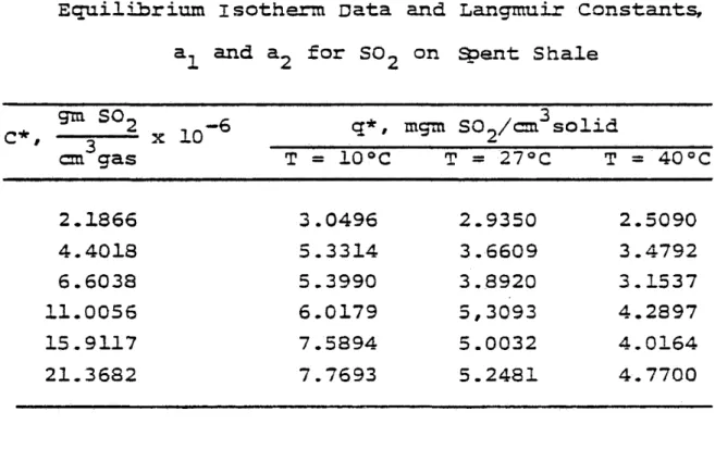
TABLE IX

Equilibrium isotherm Data and Langmuir Constants, a, and a_ for S09 on Spent. Shale

gm SO- ^ C*, 3 2 x 10- 6

q*»

T1998 ₄₅ © *o o r B & s « e u a c E 3 Li XI 3 3* ca CM ^5* _OJ CM © w 3 D» •*4 Cb CM -O •XD cu .olx ancs c“» / :os ^ '♦& C #. { jih S 0 t / ci ii j pi X 10 4

L e a s t S q u a r e Fi t fo r F r e u n d l i c h M o d e l at T = 2 7 ° C F i g u r e (/ /* ) T1998 47

L e a s t S q u a r e Pi t fo r F r e u n d l i c h M o d e l at T = 4 0 ° C

T1998

TABLE X

Equilibrium Isotherm Data and Freundlich Constants for S02 on Spent Shale

gm S O , -* , — 3— 2- x 1 0 ~ 6 cm gas <2*, 3 mgm S0 2/cm s o l i d Hi It H O 0 _{O T = 27°C T = 40 °C} 2.1866 3.0496 2.9350 2.5090 4 • 4018 5.3314 3.6609 3.4792 6.6038 5.3990 3.8920 3.1537 11.0056 6.0179 5.3093 4.2897 15.9117 7.5894 5.0032 4.0164 21.8682 7.7693 5.2481 4.7700 Temperature, °C K 1 /n 1 0 496.3011 X 1 0 ~ 3 381.44 x 1 0 ~ 3 27 105.2423 X 1 0 ~ 3 270.20 x i o ~ 3 40 72.6734 X 1 0 ~ 3 255.15 x 1 0 - 3

E q u i l i b r i u m Da ta Fi t to F r e u n d l i c h M o d e l o o o o go csi

L e a s t S q u a r e Pi t fo r D u b i n i n M o d e l at 1 0 ° C T1998 51 tM CO T CU CD ( TO T M fiox

L e a s t S q u a r e Pi t fo r D u b i n i n M o d e l at 2 7 ° C CO CD o AA 6o|

[

l

o

g

i

n

(

p

n

/

p

)l