Analysis Strategy for Fracture
Assessment of Defects in
Ductile Materials
Research
Authors:2009:27
Peter Dillström Magnus Andersson Iradj Sattari-Far Weilin ZangTitle: Analysis Strategy for Fracture Assessment of Defects in Ductile Materials. Report number: 2009:27.
Authors: : Peter Dillström, Magnus Andersson, Iradj Sattari-Far and Weilin Zang. Inspecta Technology AB, Stockholm, Sweden .
Date: June 2009.
This report concerns a study which has been conducted for the Swedish Radiation Safety Authority, SSM. The conclusions and viewpoints pre-sented in the report are those of the author/authors and do not neces-sarily coincide with those of the SSM.
Background
SSM has supported research for investigating the role of secondary stresses when fracture assessments are performed for cracked structures made of ductile materials. There are evidences that indicate that some secondary stresses, such as weld residual stresses, are not as important as primary stresses for estimating the safety margin against rupture (measured by the J-integral) for the type of ductile materials which can be found in nuclear power plants.
The project was initiated by SKI.
Objectives of the project
The objective of the project has been to perform numerical analyses of girth welds in pipes of different sizes for estimating the weld residual stresses and investigate how the weld residual stresses behave when cracks are introduced. Based on the results, an analysis strategy has been proposed on how the safety factor against these kinds of secondary stresses can be defined for evaluating pipe rupture in ductile materials.
Results
- For the studied cases with stainless steel welds or Alloy 182 welds in stainless steel piping, the relative contribution from the weld residual stresses to CTOD or J decreases rapidly for high values of the limit load parameter Lr. For very high values of Lr the analyses indicate that the contribution from the weld residual stresses to fracture becomes negligible.
- The precise limit of Lr at which the relative contribution from the weld residual stresses is small is likely to depend on the particular material properties, crack geometry and the weld residual stress distribution.
- Based on the analysis result, a new deterministic safety evaluation system is proposed. In the procedure, new safety factors against the fracture toughness are defined where it is distinguished between primary and secondary stresses. Based on the predicted value of Lr at fracture, the safety factor against the local through-thickness secondary stress is lowered. This is assumed also to be valid for thermally induced through-thickness stress gradients. However, no change in safety factor is proposed for global secon-dary stresses such as thermal expansion stresses.
Effects on SSM
The results of this project will be of use to SSM in safety assessments when cracks are detected in nuclear power plant components. However, SSM wants to further validate the analysis results in this project and the proposed revision of the deterministic safety evaluation system by performing experiments. Such experiments are planned in an ongoing research project.
Project information
Project Leader at SSM: Kostas Xanthopoulos Project number: 14.42-011210/22094
Project Organisation: Inspecta Technology AB has been managed the pro-ject with Peter Dillström as propro-ject leader. Magnus Andersson, Iradj Sattari-Far and Weilin Zang have assisted in the development of the project.
SUMMARY
The main purpose of this work is to investigate the significance of the residual stresses for defects (cracks) in ductile materials with nuclear applications, when the applied primary (mechanical) loads are high. The treatment of weld-induced stresses as expressed in the SACC/ProSACC handbook and other fracture assessment procedures such as the ASME XI code and the R6-method is believed to be conservative for ductile materials. This is because of the general approach not to account for the improved fracture resistance caused by ductile tearing. Furthermore, there is experimental evidence that the contribution of residual stresses to fracture diminishes as the degree of yielding increases to a high level. However, neglecting weld-induced stresses in general, though, is doubtful for loads that are mostly secondary (e.g. thermal shocks) and for materials which are not ductile enough to be limit load controlled.
Both thin-walled and thick-walled pipes containing surface cracks are studied here. This is done by calculating the relative contribution from the weld residual stresses to CTOD and the J-integral. Both circumferential and axial cracks are analysed. Three different crack geometries are studied here by using the finite element method (FEM).
(i) 2D axisymmetric modelling of a V-joint weld in a thin-walled pipe. (ii) 2D axisymmetric modelling of a V-joint weld in a thick-walled pipe. (iii) 3D modelling of a X-joint weld in a thick-walled pipe. t.
Each crack configuration is analysed for two load cases; (1) Only primary (mechanical) loading is applied to the model, (2) Both secondary stresses and primary loading are applied to the model.
Also presented in this report are some published experimental investigations conducted on cracked components of ductile materials subjected to both primary and secondary stresses.
Based on the outcome of this study, an analysis strategy for fracture assessment of defects in ductile materials of nuclear components is proposed. A new deterministic safety evaluation system is defined, that more realistically handles the contribution to J or CTOD from secondary stresses. In the new procedure we define new safety factors against fracture described by K and differentiate between I Primary
K
SF (relating to primary stresses) and Secondary
K
SF (relating to secondary stresses). The procedure is consistent with the presented analyses and experimental data.
TABLE OF CONTENT
Page
1 INTRODUCTION ...5
2 ANALYSIS OF INTERNAL CIRCUMFERENTIAL SURFACE CRACKS IN THIN-WALLED PIPES ...7
2.1 Simulation of the welding process and crack growth ...7
2.1.1 Finite element modelling...7
2.1.2 Thermal analysis ...8
2.1.3 Structural analysis... 10
2.1.4 Simulation of crack growth ...11
2.2 A welded pipe subjected to a primary load ...12
2.2.1 Contribution from residual stresses to J and CTOD using an axial loading... 12
2.2.2 Relaxation of residual stresses due to unloading ...17
2.2.3 Effect of tangent modulus ...18
2.2.4 Effect of using linear isotropic hardening ...23
2.3 A welded pipe subjected to a thermal load...24
2.4 Discussion on the results for thin-walled pipes ...29
3 ANALYSIS OF INTERNAL CIRCUMFERENTIAL SURFACE CRACKS IN THICK-WALLED PIPES ... 31
3.1 Geometry... 31
3.2 Material data... 32
3.3 Element mesh ... 33
3.4 Loading and boundary conditions... 35
3.4.1 Simulation of the weld process ... 35
3.4.2 Simulation of crack growth ...35
3.4.3 Primary load ... 36
3.5 Results ...36
4 ANALYSIS OF INTERNAL AXIAL SURFACE CRACKS IN THICK-WALLED PIPES ...42
4.1 Geometry... 42
4.2 Material data... 42
4.3 Element mesh ... 42
4.4 Loading and boundary conditions... 44
4.4.1 Simulation of the weld process ... 44
4.4.2 Simulation of crack growth ...44
4.4.3 Primary load ... 44
4.5 Results ...44
5 EXPERIMENTAL RESULTS ... 51
5.1 Wilkowski and Rudland, Battelle, USA... 51
5.2 Dong et. al., Battelle, USA ...52
5.3 Mohr et. al., Edison Welding Institute, USA...52
5.4 Sharples et. al., AEA Technology, UK ... 54
5.5 Sharples and Gardner, AEA Technology, UK...56
5.6 The IPIRG project, Battelle, USA ... 57
5.7 Lei et. al., Imperial College, UK... 59
5.8 Discussion ... 60
6 A STRATEGY FOR FRACTURE ASSESSMENT OF DEFECTS IN DUCTILE MATERIALS ... 61
6.1 Motivation for a new strategy for fracture assessment of defects in ductile materials ...61
6.2 Case study 1, a thin-walled pipe containing a circumferential surface crack ... 62
6.3 Case study 2, a thick-walled pipe containing a circumferential surface crack ... 65
6.4 Case study 3, a thick-walled pipe containing an axial surface crack ...67
6.5 Case study 4, components with through-wall cracks ... 69 6.6 Recommendations for a new procedure for fracture assessment of defects in ductile materials .71
6.6.2 Application of the new deterministic safety evaluation system... 76
7
IMPLEMENTATION OF THE NEW PROCEDURE IN THE FRACTURE
ASSESSMENT SOFTWARE PROSACC ...80
7.1 Estimation of safety factors in the new deterministic safety evaluation system... 80
7.1.1 Safety factors for a normal/upset load event, SFK = 3.162... 81
7.1.2 Safety factors for an emergency/faulted load event, SFK = 1.414 ...81
7.2 Choice of options within the ProSACC software ...82
8 CONCLUSIONS AND RECOMMENDATIONS ...83
9 ACKNOWLEDGEMENT...85
10 REFERENCES ... 86
APPENDIX A. THE J-INTEGRAL AND CTOD AS FRACTURE PARAMETERS... 89
APPENDIX B. CALCULATION OF CTOD ... 93
APPENDIX C. LIMIT LOAD OF 2D MODEL ... 95
1
INTRODUCTION
Structures may fail because of crack growth both in welds and in the heat affected zone (HAZ). The welding process itself induces residual stresses in the weld and HAZ, which contribute to crack growth. The mechanism of growth can be sub critical i.e. IGSCC or fatigue, or critical growth initiation. Two examples of crack growth in welds are studied by Kanninen et al. [1981] and by Hou et al [1996]. So far, it is not self evident which characterising fracture parameter to use when the crack is subjected to weld-induced stresses. The results presented in the scientific literature indicate difficulties in using the J-integral as fracture parameter when residual stresses are present. Some researchers have proposed to use CTOD (Crack Tip Opening Displacement) as a suitable fracture parameters when secondary stresses are also present in the component, see for instance Kanninen et al. [1981] and Hou et al. [1996].
In this report both the J-integral and CTOD (obtained by the 90°-interception construction) are evaluated using finite element analysis, and their validity and usefulness as suitable fracture parameters are discussed.
The main purpose of this work is to investigate the significance of the secondary stresses for defects (cracks) in ductile materials within nuclear applications. The treatment of weld-induced stresses as expressed in the SACC handbook by Andersson et al [1996] is believed to be too conservative for ductile materials. This is because of the general approach does not to account for the improved fracture resistance caused by ductile tearing and furthermore there is experimental evidence that the contribution of residual stresses to fracture diminishes as the degree of yielding increases to a high level. Green et al [1993, 1994] and Sharples et al [1993, 1995, 1996] showed in a series of experiments that at low load levels, i.e. small Lr, the influence of the residual stresses was large, but near plastic instability (Lr = 1) weld-induced stresses were of little importance. Available procedures for flaw assessments, such as the ASME XI code and the R6 procedure [Milne et al, 1988] treat this issue differently. For instance, the ASME XI code does not consider weld-induced residual stresses in some materials e.g. stainless steel welds. Neglecting weld-induced stresses in general, though, is doubtful for loads that are mostly secondary (e.g. thermal shocks) and for materials which are not ductile enough to be limit load controlled. Several references regarding simulation of the welding process can be found in the literature, see for instance Brickstad and Josefson [1996] and Hou et al. [1996].
The purpose of this study is to investigate the significance of the secondary stresses (mainly weld residual stresses has been studied) for cracks in pipes of ductile materials. Both thin-walled and thick-walled pipes are studied. This is done by calculating the relative contribution from the weld residual stresses to CTOD and the J-integral. Both circumferential and axial cracks are analysed. However, the conclusions from this study are also valid for others components made of ductile materials.
Three different crack geometries are studied here, by using the finite element method (FEM).
- The first analysis is a 2D axisymmetric modelling of a V-joint weld in a thin-walled pipe. The crack introduced in this analysis is a complete circumferential internal surface crack in the centre of the weld. The results of this analysis are given in Chapter 2 of this report.
- The second analysis is similar to the first analysis, but for a thick-walled pipe. The results of this analysis are given in Chapter 3 of this report.
- The third analysis is a 3D modelling of an X-joint weld in a thick-walled pipe. The crack geometry in this analysis is a semicircular axial internal surface crack in the centre of the weld. The results of this analysis are given in Chapter 4 of this report.
Each crack configuration is analysed for two load cases:
- Only primary (mechanical) loading is applied to the model.
- Both secondary stresses and primary loading are applied to the model.
The steps in the analyses of the cases subjected to both primary and secondary stresses are given below:
- The welding process is simulated to introduce weld residual stresses (secondary stresses) in the model of the pipe.
- The crack is introduced within the model.
- A primary load is applied. For this “combined” loading case, the fracture mechanics parameters J and CTOD are calculated.
The relative contribution from the secondary stresses (mainly weld residual stresses in this study) is calculated in this report according to the following definitions:
CTOD CTOD
CTOD
CTOD
combined primary contribution from residual stresses
primary
combined primary contribution from residual stresses
primary J J J J (1-1) where
- CTODcombined,Jcombined CTOD and J calculated from load cases with both weld residual stresses and primary loading.
- CTODprimary,Jprimary CTOD and J calculated from load cases with primary loading only. Details of these analyses are previously reported by Delfin et al. [1997] and Andersson and Dillström [2004].
This report covers the main parts of these two reports. Also presented in this report are some published experimental investigations conducted on cracked components of ductile materials subjected to both primary and secondary stresses. Based on the outcome of these results, an analysis strategy for fracture assessment of defects in ductile materials of nuclear components is proposed in Chapter 6 of this report. Implementation of this analysis strategy into the fracture assessment software ProSACC is given in Chapter 7 of this report.
2
ANALYSIS OF INTERNAL CIRCUMFERENTIAL SURFACE CRACKS IN
THIN-WALLED PIPES
The finite element analysis of thin-walled pipes containing circumferential cracks subjected to welding residual stresses and mechanical loads is briefly presented in this section. More details of this analysis are given in Delfin et al. [1997].
2.1
Simulation of the welding process and crack growth
The modelled pipe has an inner radius, ri = 38 mm and a wall-thickness, t = 11 mm. The geometry is depicted in Fig. 2.1. The weld is oriented circumferentially. The choice of geometry is guided by the type of stress field obtained for thin walled pipes. The axial stresses are essentially through-thickness bending, whereas in a thick-walled pipe they are more complex and also less severe. A non-linear uncoupled thermoplastic based model was used. The thermal analysis and the stress analysis are described in the two following subsections. The general procedure of simulation follows that of Brickstad and Josefson [1996].
The geometry of the weld modelling is simplified in the following ways:
- Only the last weld pass is modelled. This is motivated by the fact that for a thin-walled pipe, as in this case, the last weld pass in a series of passes will cause a uniform heating of the entire thickness of the pipe.
- Only half of the pipe section is modelled since the crack plane coincides with the symmetry plane.
- It has been observed that the residual stresses in a circumferentially welded thin-walled pipe are approximately rotationally symmetric. This justifies the use of an axisymmetric model.
- The weld geometry is somewhat simplified, since a rectangular groove has been used.
2.1.1 Finite element modelling
The same mesh has been used in both the thermal and the stress analysis. The elements used are eight-noded biquadratic axisymmetric elements with full integration, which have proved to give the best convergent behaviour. The crack plane is also the symmetry plane which allows for the modelling of only half the pipe section, see Fig. 2.1. Anticipating that a crack is to be introduced, the mesh is focused on a point where the crack-tip will be located. The smallest elements used are of sizes 0.001 mm. This was necessary in order to evaluate the CTOD at low load levels. The FEM code ABAQUS [1995] uses a Newton iteration method improved by a line search algorithm, which is effective when the initial iterations are relatively far from the solution.
Fig. 2.1. a) The geometry of a cross section of the pipe wall in the z-direction. Only half the pipe is shown due to symmetry. b) Detail of the mesh used in the finite element analysis.
2.1.2 Thermal analysis
The thermal problem was treated as follows: A heat flux [W/m3] was activated in the weld material that constitutes the last weld pass. The use of only the last weld pass simplifies the calculations substantially in the respect that birth of elements need not be considered. An unrealistic consequence of the assumption of axial symmetry is that the heat flux is applied instantaneously around the circumference of the pipe. This can to some extent be compensated for by assuming that the heat flux is applied during a finite period in time with an assumed triangular time variation corresponding to the approach and passing of the weld torch. The heat flux h can be expressed as
line p v h Q V (2-1)
where Qline is the net line energy [J/m] used during the welding and v is the travel speed of the weld electrode, Vp is the weld pass volume. However the weld pass volume Vp can not be defined in a 2-D model and must be chosen in such a way that some empirical observations are satisfied. The molten zone size and the distance from the weld-base material interface to HAZ must be realistic, see Brickstad and Josefson [1996]. Once its value has been set the duration t of the heat flux period can
be determined from p p V t A v (2-2)
where Ap is the area of the cross section of the weld pass. However it should be pointed out that the objective here is to achieve a relatively high residual stress levels and properly infer the residual stresses through plastic strains, rather than simulating a particular stress field.
The boundary conditions allow for both convection and radiation. The axisymmetric conditions assumed imply that the heat losses in the axial direction are neglected. Radiation losses are dominant for higher temperatures near the weld. Convection losses are important for lower temperatures some distance away from the weld. A combined boundary condition, which takes both radiation and convection into account, is used in this work, Argyris et al [1983]. The resulting heat transfer coefficient h is 2 o 2 o 0.0668 (W/m ), for 0 500 C 0.231 82.1 (W/m ), for 500 C h h T T T T (2-3)
The other necessary thermal data for both the weld and base material are given in Table 2.1. Table 2 1. Thermal properties used in the FEM analysis.
2.1.3 Structural analysis
In the structural analysis the temperatures taken from the thermal analysis are used to calculate the stresses. Only small strain theory is considered. In Brickstad and Josefson [1996], it was observed that the difference in the weld-induced stresses between small strain theory and large strain theory is small. The von Mises yield criterion and associated flow rule are used together with kinematic hardening and a bilinear representation of the stress strain curve. Kinematic hardening rather than isotropic hardening is chosen because it is believed to better model reverse plasticity and the Bauschinger effect that is expected to occur during welding. It is also believed that an insufficient number of stress cycles occur during the single-pass welding for symmetrization of the hysteresis loop to occur, a situation which would have been better represented by isotropic hardening. The use of only the last weld pass simplifies the calculations in the same way as in the thermal analysis in the respect that birth of elements need not be considered. The material in both the weld and the base has the same mechanical properties. This choice serves the purpose of limiting the number of parameters affecting the fracture problem. The mechanical properties used in the analysis are presented in Table 2.2.
Table 2.2. Mechanical properties used in the FEM analysis.
The resulting axial stress across the symmetry line at T = 22.5 °C is shown in Fig. 2.2. For this relatively thin-walled pipe the stress distribution is mainly that of bending. The small bump at the weld pass boundary is believed to be a consequence of the numerical modelling. The crack will be introduced with its crack-tip located at 3.26 mm from the inside surface, which is not close to the bump. Thus, the bump will not be of any significance for the fracture analysis.
Fig. 2.2. The axial residual stress along the symmetry line i.e. in the weld centre line.
2.1.4 Simulation of crack growth
After the welding process is conducted and the pipe has cooled down to room temperature a crack is introduced at the weld centre line by means of gradual node relaxation starting from the inside of the pipe. The final crack depth is 3.26 mm. The axisymmetry of the problem allows only for a completely circumferential crack to be modelled. The crack is restricted to grow in the radial direction. A physical growth mechanism can be stress corrosion or fatigue. The chosen method of sequentially releasing the nodes along the chosen growth direction gives a path dependent J-integral. This is simply because growth does not represent proportional loading. When the crack reached its final length, loads will be applied and as the loads are increased the J-integral becomes, from a practical view, path independent.
2.2
A welded pipe subjected to a primary load
2.2.1 Contribution from residual stresses to J and CTOD using an axial loading
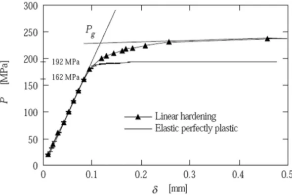
An axial tensile load was applied to the pipe both with and without residual stress present. As the axial load, which is a primary load, was increased in very small steps the J-integral and the CTOD were calculated. The limit load parameter Lr is defined as P/Pg where P is the applied load and Pg is the limit load. For P = Pg the ligament is deformed plastically. In Fig. 2.3 the load-displacement curve
P - is presented and Pg is determined by the intersection of the two straight lines shown. The displacement, , is evaluated at the loading point. The value of the limit load is found to be Pg = 228 MPa. In this way it is possible to define a limit load from the finite element solution which in a sense is more physically motivated than for example handbook solutions, where the material is assumed to behave elastic perfectly-plastic. This Lr-solution is used throughout this paper. The solution obtained from the handbook Andersson et al. [1996], which assumes that the material behave elastic perfectly-plastically, gives Pg = 162 MPa. The difference between these two definitions of Pg is quite significant. This can be explained by the effect of hardening and by the way the von Mises criterion is fulfilled. The introduction of a crack makes it possible for the stress components to redistribute in such a way that the axial stress becomes greater than the yield stress in the ligament, which is not allowed for in the handbook solution. To demonstrate the effect of this stress redistribution, the P - curve for the considered material with vanishing hardening, is also shown in Fig. 2.3. The elastic perfectly-plastic limit load is then found to be 192 MPa.
Fig. 2.3. Load versus the displacement at the end of the pipe.
The definition of Pg is somewhat arbitrary. Other limit load solutions may be used and the results may then be calibrated accordingly by multiplying the Lr scales in Fig. 2.4 to Fig. 2.9 by an appropriate factor.
The following three figures show the comparisons of J (Fig. 2.4), CTOD (Fig. 2.5), the relative contribution from residual stresses to J and CTOD (Fig. 2.6), during axial loading. The relative contribution from the weld residual stresses is calculated according to Equation (1-1).
Fig. 2.4a. The J-integral as a function of Lr. The J-values are evaluated at the tenth contour i.e. a ring with a radius of nine elements from the crack tip.
A short description on J and CTOD as fracture parameters for welded structures is given in Appendix A. Also, a method to evaluate CTOD from finite element analyses is given in Appendix B.
Fig. 2.5a. The CTOD as a function of Lr.
The principal behaviour of the J-integral is as expected for primary loads. The curve in Fig. 2.4 is essentially composed of an elastic part and a plastic part with a steep slope; see Bergman [1991] for a review on differences between primary and secondary loads. The results of Kumar et. al. [1991] are quite similar, though they used a thermal load as secondary load.
An evaluation of the case using a combination of an axial load and residual stresses according to the R6-procedure is also included in Fig. 2.4. The R6-procedure gives a slightly non-conservative estimation between Lr = 0.95 and Lr = 1.2. However it should be remembered that Lr is not defined by a limit load equal to 162 MPa as would normally be the case in a standard handbook solution, such as Andersson et al. [1996], instead a definition of the limit load equal to 228 MPa based on fully plastic behaviour, as shown in Fig. 2.3, is used.
It is interesting to quantify the relative contribution from the residual stresses during axial loading for both the J-integral and the CTOD. In Fig. 2.6a below, the relative differences between J with both residual and axial stresses present, Jcombined, and J with only axial stresses present, Jaxial, are shown. The same type of quantity formed with J replaced by CTOD, is plotted in Fig. 2.6b below. The CTOD could not be evaluated for Lr less than about 0.7 for the case with only axial loading despite the fine mesh. The irregular behaviour for the case with both residual stresses and axial stresses present for Lr less than about 0.8 can be explained by path dependency of J at low axial load levels, which is a result of the stress history due to crack growth.
The close coincidence of the J-curves and the CTOD curves in Fig. 2.6 suggests that the relation in equation (2-4) holds. This suggests also that J can be a possible fracture parameter if the integration contours are not far from the crack-tip. However only an experimental investigation can give a definite answer to the question of whether J or CTOD can be useful fracture parameters during this type of loading situation with residual stress- and strain-fields present. The contribution to the fracture parameters from the residual stresses is negligible for large Lr as shown in Fig. 2.6b. The contribution from the residual stresses decreases rapidly between Lr = 0.8 and Lr = 1.3. For Lr = 1.3 the contribution of the residual stresses is 20% of the axial load contribution. For Lr = 1.6 the contribution of the residual stresses is about 7%. An important observation is that this makes it essential to have a reliable value for Lr when plastic failure occurs i.e. when Lr = Lr
max
. In the present investigation the value of Lr at plastic collapse can not be defined. This is due to the linear hardening material model adopted (with its bilinear representation). Reasonably close to Lr = 1.0 the results should be valid also for other type of hardening behaviour. However, the results should be viewed with caution if a quantitative conclusion is desired. This is because the results are qualitative in the sense that a particular geometry and material model are chosen in this work.
Fig. 2.6a. The relative difference of J and CTOD with and without residual stresses.
Fig. 2.6b. Close up for a better resolution at high Lr-values.
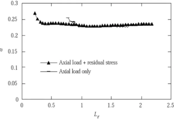
The parameter d is shown in Fig. 2.7 below, for the load cases with and without residual stresses. The non-dimensional parameter d is defined through the relation, c.f. Shih et al [1981],
CTODd J SSY (2-4)
Fig. 2.7. The values of the non-dimensional parameter d as a function of Lr. The parameter d is defined according to Eq. (2-4).
The values of d in Fig. 2.7 for both the case with the residual stresses present and the case with only axial stresses, are scattered very little from the value 0.23. This means that at least in this investigation the J-integral is well defined through Equation (2-4) with d = 0.23. However remember that for J evaluated with remote contours the J-integral seems definitely path dependent. Appendix A provides a discussion of this problem. The reason for the cut-off at Lr = 0.8, for the case of axial loading only, is that CTOD could not be evaluated even with the fine mesh used. The corresponding cut-off for the case of both axial loading and residual stresses is Lr = 0.25. In this case CTOD may be undefined because of the crack growth prior to the application of axial loading, see Appendix B.
2.2.2 Relaxation of residual stresses due to unloading
To investigate the effect of relaxation, unloading were performed for the uncracked geometry from different axial load levels, see Fig. 2.8. The stress distribution along the symmetry line may serve as an input in an engineering estimation e.g. a fracture assessment according to the R6-procedure. It is not relevant to unload the cracked pipe since the J-integral and the CTOD become meaningless in this type of unloading situations.
Fig. 2.8. The axial stresses at the symmetry line after unloading. The Lr-values represent the different load levels from which the unloading was performed.
The resulting levels of the residual stress distributions, after unloading, decreases with increasing Lr, and does not change for load levels larger than Lr = 0.8. For a circumferential surface crack, on the inside of the pipe, not deeper than 40% of the wall-thickness, there will clearly be only very small residual stresses after unloading from a high level of axial load. The stress peak of 80 MPa for the case
Lr = 0.8 is located about 70% of the wall thickness from the inside of the pipe, through the wall.
2.2.3 Effect of tangent modulus
The chosen bi-linear kinematical hardening material model limits the analyses in two ways. It can only approximately account for the more realistic non-linear hardening behaviour of materials. Secondly, a point of plastic collapse can not be defined, in our notation, this means that no max
r
L exists. This section addresses those limitations.
To get some understanding on how these limitations affect conclusions, a series of runs was performed on the same pipe geometry. The material models were the same except for a different tangent modulus, ET. The residual stresses, CTOD and J, the relative differences, (Jcombined - Jaxial)/Jaxial and (CTODcombined - CTODaxial)/CTODaxial were calculated and the results are shown in Fig. 2.9 to Fig. 2.12. In Fig. 2.9 it can be seen that for ET/E = 0.0001, which is nearly perfectly plastic material behaviour, the residual stresses attain the highest tensile stress level. The stress distribution changes shape somewhat but the stress level does not change very much with different amount of hardening. Note however that close to the inside of the pipe the stresses are fairly independent of the tangent modulus.
Fig. 2.9. Axial residual stresses at the weld centreline for ET/E = 0.0001, 0.005, 0.01, 0.014, 0.018. The limit load Pg definition, with graphical determination, used in section 2.1.1 is not appropriate here. In order to compare J and CTOD using the same scale, Lr is defined as Lr
R6 = P/Pg
R6
where Pg
R6 is the limit load used in the R6-method and in the handbook of Andersson et al. [1996].
For the same Lr-value, more plasticity is introduced with decreasing hardening. This is consistent with the behaviour of the J - Lr and the CTOD - Lr curves, Fig. 2.10 and Fig. 2.11, which rise steeper with decreasing hardening.
Fig. 2.10a. Jaxial (axial load only) as a function of Lr for different ET/E.
Fig. 2.11a. CTODaxial (axial load only) as a function of Lr for different ET/E.
The relative differences of J and CTOD, Fig. 2.12, vanish at a higher rate the lower the hardening is. For ET/E = 0.0001 there is no curve because Lr does not get higher than Lr = 1.25 because of widespread plasticity.
Fig. 2.12a. The quantity (Jcombined - Jaxial)/Jaxial as a function of Lr for different ET/E.
The lowering of hardening has thus the effect of reducing the contribution from the residual stress to J or CTOD. In a real material the same should occur as Lr approaches Lmaxr. This implies that not only does the contribution from residual stresses decrease with increasing Lr but also that an additionally decreasing effect due to decreasing hardening, should be taken into account for high Lr-values.
2.2.4 Effect of using linear isotropic hardening
Although a very exact model of the hardening behaviour during welding certainly would be very complex, including both expansion and translation of the yield surface in stress space, it is believed that kinematic hardening models the plastic behaviour better than isotropic hardening. To study the effect of the chosen hardening model, the J-integral and CTOD were also calculated assuming linear isotropic hardening with and without weld residual stresses during axial loading of the pipe. It is seen in Fig. 2.13 that the choice of hardening behaviour is important. When using isotropic hardening, the stresses are unloaded, close to the crack-tip, during part of the loading history. This is reflected in the negative J-values at Lr = 1.25. In fact for Lr = 1 it would be more favourable to include the residual stresses than not to include the residual stresses. The trend for CTOD is the same. The results are similar to those of Hou et. al. [1996], who also used a linear isotropic hardening model.
Fig. 2.13b. The CTOD as a function of Lr, with isotropic hardening.
2.3
A welded pipe subjected to a thermal load
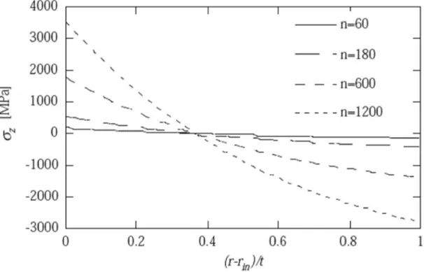
A thermal load was applied to the pipe with a circumferential surface crack both with and without the residual stresses present. The thermal load was imposed by specifying a radial temperature distribution in the pipe according to
( ( )) ( ) 22.5 exp( ) i i r r t T r n r r t (2-5)
which is presented together with the resulting axial stresses for the linear elastic case in Fig. 2.14. As the thermal load was increased in very small steps by increasing the value of the scaling parameter n in Equation (2-5), the J-integral and the CTOD were calculated. A limit load parameter can not be defined for the type of secondary thermal load used here since the pipe can not yield completely.
Fig. 2.14a. The temperature distribution through the thickness of the pipe (according to Equation (2-5)).
Fig. 2.14b. The corresponding axial stress distribution through the thickness of the pipe (for the linear elastic case).
The thermal load at which the innermost fibre begins to yield may serve as a point of reference. This occurs when 1.27 (1 ) Y E T (2-6)
where T = 20°C - T, i.e. the difference in temperature between room temperature and the temperature T at r = ri in Equation (2-5).
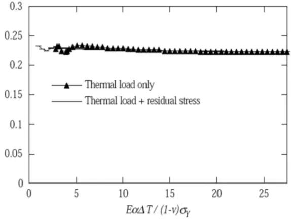
Fig. 2.15, Fig. 2.16 and Fig. 2.17 show the comparisons of J, CTOD and d respectively, for the different temperature distributions, as given in Fig. 2.14a, with and without the residual stress present. The behaviour of J and CTOD is similar. It is related through the non-dimensional parameter d according Equation (2-4). In Fig. 2.17, it is shown that the value of d is 0.23, which is the same as determined for the case of an axial loading.
Fig. 2.15b. The J-integral as a function of a non-dimensional load parameter (close up for low values of the load parameter).
The loading curves for J (see Fig. 2.15) and CTOD (see Fig. 2.16 below) are very different from the corresponding curves for the pipe subjected to an axial load. This is because the thermal load is secondary and cannot cause plastic collapse. There is always a portion of the pipe cross section that does not yield. An important consequence of this is that the contribution of the residual stresses is approximately constant in absolute terms during the increase of the thermal load. The smallest contribution of residual stresses is found for low load levels. It must be remembered, however, that for low load levels the values of J are less reliable because of the effect of crack growth prior to loading.
Fig. 2.1a. The CTOD as a function of a non-dimensional load parameter.
Fig. 2.2b. The CTOD as a function of a non-dimensional load parameter (close up for low values of the load parameter).
Fig. 2.17. The values of the non-dimensional parameter d as a function of Lr. The parameter d is defined according to Equation (2-4).
2.4
Discussion on the results for thin-walled pipes
The main result of the study by Delfin et. al. [1997] is shown in Fig. 2.6. The relative contribution as defined in Fig. 2.6 from the residual stresses to CTOD or J decreases rapidly between Lr = 0.8 and Lr = 1.3. For Lr = 1.25 the relative contribution from the residual stresses is 20% compared to the axial load. For very high Lr-values the contribution becomes negligible. Thus, for the particular pipe studied the contribution of the residual stresses is negligible only for very high values of Lr. However, because of the linear hardening material model adopted (with its bilinear representation), plastic collapse can not be defined. This means that one do not know for a particular value of Lr, exactly how far the load is from a fully plastic situation corresponding to true plastic collapse.
In the work by Kumar et al [1991] the contribution of a thermal load to the J-integral during a mechanical loading has been studied. They concluded that thermal loads can be neglected for high mechanical loads. A corresponding analysis made with a much more severe thermal loading than in the work by Kumar et al [1991], showed that the contribution to J from the thermal stresses can be significant also for Lr larger than 1. In this case, the value of Lr must be raised to more than 1.4 for the relative contribution from the thermal stresses to be small.
Green et al [1993, 1994] proposed that residual stresses need not to be included in fracture assessments of austenitic steels if Lr is larger than the ratio of the 1% proof stress to the 0.2% proof stress. In the present study this would correspond to an Lr -value of about 1.1. The investigation in Delfin et. al. [1997] indicates that this limit should be larger, approximately Lr = 1.3. If it can be
The opinion in Delfin et. al. [1997] is that great care must be taken in the treatment of the contribution of welding residual stresses or thermal stresses in fracture assessments. The results with proper simulation of the weld-induced stresses do support the idea of giving weld residual stresses a lower weight in a fracture evaluation if high primary loads are present. However, the limit of Lr at which the relative contribution from weld residual stresses (or thermal loads) to CTOD or J is small enough, is likely to depend on the particular material model, crack geometry and the shape and level of the residual (or thermal) stress distribution. More analyses needs to be done (and also a comparison with experimental data), which is presented in the following sections of this report.
3
ANALYSIS OF INTERNAL CIRCUMFERENTIAL SURFACE CRACKS IN
THICK-WALLED PIPES
The finite element analysis of thick-walled pipes containing circumferential surface cracks subjected to welding residual stresses and mechanical loads is briefly presented in this section. More details of this analysis are given in Anderson and Dillström [2004].
3.1
Geometry
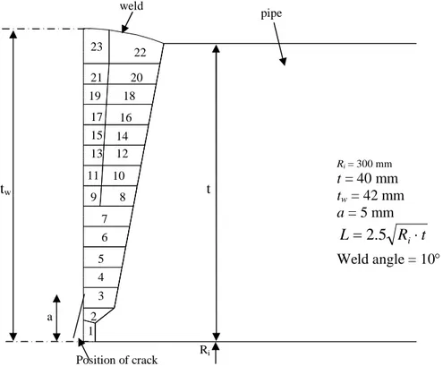
The analysed pipe is thick walled with an inner radius of 300 mm and a thickness of 40 mm. The geometry is taken from Brickstad and Josefson [1996]. The weld is oriented circumferentially and consists of 36 passes in 15 layers through the thickness. However since only half of the pipe is modelled due to symmetry only 23 passes are included in the model, see Fig. 3.1 and Fig. 3.2. Number 1, 2, 9, 11, 13, 15, 17, 19, 21 and 23 of these passes are half passes due to symmetry.
Pipe
Weld
Symmetry
Fig. 3.1. Geometry of the welded pipe.
In the analysis, a crack is later introduced in the centre of the weld at the inside of the pipe. As the model is in 2D, the crack is fully circumferential. The crack depth is a = 5 mm.
Fig. 3.2. Geometry of the weld, with the 23 weld passes that were included in the model.
3.2
Material data
The material in both the pipe and the weld are stainless steel. The data are taken from Brickstad and Josefson [1996] and summarised in Table 3.1 and Table 3.2.
Table 3.1. Material data for pipe and weld, thermal analysis. Temperature T [˚C] Specific heat p C [J/kg ˚C] Conductivity
[W/m ˚C] Density
[kg/m3] 20 442 15.0 7840 200 515 17.5 7840 400 563 20.0 7840 600 581 22.5 7840 800 609 25.5 7840 1390 675 66.2 7840 1 2 3 4 5 7 6 9 8 10 11 13 12 15 14 17 16 20 19 18 21 22 23 tw t Ri Position of crack pipe weld a Ri = 300 mm t = 40 mm tw = 42 mm a = 5 mmt
R
L
2
.
5
i
Weld angle = 10Table 3 2. Material data for pipe and weld, structural analysis. Temperature T [˚C] Young’s modulus E [MPa] Poisson’s ratio
[-] Thermal expansion coefficient
[10 / °C
6 ] Yield stress y
[MPa] Plastic tangent modulus TE
[MPa]/
TE
E
[-] 20 200000 0.278 17.0 230 28000 0.14 200 17.5 400 170000 0.298 18.5 132 23800 0.14 600 19.0 800 135000 0.327 19.5 77 1890 0.14 1000 95000 0.342 20.0 50 9.5 1·10-4 1100 50000 0.350 20.03.3
Element mesh
The ABAQUS [2003] elements used for all 2D analyses were the eight nodes bi-quadratic axi-symmetric elements DCAX8 (thermal analysis) and CAX8 (structural analysis), both with full integration.
Anticipating that a crack is introduced and that CTOD is calculated for a primary loading in the interval
0.8
L
r
2
, the element size near the crack tip must be very small. The smallest element length is 2.510-3 mm, see Fig. 3.3. An analysis with a coarser mesh has also been done where the smallest element length was 2010-3 mm. With this coarser mesh similar results were obtained for CTOD whenL
r1.0
.Fig. 3.3. Element mesh of the pipe, weld and crack tip (smallest element length 2.510-3 mm). Crack tip y x Symmetry: uy= 0 uy equal Stress path
3.4
Loading and boundary conditions
Below, the different loadings are presented. The analysis consists of three phases, the welding process, crack growth and finally applying the primary loading. The boundary condition at the start of the analysis is an applied symmetry condition at the centre of the weld (u y 0). Also the axial degrees of freedom (dof), uy, are constrained to be equal at the free end of the pipe, see Fig. 3.3.
3.4.1 Simulation of the weld process
The technique to compute the weld induced residual stresses is described in detail in Delfin et. al. [1998]. The welding process simulation was done with an uncoupled thermo-plastic analysis. First a transient thermal analysis is performed during which the time dependent temperature distribution is determined for the successive build up of the welding passes. The stress field due to the temperature field is then evaluated at each time step in a structural analysis.
The weld is modelled by introducing the 23 passes successively. During the thermal analysis radiation and convection boundary condition are applied. These vary with each weld pass. The resulting heat transfer coefficient (including both radiation and convection),
h, is taken form Delfin et. al. [1998] and given by Equation (3-1).
2 o 2 o 0.0668 W/ m C 20 C 500 C 0.231 82.1 W/ m C 500 C h h T T T T (3-1)In the subsequent structural analysis the stresses are calculated with an elastic-plastic material model. The von Mises yield criterion with associated flow rule and bi-linear kinematic hardening is used. In Delfin et. al. [1997], it was observed that differences between analyses with small strain theory and large strain theory are small. Therefore only small strain theory is used. The multi pass weld is modelled by activating the elements belong to the current pass at a proper time during the transient phase. The elements are introduced strain-free.
3.4.2 Simulation of crack growth
After the welding process and after the pipe and weld have cooled, a crack is introduced in the centre of the weld starting from the inside of the pipe. The final crack length is a = 5 mm. The crack is introduced by releasing the constrained degrees of freedoms in the centre of the weld. The 2D axi-symmetric model allows only a complete circumferential crack to be introduced. The crack growth is restricted to the radial (x) direction. The method of releasing nodes along the chosen growth direction gives a path dependent J-integral. This has to do with the fact that the growth does not represent a proportional loading. However, when the primary loading is introduced and then increased to higher
r
3.4.3 Primary load
After the crack is introduced a primary load is applied. The load consists of an axial tension force applied at the free end of the pipe. The primary load is increased gradually to the final value
L
r2.0
. For differentL
r-values the J-integral and CTOD is computed. The limit load for this 2D crack geometry is calculated in Appendix C.3.5
Results
In Fig. 3.4 the axial stress ( ) in the centre of the weld (the stress path in Fig. 3.3) is shown as a 22
function of a normalised coordinate, u, through the thickness. The axial stress is shown for different phases of the analysis, after welding and after crack growth (a0.125 ). As can be seen, a t
singularity occurs at the crack tip and for u 0.45 the axial stress is not affected by the crack growth. The limit load parameter, L , is defined as r axial/axial,limit where axial is the applied axial load and
axial,limit
is defined in appendix C.
Fig. 3.4. Axial stress, in the centre of the weld, through the thickness of the pipe. u = 0 is located at the inside and u = 1.0 at the outside of the pipe. The crack depth a = 5 mm.
Fig. 3.5 and Fig. 3.6 show the difference in axial stress for L r 0.99 and L r 1.98 for the cases if the weld residual stresses are present or not. As can be seen the stress distribution for the case with residual weld stresses approaches the stress distribution for the case without weld residual stresses for
r
L -values greater than 1.0. Fig. 3.7 and Fig. 3.8 show the stress distribution in the weld and pipe after the weld simulation and after crack growth.
Fig. 3.5. Normalised axial stress distribution through the thickness (from the inside to the outside of the pipe) at the centre of the weld with and without weld residual stresses. The primary load level is Lr = 0.99.
Fig. 3.6. Normalised axial stress distribution through the thickness (from the inside to the outside of the pipe) at the centre of the weld with and without weld residual stresses. The primary load level is Lr = 1.98.
Fig. 3.7. Axial stress distribution [Pa] after welding.
Fig. 3.8. Axial stress distribution [Pa] after crack growth.
Fig. 3.9 and Fig. 3.10 show the path independence of the J-integral for higher L -values for the r
Fig. 3.9. The J-integral as a function of contour number for the load case with a primary loading only. The distance between the contours is approximately 0.0025 mm.
Fig. 3.10. The J-integral as a function of contour number for the load case with both primary and secondary loading. The distance between the contours is approximately 0.0025 mm.
In Fig. 3.11 and Fig. 3.12 the J-integral (for contour 8) and the CTOD-value are shown as a function of L . As can be seen, the difference decreases for higher r L values. r
Fig. 3.11. The J-integral as a function of L for both load cases (with and without secondary loading). r
Fig. 3.12. CTOD as a function of L for both load cases (with and without secondary loading). r
In Fig. 3.13 and Fig. 3.14 (a comparison using two different contours when calculating J), this decreasing difference for higher L -values is shown as expressed in Equation (1-1). r
Fig. 3.13. The relative contribution of the weld residual stresses to J and CTOD according to Equation (1-1) for increasing L . Contour No. 8 is used. r
Fig. 3.14. The relative contribution of the weld residual stresses to J and CTOD according to Equation (1.1) for increasing L . Contour No. 20 is used. r
The contribution to the fracture parameters from the residual stresses is negligible for large Lr as shown in Fig. 3.13-3.14. The contribution from the residual stresses decreases rapidly with increasing
Lr. For Lr = 1.3 the contribution of the residual stresses is 10% of the axial load contribution. For Lr = 1.6 the contribution of the residual stresses is about 2%.
4
ANALYSIS OF INTERNAL AXIAL SURFACE CRACKS IN
THICK-WALLED PIPES
The finite element analysis of thick-walled pipes containing axial surface cracks subjected to welding residual stresses and mechanical loads is briefly presented in this section. More details of this analysis are given in Anderson and Dillström [2004].
4.1
Geometry
The analysed pipe is thick walled with an inner radius of 348.5 mm and a thickness of 84 mm, see Fig. 4.1. The geometry is taken from Delfin et. al. [1998] (type VI pipe). The weld is an X-joint, which is oriented circumferentially and consists of 21 passes. In the analysis an axial circular crack is also introduced in the centre of the weld at the inside of the pipe. Different crack depths was used (between
0.06 t a0.14 ). t
4.2
Material data
To simplify the analysis, the same material was used for both the pipe and the weld (Inconel 182). The data are taken from Delfin et. al. [1998] and summarised in Table 4.1.
Table 4.1. Material data for pipe and weld, Inconel 182. Temperature T [˚C] Young’s modulus E [MPa] Poisson’s ratio
[-] Thermal expansion coeff.
[10 / °C
6 ] Yield stress y
[MPa] Plastic tangent modulus TE
[MPa]/
TE
E
[-] 20 207000 0.324 13.0 380 2898 0.14 200 14.0 400 185000 0.301 15.3 302 25900 0.14 600 16.2 800 150000 0.320 17.0 185 2100 0.14 1000 125000 0.339 17.3 50 12.5 1·10-4 1200 50000 0.350 17.34.3
Element mesh
The ABAQUS elements [2003] used for all 3D analyses were the 20 nodes quadratic brick elements C3D20. For the 3D analysis it is not practical to use as small elements that were required for calculating CTOD for primary loading in the interval 0.8Lr2.0. The smallest element length in these analyses is approximately 0.5-0.8 mm. Fig. 4.1 shows the element mesh.
Fig. 4.1. Element mesh of the 3D model, with an axial crack. weld pipe Symmetry (ux=0) Symmetry (uy=0) a z x y Symmetry (uz=0) Crack tip Stress path uz equal Ri = 348.5 mm t = 84 mm
t
R
L
i
Weld angle = 15˚ 0.06·t ≤ a≤ 0.14·t4.4
Loading and boundary conditions
Below the different loadings are presented. As for the 2D case this analysis also consists of three phases, the welding process, crack growth and finally an applied primary loading. The boundary condition at the start of the analysis is an applied symmetry condition at the centre of the weld (u ) z 0 and at the parts where the pipe is cut, u and y 0 u respectively. Also the axial degrees of x 0 freedom, u , are constrained to be equal at the free end of the pipe, see Fig. 4.1. z
4.4.1 Simulation of the weld process
The technique to compute the weld induced residual stresses differs from the method used in the 2D analysis. This is due to the fact that the elastic-plastic analysis with element birth and death technique used in the 2D case is too time-consuming in the 3D case. Instead a simplified two step simulation to obtain the correct weld residual stresses is done. First the weld is given a temperature gradient through the thickness. This temperature gradient does not vary circumferentially. This applied temperature gradient leads to plastic deformation. In the next step the pipe is cooled down by setting the temperature uniformly to room temperature. The weld residual hoop stresses are then compared to the corresponding residual stresses obtained in a 2D analysis in Delfin et. al. [1998]. The same technique is used for weld simulation as the one for the 2D case in section 3 of this report. The von Mises yield criterion with associated flow rule and bi-linear kinematic hardening is used for the analysis.
4.4.2 Simulation of crack growth
After the welding process and after the pipe and weld have cooled, a circular axial crack is introduced in the centre of the weld starting from the inside of the pipe. The final crack depth is varied for different analyses in the interval of 0.06 t a0.14 , see Fig. 4.1. The crack growth is restricted to t
grow in the radial (x) direction only. As in the 2D case, the method of releasing nodes along the chosen growth direction gives a path dependent J-integral. This has to do with the fact that the growth does not represent a proportional loading. However, when the primary loading is introduced and increased to higher Lr-values, the J-integral becomes path independent from a practical standpoint.
4.4.3 Primary load
After the crack is introduced a primary load is applied. The load consists of internal pressure. However, the pressure is only applied in the radial direction (no axial component). The primary load is increased gradually to the final value L r 2.0. For different Lr-values the J-integral is computed. The limit load for this 3D crack geometry is calculated in Appendix D.
4.5
Results
In Fig. 4.2 the hoop stress ( ) in the centre of the weld (the stress path in Fig. 4.2) is shown as a 22
function of a coordinate through the thickness. The hoop stress is shown for different phases of the analysis, after welding and after crack growth (a0.08 ). All results are taken from a crack growth t
of a0.08 (unless otherwise stated). Similar results are obtained with different crack lengths (up to t
0.14
a ). The limit load parameter, t L , is defined as r p p/ limit where p is the applied load and plimit
Fig. 4.2. Hoop stress in the centre of the weld through the thickness. u = 0 is located at the inside of the pipe. The crack length a = 0.08t.
Fig. 4.2 also shows the corresponding residual weld hoop stress from Delfin et. al. [1998]. When comparing the residual stress profiles, it is evident that the approximation (using a temperature gradient) in this 3D analysis gives similar results as in the complete 2D analysis given in Delfin et. al. [1998]. The present 3D analysis is more conservative, i.e. gives larger residual stresses, for small cracks.
Fig. 4.3 and Fig. 4.4 show the difference in hoop stress for L = 0.93 and r L =1.98. In both figures a r
comparison is made for the cases when the weld residual stresses are present or not. As can be seen the stress distribution for the case with residual weld stresses approaches the stress distribution for the case without weld residual stresses for L -values greater than 1.0. r
Fig. 4.3. Normalised hoop stress distribution through the thickness (from the inside to the outside of the pipe) at the centre of the weld with and without weld residual stresses. The primary load level is L = 0.93. r
Fig. 4.4. Normalised hoop stress distribution through the thickness (from the inside to the outside of the pipe) at the centre of the weld with and without weld residual stresses. The primary load level is L = 1.98. r
Fig. 4.5 and Fig. 4.6 show the stress distribution in the weld and pipe after the weld simulation and after crack growth.
Fig. 4.5. Stresses in the circumferential direction [Pa] after welding.
Fig. 4.7 and Fig. 4.8 show the path independence of the J-integral for different contour paths. The distance between each contour number is 1.93 mm.
Fig. 4.7. J-integrals in different contour paths for the case without weld residual stress. Each curve
corresponds to a specific L . r
Fig. 4.8. J-integrals in different contour paths for the case with weld residual stress. Each curve
corresponds to a specific L . r
Increasing Lr
The J-integral as a function of the primary loading is shown in Fig. 4.9 for the case with and without weld residual stresses. Contour No. 4 is used in this plot.
Fig. 4.9. J-integral as a function of L for the cases with and without weld residual stress. r
In Fig. 4.10 and Fig. 4.11 the ratio defined in Equation (1-1) showing the decreasing contribution from the residual stresses to the J-integral for higher values of Lr. The results using different crack depths are also compared.
Fig. 4.11. The contribution of the weld residual stresses to the J-integral as a function of Lr for different crack depths, a. The ratio is calculated for contour No. 2.
The contribution to the fracture parameters from the residual stresses is negligible for large Lr as shown in Fig. 4.10-4.11. The contribution from the residual stresses decreases rapidly with increasing
Lr. For Lr ≥ 1.1 the contribution of the residual stresses is less than 10% of the axial load contribution. For Lr ≥ 1.5 the contribution of the residual stresses is almost 0%.
5
EXPERIMENTAL RESULTS
To validate the outcomes of the finite element calculations in the previous sections of this report, experimental results considering the effects of secondary stresses are needed. Although this has been addressed as an important issue in the context of fracture mechanics analysis of cracked components, there are very limited experimental results published in the open literature. Some relevant results are presented below.
5.1
Wilkowski and Rudland, Battelle, USA
Battelle is a well-known research laboratory regarding large scale tests used in fracture mechanics research. At a LBB Workshop within the SMiRT-16 conference, Wilkowski and Rudland presented a Battelle study regarding the effects of secondary stresses on pipe fracture [2001]. The study aimed to validate the treatment of the secondary stresses in pipe flaw evaluations as outlined in the ASME Section XI and the NRC LBB Regularity Guide, where the following are given:
- Uses a safety factor of 1.0 for stainless steel welds, ferritic base metals and welds.
- Does not include secondary stresses for wrought stainless steel base metals and austenitic TIG welds.
- Originally included only thermal expansion as a secondary stress, but seismic anchor motion (SAM) was recently included.
- NRC’s draft SRP 3.6.3 for LBB evaluation includes primary and secondary stresses together with the same safety factor on stress or flaw size for all cases except for (wrought) austenitic base metal or austenitic TIG welds, where the thermal expansion stresses are not included.
- New suggested technical basis approach for an NRC LBB Regulatory Guide has three options: Option 1: Include secondary stresses as a primary stress and conduct simple analyses with conservative safety factors.
Option 2: Include secondary stresses as a primary stress and conduct more complex leak-rate and fracture analysis with possibly lower safety factors.
Option 3: Conduct nonlinear time-history stress analysis, secondary stress contributions may be less important for fracture. Probably same applied safety factors on crack size as an Option 2 analysis.
Experimental assessments of secondary stresses were conducted on 16-inch-diameter pipes under dynamic and static loading in different test programs (IPIRG-1, IPIRG-2, BINP and DP3II). Based on these experiments, the following conclusions have been made:
- Original authors of the pipe system code recognized that global secondary stresses (not through-thickness stresses, i.e., weld residual stresses) can act as a primary stress under certain conditions. These conditions are difficult to quantify.
- For surface cracks in a pipe, having a failure stress below yield, the displacements from the local crack tip plasticity are much smaller than the pipe-system global displacements, so the secondary stresses are not relieved by yielding.
- For deeply surface-cracked pipes, the test programs illustrate that secondary stresses can behave like a primary stress.
- Through-wall-cracked pipes might behave differently, since the through-wall crack will allow for more rotation to relieve thermal expansion stresses than a surface crack. Validation of this is needed.


![Table 4.1. Material data for pipe and weld, Inconel 182. Temperature T [˚C] Young’s modulus E [MPa] Poisson’s ratio [-] Thermal expansion coeff. [ 10 / °C6 ] Yield stress y [MPa] Plastic tangent modulus TE [MPa] /TE E[-] 20 207000](https://thumb-eu.123doks.com/thumbv2/5dokorg/3352582.19140/46.892.149.823.629.963/material-inconel-temperature-poisson-thermal-expansion-plastic-modulus.webp)
