Combination of results from gene-finding
programs
Cecilia Hammar
Submitted by Cecilia Hammar to the University of Skövde as a dissertation towards the degree of M.Sc. by examination and dissertation in the Department of Computer Science.
September 1999
I hereby certify that all material in this dissertation which is not my own work has been identified and that no work is included for which a degree has already been conferred on me.
____________________________ Cecilia Hammar
Abstract
Gene-finding programs available over the Internet today are shown to be nothing more than guides to possible coding regions in the DNA. The programs often do incorrect predictions. The idea of combining a number of different gene-finding programs arised a couple of years ago. Murakami and Takagi (1998) published one of the first attempts to combine results from gene-finding programs built on different techniques (e.g. artificial neural networks and hidden Markov models). The simple combinations methods used by Murakami and Takagi (1998) indicated that the prediction accuracy could be improved by a combination of programs.
In this project artificial neural networks are used to combine the results of the three well-known gene-finding programs GRAILII, FEXH, and GENSCAN. The results show a considerable increase in prediction accuracy compared to the best performing single program GENSCAN.
Contents
1 INTRODUCTION ... 5
1.1 THESIS STATEMENT... 7
1.2 THE PROJECT OBJECTIVES... 8
1.3 THE MOTIVATION FOR THIS PROJECT... 9
1.3 OVERVIEW OF THESIS... 11 2 BACKGROUND ... 13 2 BACKGROUND ... 13 2.1 BIOLOGICAL BACKGROUND... 14 2.2 GENE-FINDING PROGRAMS... 18 2.2.1 GRAILII... 20 2.2.2 GENSCAN ... 21 2.2.3 FEXH ... 23 2.3 GENBANK... 26
2.4 COMBINATION OF RESULTS FROM GENE-FINDING PROGRAMS... 28
2.5 CHAPTER SUMMARY... 30 3 EXPERIMENTS ... 32 3.1 OVERVIEW OF EXPERIMENTS... 32 3.2 DATA SET... 36 3.3 PERFORMANCE MEASURES... 38 3.3.1 Nucleotide level... 39 3.3.2 Exon level ... 44 3.4 AND ... 46 3.5 OR ... 49 3.6 MAJORITY... 50 3.7 ANN ... 51 3.7.1 ANN type 1 ... 52 3.7.2 ANN type 2 ... 53 3.7.3 Test setup... 54 3.9 CHAPTER SUMMARY... 56 4 RESULTS ... 59
4.1 RESULTS FROM THE GENE-FINDING PROGRAMS... 59
4.2 AND ... 61 4.3 OR ... 64 4.4 MAJORITY... 67 4.5 ANN TYPE 1... 69 4.6 ANN TYPE 2... 72 4.7 CHAPTER SUMMARY... 73 5.0 ANALYSIS ... 75 5.1 CHAPTER SUMMARY... 87 9 DISCUSSION... 89 7 CONCLUSIONS ... 92
10 FUTURE WORK... 94
ACKNOWLEDGEMENTS ... 95
BIBLIOGRAPHY... 96
APPENDIX A... 100
1 Introduction
Since the mid 1990’s the genome projects around the world have discovered a large number of deoxyribonucleic acid (DNA) sequences from various species. The DNA stores the genetic information, i.e. the genes, of all living creatures (except RNA viruses). Genes are regions of DNA that code for proteins. It is only small part of the mammalian DNA that is part of some gene. The larger part of the DNA does not appear to code for any protein. The genes are divided in small parts called exons with surrounding regions of non-coding DNA called introns see Chapter 2.1.
Finding genes in DNA is a difficult task and there is a great need for computer support in the process. Many different techniques have been used to the gene-searching problem, e.g. artificial neural networks (ANN), hidden Markov models, and Rule Based systems (see Chapter 2.2).
The gene-finding programs that have been developed over the years can be used for pinpointing regions in the DNA that are likely to contain exons. As Burset and Guigó (1996) state, the gene-finding programs are far from being powerful enough to eludicate the genomic structure completely. The performance of some of the most widely used gene-finding programs is shown by a number published performance tests (e.g. Burset and Guigó 1996, Murakami and Takagi, 1998).
Recently the possibilities of combining results from different gene-finding programs have been discussed. There are a number of researchers suggesting that a combination of the results from several programs would give a more reliable result than any single program (e.g. Murakami and Takagi, 1998). Murakami and Takagi (1998) tested four
different well-known gene-finding programs (FEXH, GRAILII, GENSCAN, and GeneParser) and evaluated five different methods for combination of the results. The five methods used in that project were called AND, OR, HIGHEST, RULE and BOUNDARY. The AND method simply stated that the regions predicted as coding by all programs were actually coding. This method resulted in the lowest rate of incorrectly predicted exons. The OR method stated that the regions predicted as coding by at least one program were the actual exons. This method resulted in the lowest rate of missing exons. With the HIGHEST method the regions with the highest probability among the programs were the overall predicted exons. The RULE method used a priority order for the programs and the BOUNDARY method used more biological information to make the overall exon prediction. One of the most widely used measures for the association between prediction and reality is the approximate correlation. The results of Murakami and Takagi’s (1998) study demonstrated an improved approximate correlation (AC) by 3-5% when using the methods HIGHEST and BOUNDARY. The results were compared to the best performing program (GENSCAN) when it was used separately. Murakami and Takagi (1998) also showed that by three of the methods (HIGHEST, OR, and BOUNDARY) the AC improved as the number of programs combined increased.
In this project three new methods for combination of the results from gene-finding programs are evaluated. The AND and OR methods used by Murakami and Takagi (1998) are also evaluated for comparison. Two of the new methods are based on artificial neural networks, while the third is influenced by the logical methods AND and OR. The results will show if there are combination methods that can improve the approximate correlation more than the methods used by Murakami and Takagi (1998).
1.1 Thesis statement
The problem considered in this project is how results from different gene-finding programs should be combined in order to gain the most reliable predictions.
The aim of this project is to evaluate a number of methods for combination of the results from different gene-finding programs and find the best one among them. The aim makes it possible to formulate the following hypothesis which is addressed in this thesis:
An artificial neural network (ANN) will show results that are better than the logical methods AND, OR, and MAJORITY1.
An ANN can approximate simple AND, OR, and MAJORITY functions (Russell and Norvig, 1995). If in fact one of the methods AND, OR, or MAJORITY gives the best result, the ANN should give equivalent results. If the ANN gives better results than the logical methods then the hypothesis will hold. The results in this project will also imply if there is a more appropriate function (than AND, OR, or MAJORITY) that can be approximated by the ANN.
The hypotheses will be falsified if no ANN shows as good as, or better results than the methods AND, OR, and MAJORITY. This is true if it is proven to be impossible to train the ANN to a satisfying performance on the test set.
The main difference between the experiments in this project and the experiments carried out by Murakami and Takagi (1998) is how the prediction scores and weights are used. In
1
this project the scores and weights associated with program predictions will be used normalized. In the experiments performed by Murakami and Takagi (1998) the scores associated with program prediction were transformed into probabilistic scores.
The data set collected form GenBank by Murakami and Takagi (1998) will be used in this project. The sequences in the data set are shown in appendix A and the criteria for sequence selection used by Murakami and Takagi (1998) are presented in Chapter 3.2.
1.2 The project objectives
There are four main objectives identified in this project that together will meet the aim and fulfil or falsify the hypotheses. The objectives are:
• Three gene-finding programs will be selected and used on the data set. The same
programs that were used by Murakami and Takagi (1998) will be used (i.e. GRAILII, GENSCAN, and FEXH) with an exception for GeneParser that cannot be used due to hardware compatibility problems. The data set collected from GenBank by Murakami and Takagi (1998) will be used since the criteria and motivations are well documented. The results will be analyzed.
The results from GRAILII, GENSCAN, and FEXH are needed as input to the combination methods evaluated in this project. For evaluation of the combination methods the results of the separate programs will be used.
• Two of the combination methods (AND, OR) used by Murakami and Takagi (1998)
and a new logical method (MAJORITY) will be used to combine the results from the three gene-finding programs.
The results of the AND, OR, and MAJORITY methods will be compared to the results of the separate programs and they will be used for comparison with the ANNs.
• A machine learning method, ANN, will be used for combination of results. The
results will be compared to the results from the previous tests done in this project. If the ANN is able to learn how to combine the predictions of the programs the hypothesis will be fulfilled.
• An ANN using a sliding window approach will be used and results will be compared
with the other tests performed in the project. The sliding window ANN has more knowledge about the surrounding nucleotides. Results from the sliding window ANN will be additional to the basic ANN if the basic ANN fulfills the hypothesis.
1.3 The motivation for this project
The accuracy of the gene-finding programs that are available over the Internet today is not satisfactory. Analysis of a DNA sequence with these programs would only give a hint of where the interesting regions are (i.e. possible exons). Many different techniques have been tried on the gene-finding problem. None of the techniques have increased the accuracy considerably. Recently the idea of combining different techniques has been discussed. A number of researchers (see Chapter 2.4) have discussed the possibility and advantages of combining the results from different gene-finding programs. Murakami and
Takagi (1998) showed that the average accuracy was generally improved when combining programs. The results of the combinations of programs were compared to the results produced by the programs when used separately. Murakami and Takagi (1998) claim that the accuracy can be improved considerably if the right combination method is found.
The main motivation for this project is to evaluate methods for combination of gene-prediction programs. The methods used here are based on two very different approaches to the combination problem. The AND, OR, and MAJORITY (MAJ) methods are logical methods with discrete input, while the ANN has the possibility of learning the situations for which there are exceptions from the logical approach. In other words the ANN will approximate a more appropriate function for the combination of the results if there is one. If AND, OR or MAJ is the best combination method the ANN should perform somewhat the same. The results of this project will show which approach is the most promising for combination of predictions.
The problem of combining predictions can be found in a variety of situations. Whenever there are two or more predictions (possibly different) for the same problem, there is the problem of knowing which to trust. It is possible that a combination of predictions can give the most reliable result. A small example: The situation is a line of people walking through Customs. Everybody is walking through the green gate and they have “nothing to declare”. Of course even drug smugglers walk through the green gate. At the gate there is a customs officer, a German shepherd, and a computer with camera device (built and trained using some machine learning technique), all placed there to reveal the smugglers. In situations when the officer, the dog, and the computer predict that a person is a
potential smuggler, it is almost certainly true. The problem arises in situations when one or two of the ‘systems’ predict that a person is a smuggler. In certain situations the dog should be trusted and not the officer and so on. The problem is how to combine the predictions.
The results from this project will show the differences between the chosen methods and which combination method is the most appropriate one for the combination of gene predictions.
Another more general motivation for the project is the effort of gaining better and better accuracy in gene-searching. The results in this project will show which combination of programs is the best among all possible combinations of all programs. The best method among the ones tested in this project) for combination of the gene-predictions will be shown. The results in this project will also show which of the three programs is the most accurate one on the data set used here. An increase in prediction accuracy is expected by
most of the combination methods compared to when the programs are used separately.
1.3 Overview of thesis
The necessary biological background for understanding the problem is presented in Chapter 2. The different gene-finding programs used in this project are described. The section also contains a short review of work done in the area of combining results from gene-finding programs. Experiments that are carried out in this project are presented in Chapter 3. The results from the experiments are presented in Chapter 4. The analysis of the results is found in Chapter 5. The analysis is focused on the difference in performance between the combination methods and the single programs. The affect on the
combination methods by the number of programs combined is also considered. In Chapter 6 a discussion is held to pinpoint the details in the project that affect the results. Finally in Chapter 7 the conclusions that can be drawn from the results in this project are presented.
2 Background
The problem addressed in this project is within the bioinformatics science. The problem is computational, while the problem domain is within molecular biology. This chapter aims at introducing the background for the problem addressed in this project. The basics in molecular biology are very briefly described as well as the three gene-finding programs used in this project. The discussion by researchers that have addressed the idea of combining results from gene-finding programs is presented.
It is not necessary to know the whole biological background to understand the problem. The problem of combining prediction results can be found in many situations and in other fields of science. Predictions are more or less accurate. Intuitively, a combination of several predictions for the same problem might increase the certainty that the prediction is correct if the predictions are similar. The problem is when the predictions are different for the same problem. Which prediction is the most reliable? Is it different in different situations? The problem of combining predictions is considered in this project.
Simple methods for combination of the predictions could be the AND or OR methods used by Murakami and Takagi (1998). The hypothesis of this project is that a machine learning method like an ANN would perform better than the logical method for the problem of combining gene predictions.
2.1 Biological background
Organisms on earth are divided in two groups, eukaryotes and procaryotes, depending on their cell structure. Eukaryotes are those organisms which have a membrane-bound nucleus (e.g. animals, plants, and fungi) while procaryotes (e.g. bacteria) have a simpler cell structure without nucleus or other membrane-bound structures (Kleinsmith, 1995). As made clear in the introduction, the data used in this project will only consist of human DNA sequences and therefore the focus in the subsequent chapters is on the eukaryotic cell.
The human body consists of about 100 trillion cells (Yap et al. 1996), each of which contains 46 chromosomes in the nucleus. The chromosomes are built from DNA (Deoxyribonucleic acid) and contain about 100,000 genes. A gene is a unit of genetic information (Lewin, 1998). The genes consist of thousands of nucleotide pairs which contain the information needed to specify (i.e. code for) particular proteins.
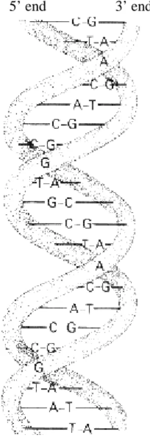
DNA is a linear polymer consisting of the combinations of four different nucleotide bases (here often referred to as bases); deoxyAdenosine monophosphate (abbreviated Adenine or A), deoxyThymidine monophosphate (Thymine or T), deoxyGuanosine monophosphate (Guanine or G) and deoxyCytidine monophosphate (Cytosine or C). DNA sequences do not exist as single sequences of nucleotides (i.e. strands). The strands are wound around each other in opposite directions (i.e. forward and reverse strand) forming a double helix structure held together by hydrogen bounds (Figure 1). All Gs on one strand are paired with Cs on the other strand, while all As are paired with Ts on the opposite strand. This pattern results in an equal amount of A and T, and an equal amount of G and C. (Lewin, 1998, Griffiths et. al., 1996).
As also shown in Figure 1 the DNA strands have directionality. One end of a strand is called the 5’ while the other end is called the 3’end. The two strands in the DNA double helix run in the opposite directions. One chain runs in the 5’→ 3’ direction while the other runs in the 3’→ 5’ direction. More detailed facts about the DNA double helix can be found in (Kleinsmith and Kish, 1995).
Figure 1. A stylized representation of the DNA double helix. The two DNA
strands are held together by hydrogen bounds between Adenine (A) and thymine (T), and between guanine (G) and cytosine (C). The two chains run in opposite directions. One chain runs in the 5’→ 3’ direction while the other runs in the 3’→ 5’ direction.
The relationship between the DNA sequence and the corresponding protein sequence is referred to as the Genetic Code (Lewin, 1997).
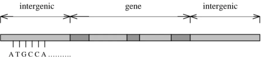
The human DNA consists of genes with intergenic regions in between. These intergenic regions are on average 25-30 kb2. The genes consist of a number of coding regions (i.e. exons) with non-coding regions (i.e. introns) in between. This is shown in Figure 2. The number of exons in a gene is generally correlated with the gene length while the exon length is 170 bases on average and independent of the length of the gene. The length of the introns varies enormously and it seems to have a direct correlation with the length of the gene. These facts are found in Strachan and Read (1996), where more details of the human molecular genetics also can be found. In general the exon/intron boundries are crusial to exon prediction. A basic rule that is used to find exons intron boundries is called the GT-AG-rule, which states that introns virtially always start with GT and end with AG. More about intron exon boundries can be foun in Strachan and Read (1996).
Figure 2. A DNA sequence. Dark gray regions represent exons and light gray
regions represent introns.
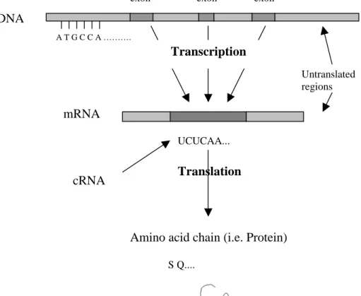
The transcription process that describes the transcription of a gene is shown schematically in Figure 3. Inside the eukaryotic nucleus some genes are active almost
A T G C C A ……….
gene intergenic intergenic
constantly while others have to be turned on and off by specific signals from outside the cell (e.g. some hormone substance) or inside the cell (e.g. a signal from a regulatory gene which turns on and off other genes). These signals bind to specific regions of the gene and initiate the RNA synthesis that makes a copy of the gene’s DNA. In any given region of the DNA sequence only one of the two strands codes for a protein. The copies are single stranded molecules called RNA. RNA is a polymer similar to DNA consisting of Adenosine monophosphate (A), Guanosine monophosphate (G), Cytidine monophosphate (C) and Uridine monophosphate (which is abbreviated U and is functionally equivalent to Thymidine monophosphate) (Griffiths et.al. 1996). The RNA sequence is complementary to the non-coding strand and identical with the coding strand (except that U is used instead of T).
In the process called RNA splicing all introns in the RNA sequence are removed and the resulting mRNA (messenger RNA, transfer RNA or ribosomal RNA) sequence does only contain the coding information (i.e. the exons).
Next, the translation process converts the mRNA nucleotide sequence into amino acid sequence building a protein. The nucleotides in the mRNA sequence are read in triplets (codons), each translated into one amino acid.
2 Kb. Kilo bases. One base is one nucleic acid.
Figure 3. Transcription from DNA to mRNA, and translation from cRNA to
amino acids. The amino acid chain folds up into a protein.
2.2 Gene-finding programs
The laboratory analysis of DNA sequences is difficult, time consuming, and expensive which makes computational techniques essential. The complexity of genes (which is not completely understood) makes hand-coded algorithms impractical (Craven and Shavlink, 1994).
A T G C C A ……….
exon exon exon
Transcription Untranslated regions DNA mRNA Translation cRNA UCUCAA...
Amino acid chain (i.e. Protein) S Q....
Since the 1980s a number of computational methods and approaches have been used to predict protein-coding regions (exons) in genomic DNA sequences. In the early 1990s (Fields and Soderlund, 1990) developed a program, gm, which assembled the coding regions in C. elegans DNA into translatable mRNA sequences. Since then, many different computer based techniques have been tried in this domain; artificial neural networks, hidden Markov models (Henderson et. al. 1997) (Krogh, 1997)(Kulp et. al., 1996) (Kulp and Haussler, 1997), dynamic programming (Salzberg, 1997), dynamic programming and neural networks combined (Snyder and Stormo, 1992) (Snyder and Stormo, 1995). Methods based on homology detection in amino acid sequence databases have also been tried (Rogozin et. al., 1998). Salzberg et. al. (1996) used decision trees and dynamic programming . A method based on a prediction algorithm that uses the quadratic discriminant function for multivariate statistical pattern recognition was used by Zhang (1997).
In this project the three well-known gene-finding programs GRAILII, FEXH, and GENSCAN will be used. The program results will be evaluated separately as well as the combinations of the results.
In the following subchapters (2.5.1, 2.5.2, and 2.5.3) the human DNA sequence D49493 will be used for examples. This sequence is part of the data set used in this project and it is found in GenBank. In Chapter 2.6 GenBank is discussed and the actual structure of D49493 will be shown as the example output from the database. The example sequence used in the three subchapters will illustrate the problem of combining the results from gene-finding programs.
2.2.1 GRAILII
The GRAILII program can be accessed over the web when manually pasting in sequences or through the GRAIL email-server 3. The resulting GRAILII prediction consists of a set of non-overlapping exons in both forward and reverse strand with assigned scores between 0 and 100 to illustrate the quality of the prediction. In this project only the forward strand predictions are considered since not all programs give a prediction on the reverse strand.
GRAILII uses a neural network which recognizes coding regions within variable-size windows tailored to each potential coding region candidate, defined as an open reading frame bounded by a pair of translation start/donor, acceptor/donor, acceptor/translation stop, or translation start/stop sites. The scheme facilitates the use of genomic context information. For more information about GRAILII see Uberbacher and Mural (1991), Uberbacher et. al. (1993), and Mural et.al. (1992).
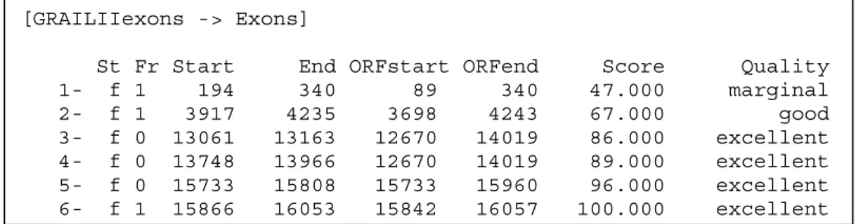
An example of a GRAILII exon prediction is shown in Figure 4. St is the strand the exon is predicted on (f for forward and r for reverse). As mentioned earlier, it is only the forward strand predictions that are considered in this project. Fr is the reading frame. Start and End give the start and end positions (in the sequence) of the predicted exon. There is also a Score associated with the predicted exon which reflects the quality of the prediction. The scores are divided in three quality groups; marginal, good and excellent.
Figure 4. GRAILII prediction for human DNA sequence D49493. The start and
end positions of the predicted exons are given together with a score and quality measure of the prediction. In this particular example there are only forward strand predictions. GRAILII also give reverse strand predictions.
The scores associated with the predictions are normalized between 0.2 and 0.8. 0.2 is a non-predicted nucleotide, while 0.8 corresponds to a nucleotide predicted positive with a score of 100.000. The normalization is explained in Figure 8.
2.2.2 GENSCAN
GENSCAN is developed at the Department of Mathematics at Stanford University California USA4. It is available for academic users over the web.
GENSCAN is a gene-finding program build to analyze DNA sequences from a number of organisms including human. The program is based on a hidden Makrov model.
4
GENSCAN. http://bioweb.pasteur.fr/seqanal/interfaces/genscan.html
[GRAILIIexons -> Exons]
St Fr Start End ORFstart ORFend Score Quality 1- f 1 194 340 89 340 47.000 marginal 2- f 1 3917 4235 3698 4243 67.000 good 3- f 0 13061 13163 12670 14019 86.000 excellent 4- f 0 13748 13966 12670 14019 89.000 excellent 5- f 0 15733 15808 15733 15960 96.000 excellent 6- f 1 15866 16053 15842 16057 100.000 excellent
Using a probabilistic model of the gene’s structural and compositional properties of the genomic DNA for a given organism the program determines the most likely gene structure. The probabilistic model used considers many of the essential gene structural properties of DNA sequences e.g. the typical number of exons per gene, the typical gene density, and the distribution of exon sizes for different types of exons (Burge and Karlin, 1997, Burge 1997).
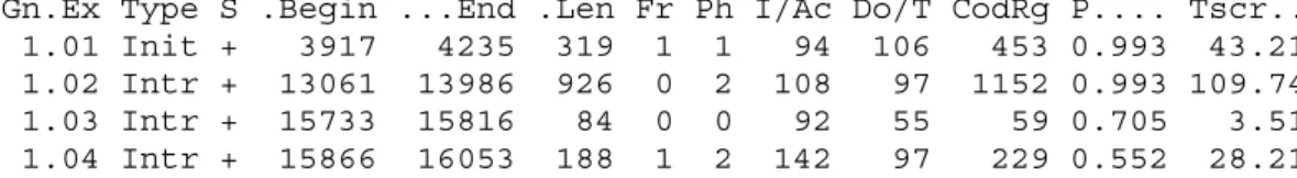
In Figure 5 the GENSCAN prediction of human DNA sequence D49493 is shown. GENSCAN gives the Begin and End positions for the predicted exons. The Type of the predicted exon is also given (Init = Initial exon, Intr = Internal exon, Term = Terminal exon, Sngl = Single-exon gene, Prom = Promoter, PlyA = poly-A signal). The DNA strand on which the predicted exon is located is specified under S (+ for input strand, - for opposite strand). The length (i.e. number of base pairs) of the exon is given under Len. There are a number of other informative measures (i.e. Fr Ph I/Ac Do/T CodRg) that give even more information of the predicted exons but these variables are not considered in this project. Finally GENSCAN gives a quantity (P) that can be considered as the probability of the prediction being correct. The score of the exon (Tscr) is dependent on the Len, I/Ac, Do/T and CodRg scores and is used as an overall measure of the prediction quality.
Figure 5. Output from GENSCAN. The exon prediction of the human DNA
sequence D49493. The information used in this project from this output is the Begin and End positions of the predicted exons and the associated probability P.
The probability assigned to a predicted exon region is normalized between 0.2 and 0.8. A value of 0.2 is a non-predicted nucleotide, while 0.8 correspond to a curtain prediction. The normalization is explained in Figure 8.
2.2.3 FEXH
FEXH was developed at the Department of Cell Biology at Baylor College of Medicine (Solovyev et. al., 1994). In this project FEXH version 2 will be used which was
GENSCAN 1.0 Date run: 20-May-99 Time: 10:53:17
Sequence D49493 : 17286 bp : 51.57% C+G : Isochore 3 (51 - 57 C+G%) Parameter matrix: HumanIso.smat
Predicted genes/exons:
Gn.Ex Type S .Begin ...End .Len Fr Ph I/Ac Do/T CodRg P.... Tscr.. 1.01 Init + 3917 4235 319 1 1 94 106 453 0.993 43.21 1.02 Intr + 13061 13986 926 0 2 108 97 1152 0.993 109.74 1.03 Intr + 15733 15816 84 0 0 92 55 59 0.705 3.51 1.04 Intr + 15866 16053 188 1 2 142 97 229 0.552 28.21 Predicted peptide sequence(s):
>D49493|GENSCAN_predicted_peptide_1|506_aa MAHVPARTSPGPGPQLLLLLLPLFLLLLRDVAGSHRAPAWSALPAAADGLQGDRDLQRHP GDAAATLGPSAQDMVAVHMHRLYEKYSRQGARPGGGNTVRSFRARLEVVDQKAVYFFNLT SMQDSEMILTATFHFYSEPPRWPRALEVLCKPRAKNASGRPLPLGPPTRQHLLFRSLSQN TATQGLLRGAMALAPPPRGLWQAKDISPIVKAARRDGELLLSAQLDSEERDPGVPRPSPY APYILVYANDLAISEPNSVAVTLQRYDPFPAGDPEPRAAPNNSADPRVRRAAQATGPLQD NELPGLDERPPRAHAQHFHKHQLWPSPFRALKPRPGRKDRRKKGQEVFMAASQVLDFDEK TMQKARRKQWDEPRVCSRRYLKVDFADIGWNEWIISPKSFDAYYCAGACEFPMPKVDAYS VASAGEQQQSSMAWDCEDGMGAWIVRPSNHATIQSIVRAVGIIPGIPEPCCVPDKMNSLG VLFLDENRNVVLKVYPNMSVDTCACX
released in May 1994. The department has released newer and more accurate programs since then, but this version will be used to keep the similarity to the experiments done by Murakami and Takagi (1998) as high as possible. FEXH is available through WWW and as an e-mail service5.
The algorithm FEXH used to predict exons is briefly described in two steps. Firstly, all internal exons in the sequence are predicted using a linear discriminant function that combines the characteristics that describe donor and acceptor splice sites, 5’-and 3’-intron regions and also the coding region for each open reading frame flanked by GT and AG base pairs. Then, the potential 5’-and 3’-exons are predicted by discriminant functions on the left side of the first internal exon and on the right side of the last internal exon.
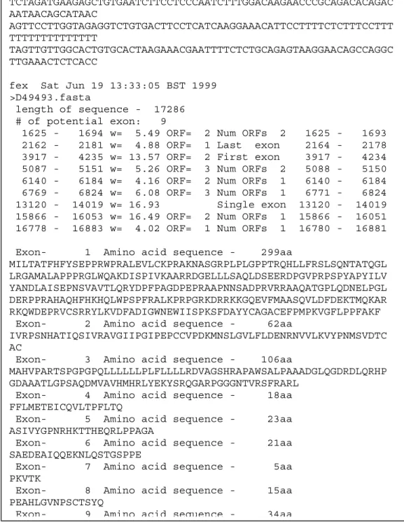
In Figure 6 the FEXH exon prediction for the human DNA sequence D49493 is shown. Start and end positions of the predicted exons are given together with weights (w) that reflect the prediction certainty. The information about open reading frames (ORF) is not used in this project. For more details see Solovyev and Salamov (1997) and Solovyev et.al. (1994).
Figure 6. FEXH prediction of the human DNA sequence D49493. The predicted
exons are given start and end positions in the sequence and an associated weight which reflects the quality of the prediction.
Name: D49493.fasta
First three lines of sequence:
TCTAGATGAAGAGCTGTGAATCTTCCTCCCAATCTTTGGACAAGAACCCGCAGACACAGAC AATAACAGCATAAC AGTTCCTTGGTAGAGGTCTGTGACTTCCTCATCAAGGAAACATTCCTTTTCTCTTTCCTTT TTTTTTTTTTTTTT TAGTTGTTGGCACTGTGCACTAAGAAACGAATTTTCTCTGCAGAGTAAGGAACAGCCAGGC TTGAAACTCTCACC
fex Sat Jun 19 13:33:05 BST 1999
>D49493.fasta length of sequence - 17286
# of potential exon: 9
1625 - 1694 w= 5.49 ORF= 2 Num ORFs 2 1625 - 1693 2162 - 2181 w= 4.88 ORF= 1 Last exon 2164 - 2178 3917 - 4235 w= 13.57 ORF= 2 First exon 3917 - 4234 5087 - 5151 w= 5.26 ORF= 3 Num ORFs 2 5088 - 5150 6140 - 6184 w= 4.16 ORF= 2 Num ORFs 1 6140 - 6184 6769 - 6824 w= 6.08 ORF= 3 Num ORFs 1 6771 - 6824 13120 - 14019 w= 16.93 Single exon 13120 - 14019 15866 - 16053 w= 16.49 ORF= 2 Num ORFs 1 15866 - 16051 16778 - 16883 w= 4.02 ORF= 1 Num ORFs 1 16780 - 16881 Exon- 1 Amino acid sequence - 299aa
MILTATFHFYSEPPRWPRALEVLCKPRAKNASGRPLPLGPPTRQHLLFRSLSQNTATQGL LRGAMALAPPPRGLWQAKDISPIVKAARRDGELLLSAQLDSEERDPGVPRPSPYAPYILV YANDLAISEPNSVAVTLQRYDPFPAGDPEPRAAPNNSADPRVRRAAQATGPLQDNELPGL DERPPRAHAQHFHKHQLWPSPFRALKPRPGRKDRRKKGQEVFMAASQVLDFDEKTMQKAR RKQWDEPRVCSRRYLKVDFADIGWNEWIISPKSFDAYYCAGACEFPMPKVGFLPPFAKF Exon- 2 Amino acid sequence - 62aa
IVRPSNHATIQSIVRAVGIIPGIPEPCCVPDKMNSLGVLFLDENRNVVLKVYPNMSVDTC AC
Exon- 3 Amino acid sequence - 106aa
MAHVPARTSPGPGPQLLLLLLPLFLLLLRDVAGSHRAPAWSALPAAADGLQGDRDLQRHP GDAAATLGPSAQDMVAVHMHRLYEKYSRQGARPGGGNTVRSFRARL
Exon- 4 Amino acid sequence - 18aa FFLMETEICQVLTPFLTQ
Exon- 5 Amino acid sequence - 23aa ASIVYGPNRHKTTHEQRLPPAGA
Exon- 6 Amino acid sequence - 21aa SAEDEAIQQEKNLQSTGSPPE
Exon- 7 Amino acid sequence - 5aa PKVTK
Exon- 8 Amino acid sequence - 15aa PEAHLGVNPSCTSYQ
In this project the by FEXH predicted exon-regions are coded using the weight associated with the predictions. The weight is a linear discriminant value that might be any, but in practice the weights are around 0. –10 and +100 are probably the limits. (Solovyev et.al. 1994) . To normalize the weights between 0.2 and 0.8 the standard deviation was computed on the whole data set. The format of the predictions after normalization is shown in Figure 8.
2.3 GenBank
GenBank is a database containing nucleic acid sequences gathered from patents and journal literature and direct author submissions. The producer of the database is the National Center for Biotechnology Information, USA 6. GenBank is updated daily and reloaded weakly.
The nucleic acid sequences contained in GenBank have related descriptive information such as source organism, description, sequence length, and references.
For all the sequence in the data set the information about exons in GenBank will be used as the actual exons. In the data files the CDS will be used as in Murakami and Takagi’s (1998) experiments.
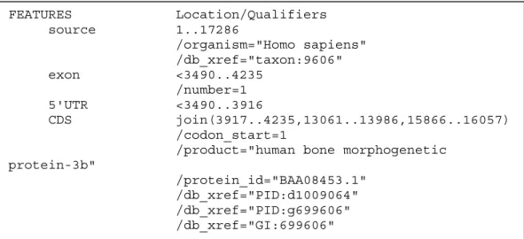
In Figure 7 the GenBank entry for the human DNA sequence D49493 is shown. It is only a small part of the file. The complete file can be seen in appendix A. The CDS-regions marked in the file can be compared to the predictions made by the separate programs on the same sequence (see Chapter 2.2). This exemplifies the problem of combining the different predictions to gain the best overall prediction.
Figure 7. A part of the GenBank entry for the human DNA sequence D49493.
The regions marked by CDS are used as actual exons.
6
National Center for Biotechnology Information, 8600 Rockville Pike, Bethesda, MD 20892, USA.
FEATURES Location/Qualifiers source 1..17286 /organism="Homo sapiens" /db_xref="taxon:9606" exon <3490..4235 /number=1 5'UTR <3490..3916 CDS join(3917..4235,13061..13986,15866..16057) /codon_start=1
/product="human bone morphogenetic protein-3b" /protein_id="BAA08453.1" /db_xref="PID:d1009064" /db_xref="PID:g699606" /db_xref="GI:699606" /translation="MAHVPARTSPGPGPQLLLLLLPLFLLLLRDVAGSHRAPAWSALP AAADGLQGDRDLQRHPGDAAATLGPSAQDMVAVHMHRLYEKYSRQGARPGGGNTVRSF RARLEVVDQKAVYFFNLTSMQDSEMILTATFHFYSEPPRWPRALEVLCKPRAKNASGR PLPLGPPTRQHLLFRSLSQNTATQGLLRGAMALAPPPRGLWQAKDISPIVKAARRDGE LLLSAQLDSEERDPGVPRPSPYAPYILVYANDLAISEPNSVAVTLQRYDPFPAGDPEP RAAPNNSADPRVRRAAQATGPLQDNELPGLDERPPRAHAQHFHKHQLWPSPFRALKPR PGRKDRRKKGQEVFMAASQVLDFDEKTMQKARRKQWDEPRVCSRRYLKVDFADIGWNE WIISPKSFDAYYCAGACEFPMPKIVRPSNHATIQSIVRAVGIIPGIPEPCCVPDKMNS LGVLFLDENRNVVLKVYPNMSVDTCACR" intron 4236..13060 /number=1 exon 13061..13986 /number=2 intron 13987..15865 /number=2 exon 15866..>16827 /number=3 3'UTR 16058..>16827 polyA_signal 16810..16815
The predicted exon regions are assigned the score 0.8, while all other nucleotides have the value 0.2. This is shown in Figure 8.
2.4 Combination of results from gene-finding programs
Many researchers have discussed the unsatisfying results of most gene-finding programs available today (e.g. Rogozin et. al., 1998). Burset and Guigó (1996) state on page 355 in their article:
Thus, although the current generation of programs may still be of great use in pinpointing some of the regions containing exons in large DNA genomic sequences, the programs are unlikely to be able, in most cases, to elucidate their genomic structure completely.
Burset and Guigó (1996) discussed the possible advantages of combining gene-finding program results. The initial experiment results they presented suggested that a combination of gene-finding programs might be useful if an appropriate combination method is found.
In a review in Trend in Genetics in August 1996 James Fickett discussed the state of the art of gene-finding programs and how working principles and strengths of different programs (methods or algorithms) could be combined to gain the optimum gene identification accuracy. Fickett suggested development of a framework for program integration allowing users to integrate any set of programs.
One of the first attempts to combine results from several gene-finding programs was made by Murakami and Takagi (1998). They tested four different gene-finding programs; FEXH, GeneParser3, GENSCAN, and GRAILII. The results from the programs were combined using the five methods AND, OR, HIGHEST, RULE and BOUNDARY (see Chapter 1 for description of the methods) and the results were evaluated.
The human DNA sequences in their data set were collected from GenBank release 100 (April 1997), using a number of selection criteria described in Chapter 3.2. In the article Murakami and Takagi (1998) criticize earlier gene-finding program evaluations which were done using data sets that were not sufficiently documented. The training set and test set used are not always clearly defined e.g. there might be sequences in test sets that are very similar to sequences used in training set. The uncareful selection of sequences in the dataset might be the explanation why tests done by program developers show clearly better results than the test done by Murakami and Takagi (1998).
The results presented in the article (Murakami and Takagi, 1998) showed that by two of the methods the approximate correlation (see Chapter 3.3 for definition) was improved by 3-5 % in comparison with the best single gene-finding program (GENSCAN) tested. The methods OR, HIGHEST and BOUNDARY show increasing accuracy as the number of gene- finding programs increase. The accuracy decreases as the number of programs combined increase with the AND method. The tests show that one program, GENSCAN, has an accuracy that is difficult to increase by combining the program with any of the other three programs (FEXH, GRAIL and GeneParser3).
The experiments results presented in the article by Murakami and Takagi (1998) inspired the work in this project. As stated in the thesis statement in Chapter 1 three new methods for combination of gene-finding programs are evaluated in this project. Two of the methods are based on ANNs and they are expected to perform better than the logical methods AND, OR, and MAJ.
2.5 Chapter summary
In this Chapter the background for the project is outlined briefly. The necessary biological background is described to introduce the reader to the problem domain. It is important to understand the distinction between DNA, genes, exons, and introns. There are also facts about the DNA that will give the reader an understanding of the complexity in gene-searching.
Many different computer based techniques have been tried for the gene-searching problem. In this Chapter some techniques are presented and there are references to a number of researchers using different techniques. The three well-known gene-finding programs used in this project are presented (i.e. GRAILII, FEXH, and GENSCAN). GenBank, the enormous database of DNA sequences is briefly introduced to the reader. It is the exons in GenBank files of the sequences in the data set that will be used as the actual exons.
Researchers that have discussed the advantages of combining results from gene-finding programs are presented. The key background for this project is the article published by
Murakami and Takagi (1998). Results of the evaluation of methods for combining gene-finding program results are discussed.
The chapter in its whole illustrates the motivation for the aim and hypothesis addressed in this project.
3 Experiments
The aim of this project is to compare different methods for combining results from gene-finding programs. The experiments that are performed within this project are presented in this Chapter.
In addition to the logical combination methods inspired by Murakami and Takagi (1998) this project includes the use of ANNs to combine the results of the gene-predicting programs. Two types of ANNs will be used; basic feed-forward neural networks and feed-forward neural networks using sliding windows.
3.1 Overview of experiments
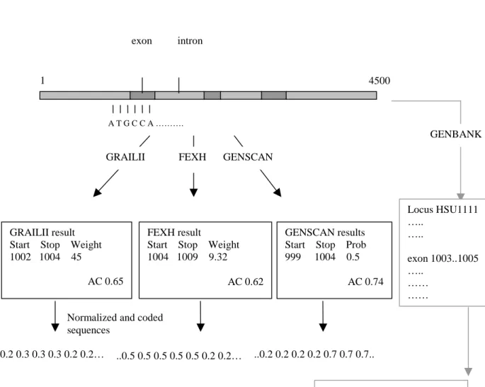
The process through which the hypothesis will be fulfilled or falsified is show in Figures 8 and 9.
Normalized and coded sequences
..0.2 0.2 0.3 0.3 0.3 0.2 0.2…
1 4500
Figure 8. The first steps in the process of this project. For explanation see the
text.
All sequences in the data set are analyzed by all the gene-finding programs used in this project (i.e. GRAILII, FEXH and GENSCAN). In Figure 8 there are examples of the output from the programs. All three programs give the results in this form (See Chapter 2.2). The start and the stop positions for a predicted exon are given with a weight,
GENBANK
DNA sequence
GRAILII result Start Stop Weight 1002 1004 45
AC 0.65
A T G C C A ……….
GRAILII FEXH GENSCAN
FEXH result
Start Stop Weight 1004 1009 9.32
AC 0.62
GENSCAN results Start Stop Prob 999 1004 0.5 AC 0.74 Locus HSU1111 ….. ….. exon 1003..1005 ….. …… …… .. 0.2 0.2 0.2 0.8 0.8 0.8 0.2… ..0.5 0.5 0.5 0.5 0.5 0.2 0.2… ..0.2 0.2 0.2 0.2 0.7 0.7 0.7.. exon intron
score, or probability to illustrate the probability of the prediction being correct. The predicted sequence structures are built using these outputs normalized between 0.2 and 0.8 (this is just to give the ANN a more manageable scale of inputs). To the right in the figure the correct sequence structure is fetched from GenBank. The actual sequence structure is encoded in the same way as the predicted structures. The minimum value (i.e. 0.2) is used for all non-coding nucleotides and the maximum value (i.e. 0.8) is used for positions with true coding nucleotides. The rest of the process is illustrated in Figure 9.
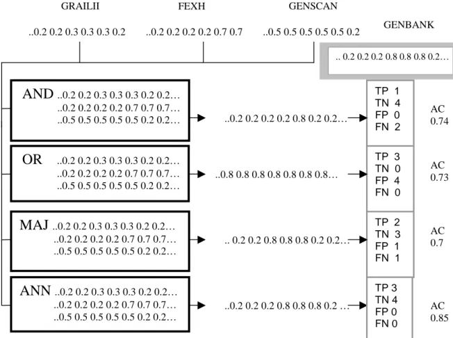
Figure 9. The steps of the project process where the results from different
exon-predicting programs are combined using different methods. This process is explained in detail in the text.
The sequences are combined using the four different methods (i.e. AND, OR, MAJ, ANN). With the AND method all program predictions need to be positive (i.e. greater than 0.2 that represent negative, non-coding regions) at a certain position in the sequence for the overall prediction to be positive. With the OR method only one of the predictions at a certain position needs to be positive for the resulting prediction at that position to be positive. The MAJ method needs at least two
.. 0.2 0.2 0.2 0.8 0.8 0.8 0.2… AC 0.74 AC 0.73
AND
..0.2 0.2 0.3 0.3 0.3 0.2 0.2… ..0.2 0.2 0.2 0.2 0.7 0.7 0.7… ..0.5 0.5 0.5 0.5 0.5 0.2 0.2…OR
..0.2 0.2 0.3 0.3 0.3 0.2 0.2… ..0.2 0.2 0.2 0.2 0.7 0.7 0.7… ..0.5 0.5 0.5 0.5 0.5 0.2 0.2…MAJ
..0.2 0.2 0.3 0.3 0.3 0.2 0.2… ..0.2 0.2 0.2 0.2 0.7 0.7 0.7… ..0.5 0.5 0.5 0.5 0.5 0.2 0.2…ANN
..0.2 0.2 0.3 0.3 0.3 0.2 0.2… ..0.2 0.2 0.2 0.2 0.7 0.7 0.7… ..0.5 0.5 0.5 0.5 0.5 0.2 0.2… ..0.2 0.2 0.2 0.2 0.8 0.2 0.2… ..0.8 0.8 0.8 0.8 0.8 0.8 0.8… .. 0.2 0.2 0.8 0.8 0.8 0.2 0.2… ..0.2 0.2 0.2 0.8 0.8 0.8 0.2 … TP 1 TN 4 FP 0 FN 2 TP 3 TN 0 FP 4 FN 0 TP 2 TN 3 FP 1 FN 1 AC 0.7 7 AC 0.85 ..0.5 0.5 0.5 0.5 0.5 0.2 ..0.2 0.2 0.3 0.3 0.3 0.2 ..0.2 0.2 0.2 0.2 0.7 0.7GRAILII FEXH GENSCAN
GENBANK
TP 3 TN 4 FP 0 FN 0
programs to give a positive prediction for the overall prediction to be positive. The ANN might adopt a strategy in between the other methods.
The resulting predictions after combining the individual program predictions are compared to the sequence structure found in GenBank. To calculate the accuracy on the exon level every position of the predicted sequence structure is compared to the true sequence structure. The number of True Positives (TP) is calculated which shows the number of correctly predicted positives. The number of correctly predicted negatives, called True Negatives (TN), is calculated. The False Positives (FP) are the incorrectly predicted positive and the False Negatives (FN) are the incorrectly predicted negative. The variables are used to calculate the Approximate Correlation (AC) (i.e. the association between prediction and reality) and other measures used to illustrate the accuracy of the prediction. (See Chapter 3.3).
In the Figure 8 example AC values are given for the programs when used separately on the data set in this project. Example values of AC after using the combination methods are shown in Figure 9. Murakami and Takagi (1998) showed that in general the AC was improved by a combination of programs. The AND and OR methods used here are inspired by Murakami and Takagi’s (1998) experiments.
3.2 Data set
The data set Murakami and Takagi (1998) chose for their project will be used in this project. The criteria they used when choosing DNA sequences from GeneBank are well documented (see Figure 10) and using the same data set will contribute to a possible comparison between results in the projects, see discussion in Chapter 9.
Figure 10. The criteria for loci selection from GenBank used by (Murakami et al,
1998).
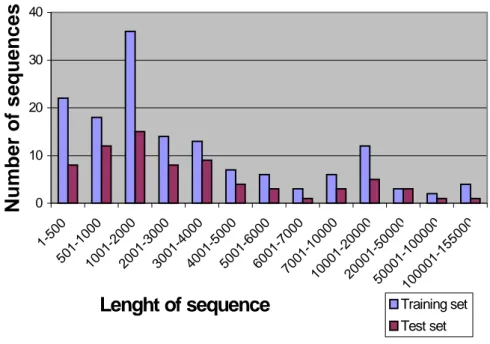
The process of collecting sequences from GenBank resulted in a data set of 219 loci7 that were randomly divided in two parts; training set and test set. The training set consists of two thirds of the data set (146 loci) and the test set consists of the remaining third (73 loci). These data sets are available upon request from Murakami and Takagi (1998). In appendix A there is a list of all 219 loci with name and sequence length.
The lengths of the sequences are spread over a spectrum as the graph shows in Figure 11.
7
Loci. Pl. For locus. Locus is an accession number of ensured unikeness in GenBank.
From GenBank Release 100 (April 1997) (Murakami et. al., 1998) collected loci that meet these criterias:
• Human DNA sequences with at least one ‘CDS’ • ‘SOURCE’ is Homo sapiens
• standard splice site conservative dinucleotides (i. e. GT-AC) • confirmed experimentally to be transcribed
• immunoglobin genes discarded due to the complexity of their
structure
• registrated after June 1996
• do not code for proteins that are homologous to already known
Figure 11. The lengths of the sequences in the training set and test set. Note
that the ranges of sequence lengths are different.
3.3 Performance measures
The accuracy of the predictions of gene-finding programs is often measured at three different levels; nucleotide level, exon level, and protein product level (Burset and Guigó, 1996). At the coding nucleotide level the prediction accuracy is measured by comparing the prediction (coding or non-coding nucleotide) with the actual nucleotide value (coding or non-coding) for each nucleotide separately along the sequence. At the exon level the accuracy of the prediction is measured by comparing the predicted exons with the actual exons along the sequence. An exon that is correctly predicted is generally defined as an exact match with the true exon (i.e. has to include both the start
DNA sequences
0 10 20 30 40 1-50 0 501-10 00 1001-20 00 2001-30 00 3001-40 00 4001-50 00 5001-60 00 6001-70 00 7001-100 00 10001-200 00 20001-500 00 50001-1000 00 100001-1550 00 Lenght of sequence N umber of sequence s Training set Test set
and the stop codon). The accuracy of predictions measured at the protein product level is performed by comparing the protein product encoded by the predicted gene with the protein product encoded by the actual gene. This approach gives a measure of how well the predicted exons assemble into the correct protein product. High similarity between such a predicted protein product and a known protein sequence may improve the prediction.
In this project only prediction accuracy at the nucleotide and exon levels is considered. There are four well recognized measures of performance used when evaluating gene-predicting programs; Sensitivity, Specificity, Correlation Coefficient and Approximate Correlation. The measures are used in other areas as well (e.g. protein folding prediction (Sternberg, 1997)). The measures are explained in more detail in the following subchapters. These measures are commonly used and they are also used in this project for comparison reason. There are some problems associated with the measures however, and these are discussed in the following subchapters.
3.3.1 Nucleotide level
A common approach to measure prediction accuracy is at the nucleotide level (see e.g. Murakami and Takagi, 1998, Burset and Guigó, 1996). The actual nucleotide value as well as the predicted nucleotide value can be either coding or non-coding (positive or negative) and associations between the prediction value and the actual value have been widely used as measures of prediction accuracy. The values (coding or not) of the real DNA sequence compared to the values in the prediction are shown in Figure 12. The top square in Figure 12 represents the nucleotides of the DNA sequence to be analyzed. These are divided in two groups; actual positives and actual negatives. The square in
the middle represents possible outputs from a gene-finding program. The gene-finding program does not give 100% correct predictions. Most of the actual positive nucleotides are predicted as being positives and most of the actual negatives are predicted negative. There are some actual negative nucleotides that are predicted as positives, as well as there are some actual positives predicted as negatives. When comparing the predicted values of the nucleotides with the actual values, the result is a number of correct positive predictions (True Positives or TP), and a number of correct negative predictions (True Negatives or TN). The comparison between the prediction and the actual sequence also results in a number of incorrectly positive predictions (False Positives or FP), and a number of incorrectly negative predictions (False Negatives or FN). The results of the comparison in this example are shown in the bottom square in Figure 12.
Figure 12. The variables used when evaluating a predicted DNA sequence
structure. The top sequence shows the actual DNA sequence structure. For simplicity this sequence has only one non-coding region (intron) followed by one coding region (exon). The middle sequence illustrates the prediction of the DNA sequence structure. The dark regions are regions of predicted coding bases and the light regions are regions of predicted non-coding bases. The bottom sequence shows the result of the comparison of the predicted DNA sequence structure with the actual sequence structure. For every nucleotide base, the prediction is compared to the actual nucleotide base at the corresponding position in the actual sequence. For the whole sequence the total number of correctly predicted positives (i.e. True Positives), the correctly predicted negatives (i.e. True Negatives), the incorrectly predicted positives (i.e. False Positives), and the incorrectly predicted negatives (i.e. False Negatives), are counted.
The associations between the four variables (TP, TN, FP, FN) are often derived by the two measures; Sensitivity (Sn) and Specificity (Sp), which are defined in definition 1.
Actual negatives (noncoding) Actual positives (coding)
Predicted positives Pred. Pos. Predicted Negative
FN FN False Pos. True Positives Pred Neg.
Actual positives (coding) DNA
Predicted structure
Prediction evaluation
Sn is the proportion of predicted positive nucleotides actually being positives, while Sp is the proportion of actual positive nucleotides being predicted as positives.
)
(
TP
FN
TP
Sn
+
=
)
(
TP
FP
TP
Sp
+
=
Definition 1. The definitions of sensitivity (Sn) and Specificity (Sp).
Sensitivity is the proportion of coding nucleotides correctly predicted as coding. The specificity is the proportion of non-coding nucleotides correctly predicted as non-coding.
It is obvious that a prediction of a gene-predicting program can result in high sensitivity but very low specificity (e.g. when the program predicts all nucleotides to be positive when they are actually not) as well as high specificity together with very low sensitivity (e.g. the program predicts all nucleotides as negatives when there are a number of actual positives). The sensitivity and specificity measures do not reflect the size of the data set. The measures used separately do not give a good picture of the prediction accuracy.
Correlation Coefficient (CC) is a measure widely used for evaluation of the gene-prediction accuracy. CC ranges fro –1 to 1 and reflects the association between the prediction and the reality. Definition 2 gives the formal definition of CC. CC is an appropriate measure of the overall prediction accuracy since it depends on both the
sensitivity and specificity in predicting positive nucleotides, as well as sensitivity and specificity in predicting negative nucleotides.
CC has one drawback. In situations were the prediction or the reality does not contain either any positives or any negatives. CC is not defined for situations when TP+FN, TP+FP, TN+FP, or TN+FN is zero.
))
(
)
(
)
(
)
((
))
(
)
((
FN
TN
FP
TN
FP
TP
FN
TP
FP
FN
TN
TP
CC
+
×
+
×
+
×
+
×
−
×
=
Definition 2. Correlation Coefficient (CC).
Approximate correlation (AC) is also a widely used accuracy measure. It is defined in definition 3. AC ranges from –1 to 1 and appears to be an approximation of CC. It can therefore be used as an alternative to CC. (Burset and Guigo, 1996).
1
2
1
+
+
+
−
=
⎥ ⎥ ⎦ ⎤ ⎢ ⎢ ⎣ ⎡PN
TN
AN
TN
PP
TP
AP
TP
AC
Definition 3. Approximate Correlation (AC). AC shows the association between
3.3.2 Exon level
When measuring accuracy at the exon level the comparison between the prediction and the reality with regard to the complete exons (Figure 13). The top square in Figure 13 represents the actual structure of the DNA sequence to be analyzed. In the middle square the results from a gene-finding program are shown. The predicted exons do not match exactly with the actual exons in the DNA sequence. To be considered in the accuracy measures the predicted exon has to match exactly with the actual exon. The bottom square shows the correct predicted exon along with a missing exon (M) and a wrong exon. A missing exon is defined as an actual exon not being overlapped with a predicted exon, while a wrong exon is a predicted exon that does not actually exist.
At the exon level the definition for sensitivity (definition 4) is interpreted as the proportion of actual exons being predicted. Specificity (definition 4) is the proportion of predicted exons that are actual exons.
Burset and Guigo (1996) used two additional measures of sensitivity and specificity to compensate for the stringent definition they used for correct exons. Missing Exon (ME) is a measure of the proportion of actual exons with no overlap to the predicted exons. Wrong Exon is the proportion of predicted exons with no overlap to any actual exon. The definitions for these measures are shown in definition 5.
Figure 13. Variables used for accuracy measures at the exon level. In the top
sequence the actual DNA sequence structure is illustrated. The dark gray regions represent the actual exons and the light gray regions represent the actual introns. The middle sequence shows a possible prediction of the sequence structure (or a resulting prediction after combining the results of different programs). The bottom sequence shows the result of the evaluation of the exon prediction. There is one exon predicted with an overlap to an actual exon. The letter symbol CE (i.e. correct exon) represents the exon that has been predicted exactly. The variables that will be used for accuracy measures at the exon level are the missing exons (i.e. ME) and the wrong exons (i.e. WE). A missing exon is an actual exon that has no overlap in any predicted exon. A wrong exon is a predicted exon that has no overlap in any actual exon.
1 2 1 CE WE 2 3 3 ME DNA Prediction Prediction evaluation
Exons
Actual
of
Number
Exons
Correct
of
Number
=
Sn
Exons
Predicted
of
Number
Exons
Correct
of
Number
=
Sp
Definition 4. Sensitivity (Sn) and Specificity (Sp) at the exon level.
Exons
Actual
of
Number
Exons
Missing
of
Number
=
ME
Exons
Predicted
of
Number
Exons
Wrong
of
Number
=
WE
Definition 5. Missing exons (ME) and wrong exons (WE) at the exon level
In this project the accuracy of the predictions is measured using the measures as defined above. The results from the different gene-finding programs are analyzed separately as well as the combinations of the program predictions. A number of additional measures are found in the literature. See Burset and Guigo (1996) for a deeper analysis of the different measurements.
3.4 AND
One of the simplest ways of combining results from any programs like the ones used here is to use an AND operator. At the nucleotide level this means that an overall positively predicted nucleotide is only considered if all participating programs predict the nucleotide as positive. At the exon level a whole exon has to be predicted by all programs to result in
an overall positive prediction of the exon. How this combination method works at the different levels is shown in Figure 14.
Figure 14. The AND method for combination of gene-predictions. DNA is the
actual sequence being analyzed. P1, P2 and P3 show possible predictions by the different programs. The dark regions represent exons and the light gray regions are introns. . OP is the resulting overall prediction and the result at the nucleotide level. ELR is the result after evaluating the overall prediction at the exon level.
The AND method for combination of results from gene-finding programs was used by Murakami and Takagi (1998). The results obtained in this project are compared to the results presented in their article. There is a difference between how Murakami and Takagi (1998) used the output from the gene-finding programs and how the scores are used here. They transformed the scores of the predicted exons given by the different programs to probabilistic ones. The reason they give for the transformation of scores is that they wanted to be able to compare the quality of the predictions from different programs. The transformation was done by examining the relationship between the scores and the
DNA P1 P2 P3 ELR OP
accuracy of the programs (Murakami and Takagi, 1998). This demands some consideration, for instance when adding a new program to the AND method. Most gene-finding programs have their own way of computing the score, weight or probability of their predictions which might result in difficulty when transforming the predictions to comparable probabilities.
In this project the weights, scores and probabilities given by the different programs with the predictions will be normalized to facilitate use of this data as input to the ANN.
The results from the AND method will also be compared to the results obtained by the different gene-finding programs separately.
The AND method is expected to result in low sensitivity and high specificity, as understandable and as shown by Murakami and Takagi (1998). The sensitivity will generally stay the same or most likely decrease as the number of combined programs increases. Because the method needs a positive prediction by all the programs to give an overall positive prediction, all participating programs have to recognize the same particularities that unveil exons in the sequence. Since each program considers the features of the sequences differently the predictions are often not identical and one program might grasp some features of a gene that others do not (Murakami and Takagi, 1998). The possibility of gaining the advantages from different approaches was the motivation for the idea to combine gene-finding programs based on different techniques. The AND method does not take this program-unique gene-feature recognition into account.
The three possible combinations of two programs among the three programs will be analyzed as well as the combination of all three programs.
3.5 OR
In Figure 15 the method is shown for the nucleotide and exon levels. For an overall positive prediction of a nucleotide there has to be at least one program predicting the nucleotide as positive. In the same way an exon has to be predicted by at least one program to be considered in the overall positive prediction.
Figure 15. The OR method for combination of predictions. DNA is the actual
DNA sequence. P1, P2, and P3 are possible predicted structures of the DNA sequence performed by programs. Dark gray regions represent exons, while light gray regions represent introns. OP is the overall prediction after combining P1, P2, and P3 using the OR method and it is also the resulting prediction at the nucleotide level. ELP is the resulting exons at the exon level.
This combination method was also used by Murakami and Takagi (1998). The results obtained by the experiments in this project will be compared to the results presented in
DNA P1 P2 P3 ELP OP
the article (Murakami and Takagi, 1998). The results obtained by the different programs when used separately will also be compared to Murakami and Takagi’s (1998) results. There will also be a comparison between the different methods for combination of predictions included in this project.
The OR method is expected to consider all exons/nucleotides predicted by the programs. The method will result in low specificity and high sensitivity. A nucleotide/exon predicted as negative is more likely to be actually negative with this method than with AND. The probability that a positive prediction matches an actual positive nucleotide/exon is lower with this method than with AND. The OR method considers all program-unique gene-feature recognitions there are among the combined programs, but it also includes all the programs-unique weaknesses too (e.g. incorrect predictions in situations recognized as coding by a program). The sensitivity is likely to increase as the number of programs increases, while the specificity will decrease as the number of combined programs increases.
The test setups are the same as for the AND method. All possible combinations of two programs among the three will be tested as well as the combination of all three programs.
3.6 Majority
The AND method only considers the nucleotides/exons which are predicted similarly by all the programs, while the OR method considers all the predictions done by the programs. MAJORITY (MAJ) is a method which considers the predictions done similarly by the majority of the programs (i.e. by at least two programs).
The expected results for this method is a sensitivity and a specificity between those of AND and OR. MAJ might result in a higher overall accuracy, AC, when compared to the AND and OR methods of combining three programs.
The MAJ method is tested on only one combination of all three programs (i.e. GRAILII, GENSCAN, and FEXH). Since the MAJ method implies that more than 50% of the programs predict an exon the method is only applicable on an odd number of programs.
3.7 ANN
An artificial neural network (ANN) is a way of learning a function using a network of simple arithmetic computing elements and example data. For a full explanation of the details of ANNs see for instance Russell and Norvig (1995).
The results from the gene-finding programs are predictions of where in the DNA sequence there are coding nucleotides (i.e. possible exons). These exon predictions are assigned scores, weights or probabilities (here referred to as scores) by the different programs reflecting the certainty of the prediction being correct. These scores will be normalized on a scale between 0.2 and 0.8 to encourage sensitivity in the ANN.
The output from the ANN is an overall prediction of every nucleotide along the sequence being coded or not.
Two variants of presenting input data to the ANN are tested. Both variants are simple feed-forward networks. The first ANN (ANN type 1) is given as input one position of a
time along the sequence. ANN type 2 is given as input the nucleotide position at interest as well as the close neighborhood on both sides in the sequence (ANN type 2).
The network configurations are shown in Table 1 in Chapter 3.7.3.
3.7.1 ANN type 1
The topology of the ANN type 1 is shown in Figure 16. The prediction results from the different programs are coded as described in Chapter 3.1 and fed into the network nucleotide by nucleotide. There is one input node for each of the participating programs. The pedictions of the nucleotide sequences are fead into the network one nucleotide at the time. The output from the network is the overall prediction of the nucleotides, one at the time. A threshold is used to divide the output into the two classed predicted positive or predicted negative. Initially the threshold is set to 0.5. The idea is that the ANN should learn which combinations of scores from the different programs that reflect actual coding nucleotides.
GRAILII FEXH GENSCAN
Figure 16. The topology of the ANN type 1. In the figure the ANN combines
results from three programs. A threshold is set to divide the output from the ANN (i.e. predicted coding or predicted non-coding) and decide the overall prediction for every nucleotide along the sequence.
3.7.2 ANN type 2
The inputs are presented to the ANN using a sliding window. The principle of this is shown in Figure 17. It is not only the nucleotide of current interest (i.e. the nucleotide to be predicted) that is presented to the ANN. Four nucleotide predictions before and four nucleotide predictions after the nucleotide of interest are also included in the input. Three windows of nine nucleotides in the sequence (i.e. one window from each program) are fed into the ANN. The ANN will combine the predictions in the windows and give a resulting overall prediction for the nucleotide in the middle. Using this technique the ANN will have more information about the environment (i.e. the neighbor nucleotides). 0.2 0.2 0.2 0.2 0.3 0.7 0.5 0.3 0.7 0.5 0.3 0.7 0.5 0.2 0.7 INPUT OUTPUT
. .
0.2 0.59 0.78 0.79 0.43. .
HIDDENGRAILII INPUT 0.2 0.2 0.5 0.5 0.5 0.3 0.3 0.3 0.2 0.2 0.3 0.3 0.3 0.2 0.2 0.2 0.2 0.2 0.2 0.7 0.7 0.7 0.7 0.7 0.7 0.7 0.7 Fully connected HIDDEN
Figure 17. The ANN type 2 network in the figure is fully connected. The ANN
combines the results from the gene-finding programs. Predictions at every position (i.e. nucleotide) in the sequence are presented to the ANN together with four nucleotides on each side. The output from the ANN is the overall prediction of the nucleotide in the middle of the windows being coded or not (i.e. GRAILII (0.5), FEXH (0.2), and GENSCAN (0.7)). The windows are sliding one position at the time for every position along the sequence making a new input example for the ANN.
3.7.3 Test setup
The test setup for the ANN type 2 is shown in Table 1. The symbol GR stands for GRAILII, FE stand for FEXH and GS is GENSCAN. The tests are run using Matlab Neural Network Toolbox and the training will continue until the minimum error is
OUTPUT
FEXH GENSCAN