SKI Report 01:44
Recharge-area Nuclear Waste Repository
in Southeastern Sweden
Demonstration of Hydrogeologic Siting Concepts
and Techniques
Clifford I. Voss
Alden M. Provost
November 2001
Research
SKI perspective
Background and objective
An important issue in the site selection process are a recharge area (generally an inland location) vs. a discharge area (generally a coastal location). According to SKI, this problem has not yet been thoroughly investigated by SKB, and consequently SKI initiated the present research project to clarify the implications of this factor.
Results
The results from this study indicate that, if dilution mechanisms are disregarded, it may be advantageous to site the repository in a recharge area since one thus may expect longer pathways and travel times through the geosphere. This in turn, implies more time for radioactive decay as well as other retardation mechanisms.
To achieve such long paths and travel times, radionuclide transport need to take place along regional flow paths. Local scale variations in the topography, combined with the fractures and fracture zones that characterise the Swedish bedrock, may however imply that certain locations within a recharge area have as short flowpaths and travel times as a discharge area. Nevertheless, the authors argue that the upstream recharge sites (inland locations) offer a greater chance of achieving long times and paths than do downstream discharge areas (coastal locations), where times and paths are expected to be short in any case.
Effects on SKI’s activities
With this research project, SKI has pointed at an important factor in repository siting. SKB has up till now considered this factor to be of less importance, but in view of the results from this study, SKB ought to include it in their coming investigations.
Project information
Fritz Kautsky, Björn Dverstorp (to June, 2001) and Eva Simic (from September, 2001) have been responsible for this project at SKI.
SKI-perspektiv
Bakgrund och syfte
En viktig fråga i valet av slutförvarsplats är betydelsen av in- respektive utströmnings-områden och inlands- respektive kustlägen. Enligt SKI har denna fråga hittills inte utretts tillräckligt väl av SKB. SKI initierade därför detta forskningsprojekt med syftet att få en större inblick i implikationerna av denna faktor.
Resultat
Resultaten från denna modellstudie indikerar att om man bortser från utspädnings-mekanismer, så kan det vara fördelaktigt att lokalisera slutförvaret i ett inströmnings-område, eftersom detta innebär längre transportvägar och transporttider genom geosfären. Detta i sin tur innebär mer tid för radioaktiv avklingning samt andra fördröjande mekanismer, men kräver att radionuklidtransporten sker utmed regionala strömningsvägar.
Det finns dock en viss osäkerhet i huruvida inströmningsområdena verkligen har så långa flödesvägar som man skulle kunna förvänta sig. Lokala variationer i topografin i kombination med de sprickor och sprickzoner som karaktäriserar den svenska berg-grunden kan nämligen innebära att vissa platser inom ett inströmningsområde har lika korta flödesvägar som ett utströmningsområde. Trots denna osäkerhet resonerar
författarna som så att det är större chans att uppnå de långa transporttider och transport-vägar som är fördelaktiga för en slutförvarsplats om man väljer att placera slutförvaret i ett inströmningsområde.
Effekt på SKI:s verksamhet
Med detta forskningsprojekt har SKI visat på en viktig faktor i valet av slutförvarsplats. SKB har hittills inte ansett denna faktor ha någon större betydelse men bör ta hänsyn till den i sina fortsatta utredningar.
Projektinformation
SKI:s handläggare har varit Fritz Kautsky, Björn Dverstorp (t.o.m. juni 2001) och Eva Simic (fr.o.m. september 2001).
SKI Report 01:44
Recharge-area Nuclear Waste Repository
in Southeastern Sweden
Demonstration of Hydrogeologic Siting Concepts
and Techniques
Clifford I. Voss
Alden M. Provost
U.S. Geological Survey
431 National Center
Reston, VA 20192 USA
November 2001
Abstract
Nuclear waste repositories located in regional ground-water recharge (‘upstream’) areas may provide the safety advantage that potentially released radionuclides would have long travel time and path length, and large path volume, within the bedrock before reaching the biosphere. Nuclear waste repositories located in ground-water discharge (‘downstream’) areas likely have much shorter travel time and path length and smaller path volume. Because most coastal areas are near the primary discharge areas for regional ground-water flow, coastal repositories may have a lower hydrogeologic safety margin than ‘upstream’ repositories located inland.
Advantageous recharge-area sites may be located through careful use of regional three-dimensional, variable-density, ground-water modeling. Because of normal limitations of site-characterization programs in heterogeneous bedrock environments, the hydrogeologic structure and properties of the bedrock will generally remain unknown at the spatial scales required for the model analysis, and a number of alternative bedrock descriptions are equally likely. Model simulations need to be carried out for the full range of possible descriptions. The favorable sites are those that perform well for all of the modeled bedrock descriptions. Structural heterogeneities in the bedrock and local undulations in water-table topography, at a scale finer than considered by a given model, also may cause some locations in favored inland areas to have very short flow paths (of only hundreds of meters) and short travel times, compromising the long times and paths (of many kilometers) predicted by the analysis for these sites. However, in the absence of more detailed modeling, the favored upstream sites offer a greater chance of achieving long times and paths than do downstream discharge areas, where times and paths are expected to be short regardless of the level of detail included in the model.
As an example of this siting approach, potential repository sites are evaluated using a three-dimensional, variable-density flow and solute transport model of southeastern Sweden under present interglacial conditions. The analysis considers four structural models of the bedrock that represent the possible range of regional anisotropy in permeability. Results indicate that potential repository sites at Hultsfred and another comparison site have travel times ten times or longer than sites at Simpevarp and Oskarshamn, and at worst, have travel times equivalent to the latter sites. Potential repository sites at Simpevarp and Oskarshamn have flow paths of less than 3 kilometers (lower values cannot be resolved by the current model), while the Hultsfred and comparison sites have path lengths ranging from 25 kilometers to 130 kilometers, and much greater flow path
concentration. (2) Recharge areas may be mapped in the model by means of a transport simulation that delineates where inflow occurs to the top surface of the model. (3) Travel times may be determined in a ‘return-flow time’ transport simulation, in which the flow field is reversed and the solute undergoes a zero-order production rate of one per year.
Introduction
Safety of a KBS3-type high-level nuclear waste repository in the crystalline bedrock of Sweden depends on two barriers: 1- the engineered barrier consisting of the spent nuclear fuel rods encased in metal canisters that are deposited in holes bored in the bottom of drifts and surrounded by a bentonite shroud, and, 2- the geologic barrier consisting of the crystalline bedrock both immediately surrounding the repository drifts and extending in all directions from the repository. Proper functioning of the engineered barrier system depends on the geomechanical stability and geochemical properties of the subsurface environment. If radionuclide leakage should occur from the engineered barrier system, then only the geologic barrier can provide safety. Two of the key factors that determine the long-term radiologic safety of a nuclear waste repository provided by the geologic barrier are the travel time and path length traveled before released radionuclides reach the biosphere (see, for example, the SR-97 study (SKB, 1999)). According to analysis of this system along stream tubes, these two factors, together with the flow-wetted surface area, control the retarding function of the repository rock for all nuclides (except non-sorbing, long-lived nuclides that escape irrespective of hydrogeologic properties). The travel time and path
length depend entirely on the hydrogeologic situation of the repository within the
ground-water-flow field. These are a safety factors that can be controlled by judicious selection of a site. With all factors considered, it is advantageous for repository safety to select a site that provides the longest possible travel time and flow path.
The importance of two factors described above was identified on the basis of one-dimensional analysis of the equations describing water flow, transport of decaying solutes, and radionuclide retardation by sorption and diffusion into the rock matrix (e.g., see Andersson and others, 1998, and Andersson, 1999). However, in three spatial dimensions, it may be speculated that the volume of rock that is encompassed by a radioactive plume emanating from a repository also may be an important factor; larger rock volumes provide greater potential for retardation. Thus, three-dimensional analysis may find that the total volume of rock included along flow paths from a repository is an additional key factor. Larger flow path volumes would provide more fracture surface area for sorption and matrix diffusion processes. The flow path volume also depends on the hydrogeologic situation of the repository and so there are three factors that may be maximized through appropriate selection of the site.
reducing the safety margin. Thus, near-coastal repository locations, which are always near the discharge end of local and regional ground-water systems in the Fennoscandian shield, may reduce the safety margin in comparison with an inland location in a major recharge area. It is possible, for example, that repositories in discharge areas would have travel times of hundreds of years and path lengths of hundreds of meters, whereas repositories near major recharge areas would have travel times of hundreds of thousands of years and path lengths of tens of kilometers. One objective, therefore, for repository siting may be ‘upstream location in a regional-scale ground-water system’. For application of this objective, it would be desirable to have maps of ground-water recharge and discharge areas and of travel times from all possible underground locations to aid in repository site selection. Some aspects of this concept have been considered earlier (Leijon, 1998) but have not been applied quantitatively in Fennoscandia. The U.S. Geological Survey (USGS), in cooperation with the Swedish Nuclear Power Inspectorate (SKI), completed the present study concerning the above-mentioned siting concepts and techniques for finding advantageous locations through use of numerical ground-water modeling.
Three circumstances that may complicate the achievement of this objective are as follows.
1- Because of the heterogeneity of the Fennoscandian shield bedrock, which contains variable lithology as well as fractures and fracture zones at all spatial scales, it may be possible that potentially long flow paths are ‘short-circuited’. Permeable structures in the rock may gather flows and discharge them locally, near to their recharge areas. Fundamentally, this possibility means that primary recharge areas, those with long paths, may be more difficult to locate in such bedrock. Despite this, primary recharge areas do exist somewhere within the ground-water system, although their spatial uniformity, continuity and lateral extent may not be great enough in which to site a repository.
2- Undulations in the topography of the water table can create small, closed, shallow flow systems that may occur even in the vicinity of a major recharge area at the upstream end of a regional flow system. If the repository were placed inadvertently within the local system in this area rather than within the regional system, flow paths would be relatively short. Local flow systems may also cause some discharge to occur from otherwise regional systems by blocking passage of the regional ground-water flow.
The combination of heterogeneity and water table undulation may make it difficult to find a repository location within a primary recharge area. A careful analysis is required to bound the possible effects of various types of heterogeneities and undulations on the flow field in a particular region while seeking advantageous recharge area sites. The approach would be to define a variety of simple models that capture the general range of heterogeneity and water-table variation that is likely in the region of interest. Locations then are sought with long flow paths and
travel times irrespective of which bedrock and water table model is assumed. These are the
locations that are the most reliable for ‘upstream’ siting of the repository.
3- The present ground-water systems in the Fennoscandian shield are not perpetual. Climate changes, such as permafrost and glaciation, as well as isostatic rebound of the
crust and sea-level regression, will strongly affect the ground-water-flow fields; recharge and discharge areas will not necessarily remain stationary throughout the glacial cycle, and the transport of subsurface contaminants may be profoundly affected by transient flow patterns. The present-day (2001) flow field is representative only of interglacial periods. Safe siting of the repository must, therefore, consider both the climate-change-driven flow field changes and the present-day flow field. The topic of climate-change-driven flow is not considered further in the present work, but coupled climate-change and ground-water-flow analyses such as Provost and others (1998) and Boulton and others (1995) may lend some insight into matters that need to be considered.
The present study provides specific results concerning the ground-water flow system in southeastern Sweden, but all of the results presented herein deal with evaluation of the first circumstance discussed above and should be considered as a demonstration of concepts and techniques for recharge-area siting of nuclear waste repositories in Sweden. The present work defines simple models that capture the general range of heterogeneity that is likely in the region by taking into account the effect of extensive bedrock fracturing on the anisotropy of the effective regional hydraulic properties of the ground-water system. Consideration of the effect of surface topography is limited to a resolution of water-table variation on a horizontal spatial scale ranging between about 1.5 and 10 km because the analyses presented are based on relatively coarse models (with mesh spacing between 1.5 and 10 km) run on a personal desktop computer. More detailed spatial analyses would require use of a much larger computer, particularly for the three-dimensional simulations. Only the ground-water flow field based on present-day climatic conditions is considered.
The topics considered here are twofold. First, the advantage of upstream locations in regional flow systems is illustrated in two-dimensional cross sections. Second, a three-dimensional, variable-density, ground-water flow and solute transport simulation of southeastern Sweden is presented for simple models of regional bedrock permeability that represent the range of possible anisotropy. For each bedrock model, recharge and discharge areas are mapped, and path length,
travel time and path volume are determined for repositories in various locations. Repository
locations considered include Oskarshamn, Simpevarp and Hultsfred, which are potential sites for the Swedish high-level repository, and a ‘comparison’ site that performs well irrespective of the bedrock model. A general ranking of repository locations in southeastern Sweden in terms of the ‘upstream location’ objective is demonstrated. Further, techniques for using a variable-density flow and transport code to trace flow paths, to delineate recharge areas, and to map travel times, are demonstrated in this report.
Recharge-Area and Discharge-Area Repositories
In siting an underground nuclear waste repository, the possibility of a release of radioactive contaminants to the subsurface environment must be considered. The longer the travel time (and
path length) that radionuclides travel through the subsurface, and the greater the volume of rock
that they must travel through, the less radioactive they are when they reach the biosphere. Long paths and large rock volumes provide the best opportunity for escaping radionuclides to diffuse into and sorb onto the less hydraulically conductive portions of the rock. Thus, all other factors considered, it is prudent to locate repositories in areas where water has just entered the ground and must travel a long distance and a long time before returning to the surface.
Toth and Sheng (1994) formalized this idea by calling it the “Recharge Area Concept”. By definition, water enters the subsurface in ground-water recharge areas and exits to the surface in ground-water discharge areas. Toth & Sheng (1996) concluded that siting repositories according to the “Recharge Area Concept” has the following advantages:
• Contaminants released in recharge areas have a longer travel path and return-flow time (the time it takes them to travel from the repository to the surface) than contaminants released in discharge areas within the same ground-water body.
• Predictions of return-flow times and other performance parameters made for recharge areas are less sensitive to uncertainties than predictions made for discharge areas.
• Site identification, screening, and selection are simplified because flow is generally downward.
Toth and Sheng (1996) reached these conclusions partly on the basis of a model of ground-water flow through a hypothetical crystalline rock basin. Their model had the following features:
• two-dimensional, steady-state, ground-water flow • sinusoidal surface topography
• stratified hydraulic conductivity that decreases with depth
• a single, linear, highly-conductive “fault” that passes (at various angles) through or near repositories located in the recharge and discharge areas
• basin properties representative of the Canadian shield, which is similar qualitatively to the Fennoscandian shield in terms of hydrogeology
effects may be demonstrated by modeling simple systems that capture the essential characteristics of fractured crystalline rock environments in the Fennoscandian shield.
APPROACH
Following Toth & Sheng (1996), the advantages of recharge-area repositories over discharge-area repositories may be demonstrated by generating maps of return-flow time based on numerical simulation of ground-water flow and solute transport. The modeling approach used here utilizes the USGS (U.S. Geological Survey) ground-water flow and solute transport code SUTRA (Voss, 1984), here, in two spatial dimensions, and a USGS preprocessor based on the graphical user interface package ArgusONE (Voss and others, 1997). This package allows rapid model construction and modification, calculation of steady-state or transient ground-water flow and solute transport, and calculation of steady-state return-flow time over the entire model domain. Models are constructed by imposing the appropriate head distribution at the top boundary of a rectangular model domain to approximate the effects of the topography of the water table. In contrast to the approach of Toth and Sheng (1996), return-flow times are calculated by reversing the flow field (through the boundary conditions) and specifying a constant, uniform production of “solute”, the concentration of which represents ground-water age, with a concentration of zero at recharge. A zero-order solute production of one per year is used. Reversing the boundary conditions, in this case, simply requires multiplication of all specified hydraulic heads by ‘–1’.
Return Flow Times without Fracture Zones
Simulation results for the following case are illustrated in Figure 1. • Model domain is 20-km long by 4-km deep
• Constant-density fluid
• No flow across the lateral and bottom boundaries
• Specified hydraulic head varies sinusoidally along the top boundary, changing by 400 m over a distance of 20 km (mean head gradient = 0.02)
• Uniform (i.e., not stratified) rock matrix properties: hydraulic conductivity = 10-10 m/s;
porosity = 0.01, in order to compare directly with results of Toth & Sheng (1996) for the Canadian shield
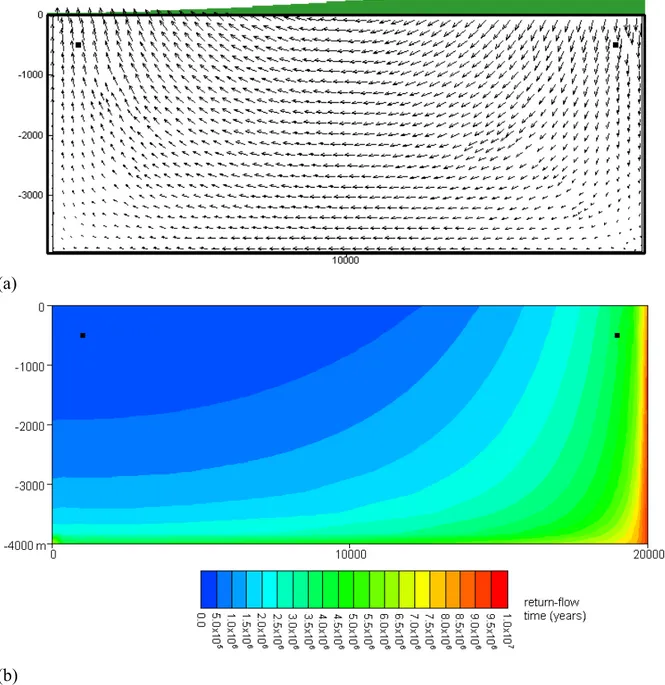
(a)
(b)
Figure 1. Simple case with no fracture zones: (a) sinusoidal water-table topography (green) and velocity vectors for the regional flow field; (b) map of return-flow times. Black squares denote hypothetical repositories at 500 m depth in the recharge (right) and discharge (left) areas. Vertical exaggeration is 2 times (2x). Elevations in (m).
Under the imposed head gradient, water enters the ground along the right side of the top boundary (the regional recharge area) and exits along the left side of the top boundary (the regional discharge area). For contaminants released from a hypothetical repository located 1 km from the right-hand boundary and 500 m below the top of the model (in the recharge area), the simulated
return-flow time is about 3.9 million years (Ma). This value agrees reasonably well with the value
of 3.4 Ma obtained by Toth & Sheng (1996) using a different method to compute ground-water age. For a repository sited in the discharge area (1 km in from the left-hand boundary and 500 m below the top of the model domain), the return-flow time is only 0.11 Ma.
Overall, for nearby locations in the region of the recharge-area repository at 500 m depth,
return-flow times are all approximately 5 Ma. For nearby locations in the region of the discharge-area
repository at 500 m depth, return-flow times all are approximately 0.1 Ma. Thus, repository locations in the recharge area have return-flow times about 50 times greater than repository locations in the discharge area, and path lengths about 40 times greater. All other factors considered, longer ground-water systems would have proportionally longer paths and return-flow
times. For example, in a 60-km-long system, the return-flow time would be about 150 times
greater and the path length 120 times greater than for the recharge-area repository than for the discharge-area repository. This relative time advantage could be even greater in variable-density fluid systems like the Fennoscandian shield, where deep saline flow systems have velocities thousands of times lower.
In the Fennoscandian shield, hydraulic conductivities for the rock matrix (considered unfractured at the kilometer scale) are similar to the case considered, whereas porosities are typically one to two orders of magnitude lower than those assumed in this example (Voss & Andersson, 1991). In this case, all else being equal, the return-flow times would be reduced by one to two orders of magnitude. If the rock matrix in Sweden were considered to include the kilometer-scale network of fractures zones assumed by Voss & Andersson (1991), the rock matrix would have one to two orders of magnitude higher conductivity, and return-flow times would be a total of two to four orders of magnitude shorter than in this example. Hydraulic gradients, which also affect return-flow times, may be higher or lower than in this example, depending on location. Ratios of travel
times and path lengths for the recharge- and discharge-area repositories would remain the same.
Return Flow Times with Local Topographic Variation and Conductive
Fracture Zones
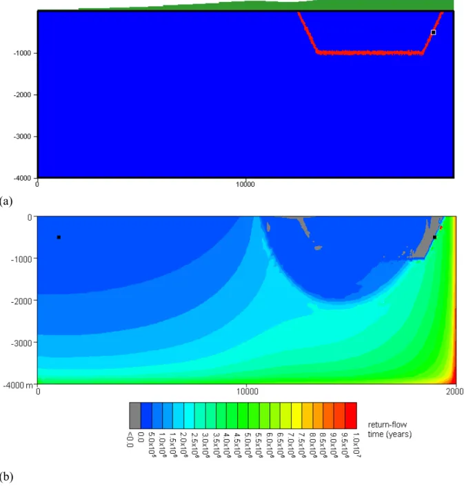
The presence of undulations in topography or highly conductive fracture zones may affect the location of primary recharge areas in ground-water systems. The distribution of return-flow times for the case in which a valley separates the recharge area from the regional discharge area are shown in Figure 2. Additionally, a nonlinear conductive fracture zone (or a series of connected fracture zone segments) passes through the repository and outcrops in the valley. The fracture zone is 100 times more permeable and 10 times more porous than the rock matrix. For this
water-table configuration, but in the absence of the fracture zone, an additional simulation (not shown) gives a return-flow time in the general vicinity of the recharge-area repository of 3.7 Ma, similar to that obtained in the case shown in Figure 1. The local valley causes a local ground-water system to develop above the deeper regional system. The local system is visible as the curved, darker blue area in the upper right portion of the model (Figure 2). The local system is present even without fracture zones. Water in the shallow system discharges near the local valley, shortening travel time and path length for repositories located within this shallow ground-water body. The upstream repository, when there is no fracture zone, is within the regional flow system. However, the fracture zone disturbs and offsets the upstream portion of the dividing line between the shallow and deep systems, whereas the downstream portion is not strongly affected. If the fracture zone is present, the shallow flow system captures discharge from the repository because the upstream boundary of the shallow system is shifted just beyond the repository location. With the fracture zone in place, the return-flow time decreases by approximately a factor of 10.
Overall, for most locations within the shallow local flow system (i.e., within the darker blue area) the return-flow time is on the order of 0.1 Ma or less, whereas for repositories situated in the recharge area of the regional flow system (to the right of the darker blue area), return-flow time is on the order of 5 Ma or greater. Repositories located within the local system have little advantage (in terms of return-flow time) over repositories located at 500 m depth within the regional discharge area, which also have return-flow times on the order of 0.1 Ma.
(a)
(b)
Figure 2. Variation on the base case – fracture zone and valley present: (a) surface topography
(green) and fracture zone (red); (b) map of return-flow time. Black squares denotes hypothetical
repositories in the recharge and discharge areas. Vertical exaggeration is 2x. Elevations in (m). Gray color indicates zones of numerical instability.
Return Flow Times that Illustrate Relations in Southeastern Sweden
Return-flow times within a two-dimensional (2D) vertical cross section of southeastern Sweden
that passes approximately through the repository sites considered later in the three-dimensional (3D) model is shown in Figure 3. This 2D result is shown only for illustrative purposes as it entails major simplifications in comparison with the 3D model described later, and it represents only one possible model of the bedrock properties. Because of these simplifications, the
return-flow time distribution shown here only should be considered as indicative of its spatial
distribution; furthermore, absolute values may be quite different from the 3D model with the same bedrock properties.
The hydrogeologic properties represented by this 2D model are those of the 10:1 Case (10:1 horizontal-to-vertical anisotropy in the permeability) described later in reference to the 3D model (see the section titled “Representation of the bedrock fabric”). Here, only constant-density fluid flow is considered. Further, the model reaches a depth of only 3 km, although the 3D model described later reaches 10 km depth. The bottom of the 2D model may be considered as being approximately at the depth of shield brines, which act approximately as a no-flow boundary to the freshwater flows above. The topography along the top of this 2D model is exactly that of the 3D model (see Figure 4) along the line of section shown in Figure 3. The repository locations are at a depth of 500 m.
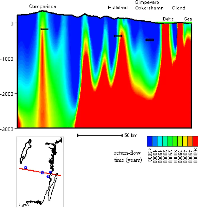
The map of return-flow times clearly illustrates how the undulating topography of southeastern Sweden may generate both regional and nested local flow systems. Repository locations within the red band have very long return-flow times, whereas repository locations within the blue band have relatively very short return-flow times. Note that zones of red (the highest return-flow
times) always should reach up the land surface, as the longest times would occur at locations on
the surface in recharge areas. However, because there is a finite amount of dispersion in the numerical model, they do not occur at these locations, and so the results require some interpretation in terms of what an ideal model without dispersion would give.
The primary regional system described in this section has recharge below the topographic peak near the left margin of the top boundary and discharges both to the left boundary (near Vättern Lake) and to the Baltic Sea (top right boundary). Repository locations within the regional system have the longest return-flow times in the section. The ‘Comparison site’ is located below the
Figure 3. Cross-section through repository sites (black boxes) showing return flow times for illustrative simulation (10:1 Case). Baltic Sea level is shown as green region along top right boundary. Inset shows section location (red line) and repository sites (in blue) and refers to the map in Figure 4. Repository sites – left to right, in cross section – are ‘Comparison’, Hultsfred, and Simpevarp/Oskarshamn. Vertical exaggeration is 40x. Elevation on left edge of cross section is given in m.
Evaluation of Southeastern Sweden Repository Sites
REGIONAL HYDROGEOLOGY
The hydrogeology of southeastern Sweden is considered on a regional scale. This is necessary to allow consideration of regional-scale ground-water flow systems that may exist in the region, which in turn allows identification of recharge areas for the regional flow systems. Flow is
considered to be driven by a combination of regional as well as local hydraulic gradients, whereas hydraulic properties can practically only be considered as regional averages because of the local complexity of the conductive fabric of the bedrock.
Study area
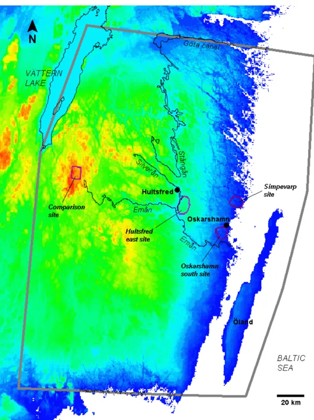
This study focuses on the portion of southern Sweden to the east and south of Vättern Lake, with special attention paid to the vicinity of three proposed repository sites: Hultsfred east, Simpevarp, and Oskarshamn south (SKB, 2001). The study area and model domain are shown in Figure 4. The model domain extends beyond the immediate vicinity of these sites to allow the setting of natural hydrologic boundary conditions, to allow the model to naturally generate regional flow systems, and to provide a basis for comparing the proposed sites with alternative sites in southern Sweden.
The land-surface elevation of the study area also is shown in Figure 4. Elevation data were obtained from LMV (Lantmäteriverket, 2000) on a grid of 500 m. Normally, in humid regions, the water-table elevation generally follows at some small depth below the land-surface elevation. Therefore, for the purposes of driving ground-water flow in this modeling study, the land-surface elevation is used as an approximation of the water table.
Bedrock hydrogeology
is indirect at best. The present study addresses the uncertainty in regional connectivity of permeable structures by considering the effect of varying degrees of horizontal and vertical fracture connectivity on the regional hydraulic conductivity of the bedrock. The depth dependence of hydraulic conductivity in the shield rock also is highly uncertain. Hydraulic conductivity appears to decrease below a depth of 200 m; measurements to date show no other trend to a depth of about 1 km (Winberg, 1989), and few measurements are present below this depth. A variety of indirect evidence, including information from the Kola super-deep borehole in northwest Russia and widespread seismic low-velocity zones in the Fennoscandian shield and elsewhere, suggest that much of the rock permeability disappears by a depth of 8 to 10 km (Neuzil, 1995). Permeability may decrease due to high temperatures, diagenesis, and prevention of fracture formation or closing of fractures by high lithostatic load.
To the east and southeast of Oskarshamn, crystalline rock is overlain by sedimentary layers extending below the Baltic Sea to central Europe (Kornfält & Larsson, 1987; Ahlbom and others, 1990; Grigelis, 1991). Near Sweden, the sedimentary overburden consists of the following sequence: Lower Cambrian sandstone, Middle Cambrian claystone/shale, Upper Cambrian alum shale, Ordovician limestone, Silurian chalk/marl, and Devonian chalk/marl. Relative to the surrounding rock, the sandstone is highly conductive, whereas the shales form an aquitard that extends (at least) 200 km to the east of Oskarshamn (Kornfält & Larsson, 1987).
Flow field and distribution of fluids
The Fennoscandian shield is assumed here to be hydraulically conductive to a depth of about 10 km. Under present-day climatic conditions, subsurface water moves from recharge areas at higher elevations to discharge areas at lower elevations. The coast of Sweden apparently serves as a discharge area for many recharge areas in the regional flow system, whereas at higher elevations inland, smaller-scale recharge-discharge systems occur.
Four types of ground water are generally found in the Fennoscandian shield: recent recharge water of low total dissolved solids (TDS) content, relict glacial meltwater with low TDS, relict seawater at concentrations up to one-third (about 10000 mg/LTDS) of today's ocean water, and shield brine (Glynn & Voss, 1996). The freshwater generally is found at shallow depths at all locations and may be found at greater depths with increasing distance inland from the coast. The regional spatial distribution of the relict glacial meltwater is poorly known; it is found at varying depths at most sites investigated, and likely originates from sub-glacial meltwater of the last glaciation. The relict seawater generally is found in Sweden at locations with surface elevation below about 200 m, and may stem from the period of marine incursion following the last glaciation about 10 ka before present (BP) (Lindewald, 1981, 1985).
Shield brine generally may be found at any location below the fluids described above. Near the coast and other major discharge areas, shield brine is found near the surface, whereas further inland it usually is found at greater depths. Nordstrom and others (1989a) have summarized the various mechanisms that have been proposed for brine formation in crystalline rocks. Both allochthonous (external to the rock) and autochthonous (internal to the rock; arising from rock-water interaction) sources of salinity have been proposed. Mechanisms based on rock-rock-water interaction include silicate mineral hydrolysis (Edmunds and others, 1984) and leakage from saline fluid inclusions (Nordstrom and others, 1989b).
Because of the large density contrast between freshwater and shield brine, circulation of shield brine likely is driven by both fluid density differences and topographic gradients, whereas flow of the more dilute fluids, including relict seawater, is driven primarily by topographic gradients (Voss and Andersson, 1993).
The complex pattern of fracture zones and permeable structures in the shield suggests that the three-dimensional spatial distribution of fluid types may be complex. Therefore, these distributions and the flow field are difficult to interpret in detail for any particular area, even on the basis of intensive hydrogeologic field programs. Any detailed description of the spatial distributions of permeable structures and fluids is certain to be incomplete, at best, and the evolution of these distributions through time is subject to even more uncertainty. Most often, only broad generalizations of the kind made in this study can be advanced with any confidence.
DESCRIPTION OF THE 3D MODEL
Extent and discretization of the 3D model
The model covers a roughly rectangular area that includes the portion of Sweden to the east and south of Vättern Lake. The model domain extends approximately 260 km north to south and 210 km east to west, covering an area of approximately 49,000 km2 (Figure 4). Vertically, the model extends from the land surface (with a variable elevation given by the digital elevation grid) to a depth of 10 km below sea level. The model U.S. Geological Survey’s SUTRA code was used in three spatial dimensions (Voss and Provost, 2001, personal communication). Input data for the 3D model were generated using a 3D version (Winston and Voss, 2001, personal communication) of SutraGUI (Voss and others, 1997), a graphical interface for the SUTRA code.
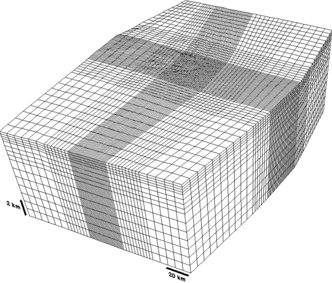
The finite-element mesh of the region in plan view is shown in Figure 5. An oblique view of the three-dimensional mesh exaggerated ten times in the vertical direction is shown in Figure 6. The finest discretization is in the vicinity of the Hultsfred site, near the land surface, where the elements measure approximately 1,500 m on a side horizontally and 250 m vertically. The coarsest discretization is in the southwestern portion of the model, near the bottom, where the elements measure roughly 10,000 m on a side horizontally and 1,000 m vertically. The distribution of elements was designed to provide finer discretization in the shallow subsurface in the vicinity of the sites and in the network of stream valleys that runs among the sites (including portions of the streams, Strångån, Silverån, and Emån, see Figure 4), which was expected to strongly affect the flow field. The mesh has 15 elements vertically, 58 east-west, and 64 north-south, totaling 55680 elements and 61360 nodes. This mesh must be considered as a rather coarse discretization of the region; however, present limits on convenient computing resources preclude
The LMV data give lake water levels, not bathymetries. Equating the surface of the model with lake water levels is considered unlikely to cause substantial error, given the relatively small area and shallow depth of the lakes in the region compared with the model domain. The exception is Vättern Lake, which is relatively large and deep. Beneath Vättern Lake and the Baltic Sea, the surface of the model is based on bathymetric data (Tirén, S., 2000, personal communication), which were represented as contours in the graphical user interface and transferred to the meshed data layer along with the land surface elevations.
Figure 6. Oblique view (from southeast towards northwest) of three-dimensional finite-element mesh. (Vertical exaggeration = 10x)
Representation of the bedrock fabric
Crystalline bedrock is treated here as a continuum with an effective hydraulic conductivity that accounts for the presence of the regional network of fracture zones. The conductivity may be anisotropic (different values for different flow directions) or isotropic (same values for all flow directions). Individual fracture zones are not resolved at the regional scale of this model; indeed, a three-dimensional map of fracture zones is not available for the region and would be impossible to create with any certainty. Hydraulic conductivity and anisotropy of hydraulic conductivity must be considered on a large scale for purposes of modeling.
The sedimentary units along the southeast coast are not included in the present model, and the region where these layers are present is assigned properties of granodiorites equivalent to the rest of the model. It may be expected that the presence of the sediments as a confining unit would tend to force discharge from the terrestrial flow system closer to the east coast of Sweden than in the case where they are neglected, shortening travel times and flow paths for near-coastal repository locations. Thus, neglecting the confining units in this analysis is an optimistic approximation for near-coastal repository locations because it lengthens travel times and flow paths for these locations.
Decreases in conductivity with depth could be represented in the model by a layered conductivity profile; however, these are not considered, and all simulations assume constant conductivity with depth. The subsurface fluid density increases with depth in the simulations, and fluid flows are substantially lower in the denser fluids. Thus, the presence of high density at depth in the model gives an effect on the shallower flow field and on the decrease in fluid flux with depth similar to that of a decreasing conductivity with depth. Decreasing the conductivity at depth would most likely have the greatest effect on long, deep flow paths. Some of these flow paths could be displaced into shallower, more conductive layers, thereby decreasing their return-flow times, whereas the return-flow times for flow paths that remained in deeper, less conductive layers would likely increase. Given the considerable uncertainty in the variation of conductivity with depth and in the spatial distribution of fluid density, it was decided not to include depth-dependent conductivity in the present analysis.
Hydraulic permeability and porosity in the crystalline basement are based on the ranges of values given by Voss & Andersson (1991, 1993) for various assumptions based on Sweden’s bedrock, about fracture zone spacing and direction (e.g. spacing of horizontal zones on the order of
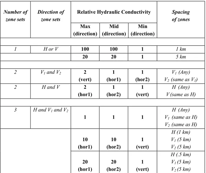
Simple calculations for equivalent porous media representations of fractured rock (using in-series and in-parallel models of fracture zones and the host rock) show that the bedrock, on a regional scale, may not be extremely anisotropic (Table 1). If the rock contains only a single set of parallel conductive fracture zones (with the conductivities described above) then the maximum possible anisotropy in hydraulic conductivity is less than 100:1 (maximum permeability : minimum
permeability) for spacing of about 1 km and about 20:1 for 5 km spacing, with the higher
conductivity value in the directions parallel to the fracture zones. For a case with two nearly perpendicular sets of equally spaced parallel fracture zones (each with the same properties and spacing), the maximum possible anisotropy in hydraulic conductivity is only 2:1, with the higher value oriented along the direction of intersections of the two sets of fracture zones. For three equally spaced mutually perpendicular sets of parallel fracture zones, the bedrock conductivity tends to be approximately isotropic (e.g., 1:1 or 10:10). If spacing of one set of the three were different from the others, then anisotropy could be higher; for example, 10:1 or 20:1 for typical spacings.
For the bedrock within the model area of southeastern Sweden, it may be speculated that it is unlikely that there is only one set of conductive fracture zones. If there are two conductive mutually perpendicular fracture zone sets throughout, then the regional scale anisotropy is on the order of 2:1. If the two sets are aligned horizontally and vertically, then horizontal conductivity along the direction of the zone intersections is about two times higher than in the other directions. If the two sets are both aligned vertically, then the vertical conductivity is about two times higher than in the horizontal directions. If there are three mutually perpendicular fracture zone sets throughout the bedrock, then anisotropy may range from isotropic for equal spacing and properties (e.g., 1:1 or 10:10) to about 10:1 or 20:1 for unequal spacing or properties, probably with the horizontal conductivity higher than the vertical conductivity. Thus, the full range of anisotropy in effective hydraulic conductivity that is possible in the bedrock is between about 2 times higher vertically than horizontally to 20 times greater horizontally than vertically. This range includes the possibility of isotropic bedrock.
For the numerical modeling, four cases are considered with respect to distribution of fracture zones in the bedrock. These cases are chosen to represent the full range of possible average anisotropies of the bedrock. In this study, areal anisotropy is not considered, and the bedrock is allowed only horizontal-vertical anisotropy. In the case with only vertical zones, local topographic gradients would have their greatest effect on the system, resulting in deeply penetrating local flow cells. This case would result in the shortest flow paths from a repository and the poorest performance of an upstream repository. To exaggerate this pessimistic case for recharge-area repositories, although the greatest possible vertical anisotropy is only 1:2, a case is considered here with anisotropy of 1:10, where the vertical conductivity is 10 times higher than horizontal conductivities. The situation that would result in the largest regional flow systems is the one with the highest horizontal anisotropy, or 20:1, where vertical conductivity is less than horizontal conductivity. To reduce the advantage of this situation for recharge area repositories, only a case of 10:1 is considered.
The four cases selected to represent the possible range regional anisotropy in hydraulic conductivity of the bedrock are given below.
10:1
Average horizontal hydraulic conductivity of the bedrock is 1.0x10⁻⁸ m/s and average vertical conductivity is 10 times less, 1.0x10⁻⁹ m/s. These values derive from an equivalent porous
medium representation of bedrock with two perpendicular sets of sub-vertical fracture zones and a set of sub-horizontal fracture zones (Voss & Andersson, 1991, 1993). Zones are about 50 m wide, with a vertical spacing of about 1 km and a horizontal spacing of 5 km. Similarly, these average values represent a family of bedrock configurations that includes, for example, one with 25 m wide zones with vertical spacing of 0.5 km and horizontal spacing of 2.5 km. The rock has anisotropic conductivity with horizontal conductivities 10 times greater than vertical conductivity, or ‘10:1’ anisotropy.
10:10
This case represents bedrock that consists of three mutually perpendicular sets of parallel fracture zones (e.g., one sub-horizontal set and two vertical sets) with approximately the same spacing in each direction. There is about one 5-m wide conductive zone per km in all directions. The resulting average bedrock conductivity is approximately isotropic with conductivities of 1.0x10⁻⁸ m/s.
1:1
The 1:1 case represents the same situation as the 10:10 case, but where overall conductivities are 10 times lower (1.0x10⁻⁹ m/s). This case is equivalent to fewer conductive zones per km and/or
lower zone widths.
1:10
This case represents the bedrock where there is an extremely high vertical conductivity in comparison with the horizontal conductivity. The case derives from an equivalent porous medium representation with two perpendicular sets of conductive sub-vertical fracture zones and without well-connected conductive sub-horizontal fracture zones. Average vertical hydraulic conductivity of the bedrock is 1.0x10⁻⁸ m/s and average horizontal conductivity is 10 times less, 1.0x10⁻⁹ m/s. The 1:10 case would represent an extreme vertical anisotropy for bedrock with two or more intersecting sub-parallel fracture sets as described above. However, it is considered here to establish return-flow time results for a bounding situation in the bedrock where local topographic gradients potentially are more important than semi-regional or regional gradients in establishing
Relative Hydraulic Conductivity Number of zone sets Direction of zone sets Max (direction) Mid (direction) Min (direction) Spacing of zones 1 H or V 100 100 1 1 km 20 20 1 5 km 2 V1 and V2 2 (vert) 1 (hor1) 1 (hor2) V1 (Any) V2 (same as V1) 2 H and V 2 (hor1) 1 (hor2) 1 (vert) H (Any) V(same as H) 3 H and V1 and V2 1 1 1 H (Any) V1 (same as H) V2 (same as H) 10 (hor1) 10 (hor2) 1 (vert) H (1 km) V1 (5 km) V2 (5 km) 20 (hor1) 20 (hor2) 1 (vert) H (.5 km) V1 (5 km) V2 (5 km)
Table 1. Regional effective anisotropy of bedrock containing sets of conductive fracture zones. Principal hydraulic conductivity values in maximum (Max), middle (Mid) and minimum (Min) directions of anisotropic hydraulic conductivity are given relative to the minimum value.
Depending on the configuration of zones, these values may be oriented in the vertical direction (vert), or in one of the mutually perpendicular horizontal directions (hor1 or hor2). Each set is assumed to occur as sub-parallel zones oriented either horizontally (H) or vertically (V, V1 and
V2). Zone widths are assumed to be much less than the spacing between zones. Two or more sets
of zones occurring simultaneously are assumed to be mutually perpendicular. Each zone is 50-m wide with hydraulic conductivity of 2.x10-7 (m/s) and the remaining bedrock has hydraulic
conductivity of 1.x10-10 (m/s). Spacing of zones in each set is given in the table. Spacings are equal when referring to more than one set. These anisotropies proportionally also represent other zone spacings, widths, and hydraulic conductivity.
Modeling of physical processes and boundary conditions
The U.S. Geological Survey computer code SUTRA (Voss, 1984, two-dimensional code) was upgraded for three-dimensional simulation (Voss and Provost, 2001, personal communication) and used to model variable-density fluid flow in southeastern Sweden. Variable fluid density is required for model simulation because of the presence of shield brines at depth in the bedrock with significantly higher density than the freshwater found in shallower regions. For each bedrock permeability case considered, a steady-state flow and solute concentration was simulated to represent present-day conditions. Repository siting then was evaluated on the basis of this flow field. It is not known whether the present ground-water system has reached a steady state following the substantial glacial-climatic stresses experienced over the past 20 Ka. However, Provost and others (1998) have shown that in the amount of time elapsed in the present interglacial, it is possible to nearly reach a steady state.
The model considers the formation of shield brine as a process that depends on the difference between concentration of dissolved solids in the ground water and the potential dissolved solids concentration contributed by rock weathering, leaching of saline fluid inclusions, or other processes (Nordstrom and others, 1989a). The rate of brine formation is represented (Provost and others, 1998) by a first-order expression, rate = kmt(Cmax – C), where C is the concentration of
total dissolved solids in the ground water, Cmax is the maximum allowable concentration of dissolved solids, and kmt is a rate constant (or mass transfer coefficient) for rock-water mass
transfer. In the case of rock weathering, Cmax could represent the saturation concentration of dissolved solids (treated as a single species), whereas in the case of leaching of inclusions, it could represent the concentration of dissolved solids in the inclusions.
The simple expression, defined above, for the rate of brine formation captures two essential features of the rock-water interaction: the rate at which solids dissolve in the pore fluid decreases as their concentration in the fluid increases and dissolution ceases when the concentration reaches the maximum allowable value. Despite its simplicity, this expression can be adjusted to approximate the general present-day trend in the concentration profile of dissolved solids observed in the field, and its incorporation into the model allows the density distribution to evolve along with the pressure field in a "natural" and consistent way. The expression does not depend on what particular geochemical process actually generates the shield brines, as it accommodates a number of possible origins. The value of the mass transfer coefficient, kmt, was not known a
In each case of bedrock hydraulic conductivity considered, kmt was chosen such that a
concentration of 0.1(Cmax) was located at a maximum depth of 3 to 5 km beneath the southern Swedish highlands. This approach provided an approximate correspondence with the 2D results of Provost and others (1998), which in turn were approximately calibrated to concentrations measured in two boreholes, one within the region of the present model. Thus, for each case, the model was adjusted such that the modeled concentration field approximately matched the available salt-distribution data.
A no-flux condition is imposed at the bottom boundary of the model to represent the depth at which the bedrock permeability is so small (because of lithostatic loading and high temperatures) that it can be considered zero for this model. The western boundary is assumed to be approximately a ground-water divide, and a no-flux condition is imposed there. The northern boundary is assumed to be approximately along a streamline, and a no-flux condition is imposed there. The southern boundary is a no-flux boundary that approximately follows the coastline, under the assumption that most southward ground-water flow will discharge upward upon reaching the Baltic Sea. Likewise, the offshore boundary to the east is assumed to be a no-flux boundary. Both the southern and eastern boundaries are assumed to be sufficiently far removed from the area of interest that the model-simulated terrestrial flows would not be affected by the choice of hydrostatic pressure or no-flux as boundary conditions at these locations.
On land, the top boundary of the model is set to a specified pressure of zero (i.e., atmospheric pressure), and any inflow that occurs along the top boundary is assigned a salt concentration of zero (freshwater) for the steady-state flow-field simulation. The elevation of the top surface of the model is intended to represent the water table on the land portion, and is set to the value given by the elevation grid. Beneath Vättern Lake and the Baltic Sea, the top of the model follows the bathymetry, and pressure is set as the hydrostatic value according to the depth and density of each type of water. Vättern Lake elevation is set to 89 m (Tirén, S., 2000, personal communication). The concentration assigned for lake water is zero; the concentration assigned for Baltic Sea water is 0.005 kg-solute/kg-fluid (about 1/7 standard seawater).
Dispersion coefficients for transport of salt are set to relatively low values, considering the coarse discretization used in the model. The values are chosen arbitrarily, as no data are available for transport in the Fennoscandian shield at the scales of transport considered in this model domain. However, the values are not unreasonable for the scale of solute transport in the system under consideration.
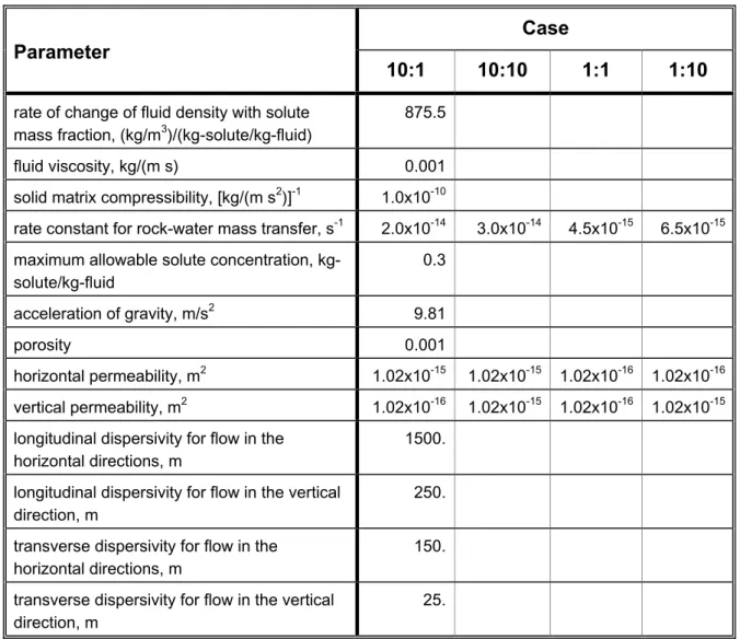
Model input data
Case Parameter
10:1 10:10 1:1 1:10
rate of change of fluid density with solute mass fraction, (kg/m3)/(kg-solute/kg-fluid)
875.5 fluid viscosity, kg/(m s) 0.001 solid matrix compressibility, [kg/(m s2)]-1 1.0x10⁻¹⁰
rate constant for rock-water mass transfer, s-1 2.0x10⁻¹⁴ 3.0x10⁻¹⁴ 4.5x10⁻¹⁵ 6.5x10⁻¹⁵
maximum allowable solute concentration, kg-solute/kg-fluid 0.3 acceleration of gravity, m/s2 9.81 porosity 0.001 horizontal permeability, m2 1.02x10⁻¹⁵ 1.02x10⁻¹⁵ 1.02x10⁻¹⁶ 1.02x10⁻¹⁶ vertical permeability, m2 1.02x10⁻¹⁶ 1.02x10⁻¹⁵ 1.02x10⁻¹⁶ 1.02x10⁻¹⁵ longitudinal dispersivity for flow in the
horizontal directions, m
1500. longitudinal dispersivity for flow in the vertical
direction, m
250. transverse dispersivity for flow in the
horizontal directions, m
150. transverse dispersivity for flow in the vertical
direction, m
25.
Table 2. Input parameters for four models of variable-density ground-water flow and brine transport in southeastern Sweden, corresponding to four cases representing properties of the bedrock. Entries not shown are the same as for the 10:1 Case.
RESULTS OF 3D MODELING
The flow field is evaluated and path lengths and travel times from each of four repository locations in southeastern Sweden are determined for the four cases of the bedrock permeability.
Steady-state flow fields and salt distributions
A 3D view of the complete model domain shows the steady-state salt distribution for the bedrock 10:1 Case (horizontal permeability: vertical permeability = 10:1) (Figure 7). Shading indicates the relief on the top surface of the model. Dark blue indicates the fresher water and generally covers the land surface; recharge to Öland is visible in the dark blue stripe offshore.
The internal steady-state salt distribution for each bedrock case along a vertical section that runs approximately east to west through the Simpevarp site is shown in Figure 8. Because the permeability distribution was different for each case, the mass transfer coefficient, kmt, was
adjusted, in each case, by trial-and-error in a sequence of simulations until a near-steady salt distribution was achieved that matches available field data. These field data were used for a similar purpose by Provost and others (1998). (Simulations were performed using the ORTHOMIN iterative solver for pressure and concentration.)
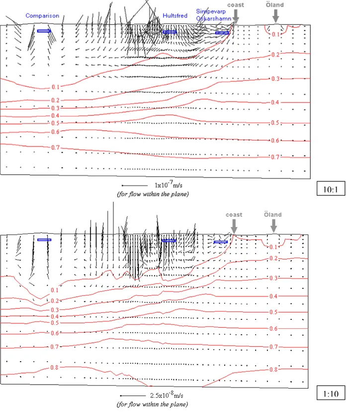
A close view of the vertical cross section for the 10:1 Case in Figure 9 highlights the variable-density flow field. This section is similar to that shown in Figure 3, and the return flow times shown in Figure 3 may be approximately compared with the velocities shown in the upper part of
Figure 9 (10:1 Case). (A map of return flow times based on the 3D model along the section in Figure 9 could be generated based on the same procedure used to generate the return flow time
maps at 500 m depth. These maps are shown and discussed later in this report. It was deemed unnecessary to show these for the purpose of the present illustration.) Note that the areas of downflow near the surface in Figure 9 (10:1 Case) are in regions where the return flow times are very high near the surface in Figure 3. These are the areas of recharge to the deeper ground-water-flow systems. Recharge is at relatively higher elevations, and discharge is at relatively lower elevations of the top surface. The flow field is complex as a result of rotational flow due to variable density and because of the undulating surface topography. A distinctive feature is the zone of discharging fluids near the coast. Note also that flow velocities at depth are very low; these low velocities are a result of the dense fluids at depth, which retard the deep penetration of the fresher, more buoyant water that is recharged at the surface.
Ideally, a repository could be placed in a recharge area for the deep flow systems to maximize
return flow times. For the 10:1 Case, the Comparison site and eastern portion of the Hultsfred-east site are in broad-deep regions of downflow, whereas the coastal Simpevarp and Oskarshamn-south sites clearly are located within the coastal discharge area. For the 1:10 Case
(lower part of Figure 9) the vertical components of flow are much greater (relative to horizontal) than in the former case. In this case, however, the Comparison site is still in a broad, deep region of downflow. Also, much of the Hultsfred-east site is still in a broad, deep region of downflow, though there may be a small upflow near the easternmost margin of the site. The Simpevarp and
Oskarshamn-south sites are still clearly located within the coastal discharge area, though there
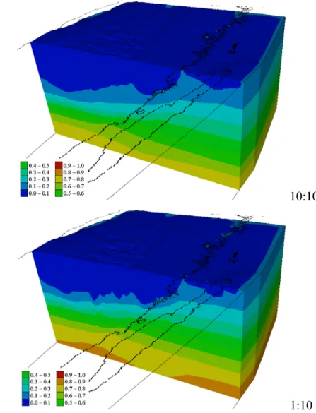
10:1 10:10
1:1 1:10
Figure 8. Salt distributions for four bedrock cases (horizontal permeability : vertical permeability). View from southeast. East-west section approximately through Simpevarp. Vertical exaggeration = 10x. Concentrations shown are fractions of maximum salt concentration.
Figure 9. Salt concentration and flow field for bedrock Cases (10:1) and (1:10). Cross-section viewed from the south. (Similar, though not identical, section as in oblique view of Figure 8.) Vertical
10:1
Flow paths
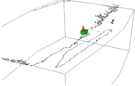
Flow paths for each repository site are shown as colored 3D flow tubes for the two bounding bedrock
cases, 10:1 and 1:10, in Figure 10 and in Figure 11. These two cases should provide the longest (for 10:1) and shortest (for 1:10) possible paths among the bedrock models considered here. The length of the flow path from each repository in each of these two cases may be estimated from the model result. These lengths are summarized in Table 3.
Each simulation results in a flow tube traced in 3D from the repository location to the point(s) of exit from the model domain. A flow tube may exit at one location or it may split and exit at a number of locations. The flow tube represents a plume of conservative solute emanating from the entire repository site. Ideally, flow tubes in 3D should be traced in a model with no dispersion. As this is not possible in these model simulations, flow tubes must be traced using solute transport with dispersion and by tracking concentration.
The flow tube approximately traces out the subsurface region into which any escaping radionuclides from a repository would potentially spread. In these simulations, dispersion was kept near the minimum required to maintain numerical stability. Higher dispersion in the model tends to widen the flow tubes, possibly causing solute to enter adjoining flow paths that do not pass through the repository, and thus would tend to exaggerate the flow-tube volumes. Flow tubes are visualized by selecting the lowest value of concentration whose isosurface exhibits a minimum of branching and also connects the repository with discharge points. Sometimes, it is not possible to track a low concentration from the site to its ultimate discharge point because the flow path is obscured by the dispersion required to maintain numerical stability in the coarse mesh. In this situation, the path length in Table 3 is indicated as being greater than the path length that could be tracked. The volumes of the flow tubes, as visualized in the present model, must be considered as approximate indicators of the actual path volumes, and should be used for relative comparison among the sites; this is both because dispersion is not zero and because an arbitrary concentration level is selected for tube display.
Flow paths are simulated by selecting a set of nodes in the mesh at a depth of 500 m in the designated
repository area at which concentration is specified as an arbitrary non-zero value. The concentration of recharge from the top surface is set to zero. A single transport solution for a very long time step (e.g., 1013 years) is obtained (with the GMRES solver) to approximate steady transport conditions given the flow field from the steady-state variable density simulation for each case.
To facilitate tracking of advective tracer transport, an effort was made to use the minimum amount of dispersion possible while maintaining numerical stability. For the 10:1 case, the longitudinal dispersivities are set to ¼ of the representative mesh spacing in the direction of flow: for horizontal flow, they range from 450 m in the central portion of the mesh to 2500 m in the outer portion; for vertical flow, they range from 62.5 m near the top surface to 500 m near the bottom of the model. For the 1:10 case, the longitudinal dispersivities are set 3 times as high as for the 10:1 case. In both cases, the transverse dispersivities are set to 10 m throughout the model.
It may be seen that, in the 10:1 Case, the flow paths from the Simpevarp and Oskarshamn-south repository sites near the coast are very short, nearly vertical and tending upwards towards the coast (Figure 10). Path lengths from these sites are about 3 km or less. (Because of the large size of the finite elements in the area, path lengths shorter than 3 km, which may be possible in these locations, cannot be resolved.) These path lengths are about an order of magnitude shorter than the longest paths from Hultsfred-east, where flow occurs from west to east (left to right in Figure 10) over a distance of about 25 km before discharging at an inland point and a distance of about 50 km before discharging at the coast. The comparison site, situated in a highland area in the western portion of the region, has the longest flow path that discharges at the east coast. The path length is about 130 km. Another flow tube from the site discharges at Vättern Lake, a distance of about 60 km. At both Hultsfred-east and the
comparison site, the path begins in a direction directly downward from the repository location for a
few km before becoming horizontal.
In the 1:10 Case, the flow paths from the Simpevarp and Oskarshamn-south repositories near the coast are again very short, about 3 km or less (Figure 11). At the Hultsfred-east site, the flow tube leaves the repository directly downwards until at a few kilometers depth, it turns upwards towards the coast and then becomes difficult to track further in the model. The path length is at least 30 km, as far as the tube can be tracked in the simulation. There also are some local upflows from some locations within the site with very short path lengths. At the comparison site, the flow tube leaves the repository directly downwards until at several kilometers depth, it splits into two parts. One tube travels to the east, but concentrations in the simulation are too low to track the plume to its discharge point, possibly at the coast (path length at least 45 km long). The other tube rises towards a discharge point south of Vättern Lake along the model boundary (path length about 35 km long). At the margins of this site there are locations that have local upflows with very short path lengths.
Notwithstanding the approximations inherent in visualizing flow tubes discussed above, for both extreme bedrock cases considered here, the volumes of the plumes and, thus, the flow path volumes are much greater for the Hultsfred-east and comparison sites than for the coastal sites. This result also is an obvious consequence of the greater path lengths for the inland sites where flow path volume ratios between long and short flow paths would tend to be at least as great as the ratios of the path
Simpevarp site. Shows C/Csource>0.50. Oskarshamn-south site. Shows C/Csource>0.20.
Hultsfred-east site. Shows C/Csource>0.13. Comparison site. Shows C/Csource>0.29. (Plume to the north shown in blue for
clarity.)
Travel time (ka) Path length (km) Repository Site Case (10:1) Case (10:10) Case (1:1) Case (1:10) Case (10:1) Case (1:10) Simpevarp 1 →10 1 →10 10 →100 10 → >100 < 3 < 3 Oskarshamn-south 1 →10 1 →10 10 →100 10 → 100 < 3 < 3 Hultsfred-east (eastern part) 10 →100 1 →100 10 → >100 10 → 100 25, 50 >30 non-uniform Comparison 10 → >100 10 →100 10 → >100 10 → >100 60, 130 35, >45 non-uniform
Table 3. Approximate path lengths and travel times for all repository locations and bedrock cases. ‘Non-uniform’ indicates that there may be localized upflow within the repository site
Return-flow times
Maps of return-flow times at a repository depth of 500 m for each bedrock case are shown in
Figure 12. The return-flow time is the time required for fluid beginning at any point in the 3D
model domain to travel to its exit point from the domain. Thus, these maps show where, at 500 m depth, repository locations would have very high and very low travel times for escaping radionuclides. The return-flow times from each repository site in each of the four bedrock cases are summarized in Table 3. The general range of return-flow times for each site given in Table 3 is representative of only relatively large areas within each site, and small regions of higher or lower return-flow time are ignored. The details of distributions at each site may not be over-interpreted because the numerical mesh is relatively coarse; rather, the larger patterns of
return-flow times are most meaningful in these simulations.
The absolute level of return-flow times is directly proportional to the selected porosity value, but relations among return-flow times for the various cases considered are independent of the porosity. Thus, all return-flow times primarily should be considered in a sense relative to one another, as the individual values depend on the single bedrock porosity value selected for the simulations.
The return-flow time is calculated for approximate steady-state transport conditions. Because of difficulties with numerical stability for the relatively coarse mesh used when calculating a single-step steady state concentration solution (i.e., the usual technique used when the mesh is sufficiently fine), a stepwise approach was used to generate return-flow time maps at repository depth. Four special aspects of this type of simulation are listed below.
1- All flow is reversed in the simulation by negating the specified pressure boundary values, the gravity components, and the initial pressures (which result from the steady-state variable-density simulation). Any specified fluid sources and sinks also would have to be negated, but there were none in these simulations.
2- A zero-order solute source within the fluid is specified at a rate of one per year.
3- The SUTRA code was modified such that a concentration of zero is specified at surface nodes at which recharge occurs in the reversed flow. This corresponds to setting the return
flow time to zero at discharge points in the forward flow. This helped to mitigate the
effects of dispersion near the top surface of the model.