VTI notat 15A-2012 Published 2012
www.vti.se/publications
Coastdown measurement with 60-tonne tr
uck
and trailer
Estimation of transmission, rolling and air resistance
Ulf HammarströmRune Karlsson Harry Sörensen Mohammad-Reza Yahya
Preface
On commission of IVL AB, VTI has made a study of driving resistance parameters for a 60-ton truck with trailer. The contact person at IVL AB was Åke Sjödin. This project is included in an implementation program for HBEFA model financed by the Swedish Transport Administration. The contact person at the Swedish Transport Administration was Håkan Johansson. Ulf Hammarström, VTI, has been project leader.
The English translation of this document was controlled by Tarja Magnusson, VTI. We also would like to thank Alltransport AB, and especially Håkan Forsbäck, the truck driver, for good support. Finally we are most grateful to Martin Rexeis at Graz University of Technology for the scientific control of this document.
Quality review
Peer review was performed on 6 February 2012 by Martin Rexeis at Graz University of Technology. Ulf Hammarström has made alterations to the final manuscript of the report. The research director Maud Göthe-Lundgren, VTI, examined and approved the report for publication on 22 March 2012.
Kvalitetsgranskning
Peer review har genomförts 6 februari 2012 av Martin Rexeis at Graz University of Technology. Ulf Hammarström har genomfört justeringar av slutligt rapportmanus. Projektledarens närmaste chef, Maud Göthe-Lundgren, VTI, har därefter granskat och godkänt publikationen för publicering 22 mars 2012.
Innehållsförteckning
Summary ... 5
Sammanfattning ... 7
1 Background ... 9
2 Objective ... 11
3 A model for driving resistance ... 12
4 Problem description ... 18
5 Method ... 23
5.1 Introduction ... 23
5.2 The test vehicle ... 23
5.3 Measurement equipment ... 28
5.4 The test route ... 31
5.5 Measurement procedure for coastdown ... 32
5.6 Meteorological conditions ... 33
5.7 Measured data ... 33
5.8 Examples of driving resistance parameter values from the literature ... 38
5.9 Analysis ... 45
6 Results of measurements ... 49
6.1 Truck with trailer ... 49
6.2 Rigid truck ... 57
6.3 Discussion of measuring results ... 60
7 Comparison of measuring results with PHEM data ... 65
7.2 PHEM parameter values ... 65
7.2 Comparison of PHEM parameters with the coastdown study and with the literature ... 65
7.3 Discussion about PHEM parameters compared to the literature and the coastdown study ... 71
Discussion on a total level ... 73
Conclusions ... 75
List of references ... 77
List of variables ... 79
Appendix A Description of test vehicles
Appendix B Tyre tread temperature and pressure Appendix C Equipment
1 Road surface quantities measured by the RST vehicle 2 Driving pattern (VBOX)
3 Weather station
Appendix D Description of the test route in Linghem Appendix E Description of the coastdowns
Appendix F Data set for analysis
Appendix G Function approaches and estimated parameters Appendix H Examples on the use of the estimated function
Coastdown measurement with 60-tonne truck and trailer – estimation of transmission, rolling and air resistance
by Ulf Hammarström, Rune Karlsson, Harry Sörensen and Mohammad-Reza Yahya VTI (Swedish National Road and Traffic Research Institute)
SE-581 95 Linköping Sweden
Summary
By use of coastdown measurements, driving resistance parameters have been estimated for a truck with trailer (60t) and a box vehicle body. At a vehicle speed of 20 m/s, average meteorological wind conditions and a load factor of 50% the following distribution of the driving resistance components has been obtained:
transmission resistance (churning losses), 5%
rolling resistance (test route surface conditions), 41% air resistance, 54%.
There are also measurements for the truck without a trailer.
Rolling resistance is dependent on road surface conditions, in particular roughness (iri) and macro texture (mpd). The total rolling resistance consists of three parts: a basic, an iri and a mpd part. The road surface effect amounts to approximately 40% of the total rolling resistance. The iri effect seems to be the dominating part of the surface effects on the contrary to light vehicles.
Comments about estimated parameter values compared to examples from the literature: transmission losses: uncertain estimation but at the same level as expected rolling resistance, basic part: uncertain estimation but at the same level as
expected (Cr0=0.0038 at 5°C)
air resistance for truck and trailer: considerably higher than expected (Cd0=0.83 and Cdt=0.97 without and with average meteorological wind)
air resistance for the rigid truck: uncertain estimation but at the same level as expected (Cd0=0.52).
Driving resistance parameters have been estimated by means of regression analysis. A major problem is how to avoid high correlations between explanatory variables. One objective of the experiment design has been to minimize such dependencies.
This study might also be of interest for methodological reasons and in particular for including:
the introduction of high accuracy road gradients as well as other road surface properties
the estimation of vehicle mass from coastdown to coastdown
the equipment (based on Doppler technique) used in order to measure the coastdown driving pattern
the method used in order to separate parts of the driving resistance.
Driving resistance parameters are used when estimating emission factors for regional and national emission inventories by means of simulation models. In order to reach representative emission factors there is a need for representative driving resistance parameters. This study has demonstrated there could be a considerable underestimation
of simulated truck and trailer air resistance (>50%) in this connection including the drag parameter and cross section area. The drag parameter is considerably higher compared to what is found in literature. This indicates a need for a deeper analysis of different air drag measurement methodologies. If the conclusion of such an analysis will be that the methodology of this study is sound there is a need for extensive coastdown
measurements including truck and trailer with the most frequent vehicle body types. Also rolling resistance modelling could need more attention.
Utrullningsprov (coastdown) med 60 tons lastbil och släp – uppskattning av transmissions-, rull- och luftmotstånd
av Ulf Hammarström, Rune Karlsson, Harry Sörensen och Mohammad-Reza Yahya VTI
581 95 Linköping
Sammanfattning
Baserat på så kallad coastdown-mätning har parametrar för färdmotstånd uppskattats för en tung lastbil med släp (60 ton) och med skåp som påbyggnad. Färdmotståndet vid en hastighet av 20 m/s, genomsnittliga vindförhållanden och 50 % lastfaktor fördelas med 5 % på transmissionsmotstånd, 41 % på rullmotstånd och 54 % på luftmotstånd. Mätningar har också utförts med lastbil utan släp.
Rullmotstånd beror av vägytans ojämnhet (iri) och makrotextur (mpd). Det totala rullmotståndet kan indelas i: basmotstånd (plan yta), motstånd av iri och motstånd av mpd. På mätsträckan utgör vägyteeffekten cirka 40 % av det totala rullmotståndet. Ojämnhetseffekten bedöms utgöra den dominerande delen av vägyteeffekten till skillnad från lätta fordon.
De uppskattade parametervärdena kan jämföras med litteraturen:
transmissionsförluster, osäker skattning men samma nivå som förväntat rullmotstånd, basdelen, osäker skattning men samma nivå som förväntat
(Cr0=0,0038 vid 5°C)
luftmotstånd, lastbil med släp, avsevärt högre än förväntat (Cd0=0.83 och Cdt=0,97 utan och med medelvind)
luftmotstånd, bil utan släp, osäker skattning men samma nivå som förväntat (Cd0=0,52).
Parametrar ingående i funktioner för färdmotstånd har uppskattats med statistisk analys. Ett problem i detta sammanhang är hur större korrelationer mellan de ingående
förklaringsvariablerna skall kunna undvikas. En målsättning i försöksuppläggningen har varit att undvika sådana beroenden.
Föreliggande studie bör kunna vara av metodintresse avseende följande punkter: mätsträckans lutning, bestäms med hög noggrannhet (avvägning), och övriga
vägytedata ingår i analysen
fordonsvikt, uppföljning från utrullning till utrullning
utrustningen för registrering av utrullningsförloppen (Dopplerteknik) separering av olika delar av färdmotståndet.
Färdmotståndsparametrar används för att uppskatta emissionsfaktorer för regionala och nationella inventeringar av utsläpp från vägtrafik. För att uppnå representativa
emissionsfaktorer krävs tillgång till representativa parametrar för färdmotstånd. Före-liggande studie har påvisat att det kan finnas risk för en betydande underskattning av luftmotstånd, formkonstant och tvärsnittsarea för tung lastbil med släp (>50 %). Den uppmätta formkonstanten är betydligt högre än vad som framgår ur litteraturen. Detta pekar på ett behov av en djupare analys av de metoder som används för att mäta
luftmotstånd. Om slutsatsen av en sådan analys skulle bli att metoden som använts i föreliggande studie ger representativa värden finns det behov av att genomföra
omfattande utrullningsprov med de vanligaste typerna av påbyggnad. Även modellerna för rullmotstånd skulle behöva mer uppmärksamhet.
1 Background
For estimation of regional and national emissions from road traffic in Sweden a computer model, ARTEMIS/HBEFA, see (Keller and Kljun, 2007), is used1. This model includes emission factors for different vehicle categories and segments. One such vehicle segment is heavy goods vehicles with a gross vehicle weight of 50–60 ton. In HBEFA per segment there are also separate emission factors for different emission concepts and traffic situations.
For heavy vehicles, emission factors in HBEFA have been estimated by using the simulation model PHEM (Rexeis et al., 2005). Input to this simulation model includes data on a finer level compared to HBEFA.
In principle PHEM simulations include two main input parts: driving patterns and vehicle data. A driving pattern represents one traffic situation and one vehicle category. Vehicle input data includes two main groups: driving resistance and drive train. The drive train includes the engine and the transmission.
Driving resistance includes at least: air resistance, rolling resistance, gravitation resistance and acceleration resistance.
In order to estimate representative emission factors in HBEFA there is a need for both representative driving patterns and vehicle descriptions.
There is continuously an extensive need both of new and old representative data for PHEM simulations of emission factors in HBEFA despite big improvements through the ARTEMIS project.
Because of the harmonized EU legislation vehicle data per segment and emission concept are expected to be equal between the EU countries. However, there are some segments just existing in a few countries. Such segments are HGV 40–50 and 50–60t. If these countries, including Sweden, desire to make these segments as representative as possible they need to contribute for such improvements. In Sweden the HGV 50–60t is a most important segment since for example 2/3 of HGV CO2 emissions come from this segment.
For the HBEFA purpose there is a need for representative emission factors for vehicles out on the road per vehicle segment and emission concept. This is a major complication especially for heavy trucks with huge variation in vehicle bodies and tyre models. For open platform vehicle bodies the air resistance coefficient and the projected front area will be a function also of the load. In order to estimate representative driving forces out on the road for average vehicles one needs information about the frequency of different vehicle bodies. For each such type of body there will be different drag coefficients and cross section areas. The drag will also depend on whether a trailer is used or not. If drag coefficients are available for some type of bodies there might still be a lack of
representative drag parameters depending on the method used for the drag
measurement. One further complication about air resistance is meteorological wind. One method in order to measure parameters for air and rolling resistance is the coastdown method, see for example (Hammarström et al, 2008). One advantage with coastdown is measurements at real conditions. A drawback could be the influence of all
outdoor factors and the possibility to isolate their influence. At least all such factors with known influence need to be recorded.
2 Objective
Additional input vehicle data for emission factor simulation of 50–60 ton truck with trailer will be estimated primarily based on measurements. These vehicle input data for simulation include parameters for:
air resistance rolling resistance transmission resistance.
If possible the air resistance should be estimated as a function of the resulting wind speed and the angle between driving direction and resulting wind in order to make the results more useful. Air resistance parameters include both the drag parameter and the cross sectional area.
The rolling resistance includes at least three parts:
base resistance at plane and smooth surface (Cr0) additional resistance for macro texture (mpd) additional resistance for roughness (iri).
In order to compare rolling resistance from different sources, especially the base resistance, these parts should be kept apart if possible. In order to keep them apart one needs to estimate the road surface parameter values.
The objective of this study is both to judge if PHEM input data looks representative and to add new driving resistance parameters for future PHEM simulations if needed.
3
A model for driving resistance
The total driving resistance (Fx) constitutes a sum of forces: Fx = Ftrm + Fb + Fair + Facc + Fgr + Fside + Fr
Ftrm: transmission resistance (N) Fb: bearing resistance (N)
Fair: air resistance (N)
Facc: acceleration resistance from vehicle mass (N) Fgr: gradient resistance (N)
Fside: resistance caused by the side force (N) Fr: rolling resistance (N)
Transmission resistance:
At a coastdown situation the gear box is in a neutral position. There will still be churning losses in the transmission oil from the rotation of gear wheels also including the final gear box.
Ftrm=trm
trm: a constant representing the churning losses in the transmission (N) Bearing resistance:
In the wheel bearings there will be a resistance proportional to the vertical force (Mitschke, 1982):
Fb=Cb*Fz
Cb: parameter for bearing resistance Fz: vertical load per tyre (N)
Air resistance:
The air resistance at calm wind conditions is expressed by: Fair = Cd*Ayz*dns*v2/2
where
dns= (348.7/1000)*(Pair/(T+273)) v: the vehicle velocity (m/s)
dns: the density of air (kg/m3)
Ayz: the projected frontal area of the vehicle (m2) Cd: the air dynamic coefficient (dimensionless)
Pair: the air pressure (mbar) T: the ambient temperature (°C)
There are different alternatives for including the meteorological wind effect into Fair:
with a fixed projected cross area (I)
with a cross area orthogonal to the resulting wind (II). Alternative (I):
Fair = Cd0*(1+Cd1*sin(b))*cos(b)*Ayz*dns*vlr2/2 vlr = (v2+ 2 * v * vl * cos(a) + vl2)0.5
b = arcos((v + cos(a) * vl)/vlr) fxl = cos(b)*vlr2*Ayz*dns/2 Ayz: the projected front area (m2)
vl: meteorological wind speed (m/s)
vlr: resulting wind speed from meteorological wind and vehicle speed wind (m/s) a: angle in the interval 0 to π between vehicle length axis and vl (rad)2
b: angle (yaw) in the interval 0 to π between vehicle length axis and vlr (rad) fxl: a help variable in order to simplify the work with the parameter estimation Cd0: is the air dynamic coefficient when b=0
Cd1: adjustment parameter for resulting wind direction deviating from direction of speed wind
The side wind approach including the sinus function is not based on the literature.
Alternative (II):
Fair = Cd0*(1+Cd1´*sin(b))*cos(b)*A(b)*dns*vlr2/2
A(b)= cos( b)*AYZ + sin( b) * AXZ Ayz= h * b
Axz= h*L
Cd1´: adjustment parameter for resulting wind direction deviating from direction of speed wind and a projected area orthogonal to resulting wind.
A(b): the vehicle cross section area orthogonal to resulting wind at yaw equal to b.
Axz: the projected side area (m2)
h: the height of the the truck or the truck with trailer (m). L: the length of the the truck or the truck with trailer (m).
In this case (II) the change in projected area with the yaw angle b will not be included in Cd. Cd will only include the aerodynamic change with b.
The values estimated from coastdown measurements include two effects of meteorological wind:
a change in average resulting wind
a change in Cd depending on a change in the angle between resulting wind and the driving direction.
The isolated wind effect factor is expressed by the quote: Isolated wind effect factor: cos(b)*vlr2/vl2
The true wind effect for a time period is the average value of this quote for all v, vl and a for the time period of interest. In this study the estimation of this effect has been simplified to a uniform distribution of a. The effect then is estimated for different combinations of v and vl. This effect is always possible to include in air resistance estimation even if there is no information about Cd1.
The meteorological relative wind effect on Cd is possible to describe in a similar way as the isolated wind effect:
Wind effect on Cd: (1+Cd1*sin(b))
The angle b is a function of v, vl and a. The effect asked for is an average value of the expression for the time period of interest. An alternative is to estimate the effect for different combinations of v and vl at a condition of a uniform distribution of a around the horizon.
The two wind effects described above could also be integrated to one value: Cdt=Cd0*(1+Cd1´*sin(b))* cos(b)*vlr2/vl2
In the literature there might be a problem to find out what is included in a “Cd” value:
Inertial force: Facc=macc*dv/dt macc=m+mJ
dv/dt: the acceleration level (m/s2) m: the total mass of the vehicle (kg)
mJ=sum(KJ*J/rwh2), where sum means summation over the wheels (kg)
rwh: the wheel radius (m)
KJ ( set to 1.0 in this study): a correction factor of J to include moving parts in the
transmission system.
Gradient resistance: Fgr=m*9.81*sin(gr)
where
gr is the longitudinal slope (rad) Side force resistance:
Fside=Fy*Cr3 where
Fy=m*(cos(crf/100)*v2/R-9.81*sin(crf/100)*cos(gr)) Cr3=1/CA
Fy: the side force acting on the vehicle (N) CA: the tyre stiffness parameter (N/rad)
Crf: the crossfall (%)
gr: the longitudinal slope (rad)
R: the radius of the road curvature (m)
Cr3: the estimated parameter for the stiffness inverse (rad/N)
The cross fall of the road will influence the force distribution from left to right. Higher vertical force on the right side is expected to give higher tyre temperature and pressure on the right hand side of the vehicle.
The cross fall causes a driving resistance (Fside) because the tyre will not be parallel to the vehicle movement direction. Fside is a function of CA. CA is a non-linear function
of the tyre load. Because of the cross fall one can expect different Fside on different wheels on the same wheel axle. This level of detail has not been used in the analysis.
Rolling resistance:
The following basic model will be used in this report. Fr= Cr*m*9.81
There are several alternatives to express Cr as a function of other variables. The following alternatives will be tested in this study:
Road surface conditions
Cr = Cr0 +iri*(Cr10 +v*Cr11)+mpd*Cr20 where
iri: the road roughness measure (mm/m) mpd: the macrotexture measure (mm) m: the vehicle mass (kg)
v: the vehicle velocity (m/s)
Cr0, Cr01, Cr10, Cr11 and Cr20: the parameters for estimation. Ambient temperature
Cr = Cra*(1+Crb*T) where
T: the ambient temperature (°C)
Cra and Crb:the parameters for estimation.
Cr is expected to depend on tyre temperature. The tyre temperature is expected to depend on several variables including the ambient temperature.
Wheel load
There is information in the literature (Rexeis et al., 2005) about Cr being a function of the normal force Fz per tyre:
Cr = Crz0 + Crz1´*Fz or
Cr = Crz0 + Crz1´´*rFz rFz=Fz/Fzmx
where
Fzmx is the maximum allowed load per tyre (N) rFz is the relative load per tyre (N/N)
Crz0 , Crz1´ and Crz´´: the parameters for estimation.
Vehicle speed Cr = Cra + Crb*v
Cra and Crb are parameters for estimation. Parallel variables in rolling resistance
These proposed models for different variables can be criticized for not including all explanatory variables at the same time. It is not obvious how to formulate a model including all these variables in parallel. Even if such a total model could be formulated there might be problems with the parameter estimation. As a first step these variables can be treated one at a time.
4 Problem
description
The potential problems in general when measuring and estimating driving resistance based on road measurements include:
which explanatory variables to include and how to record them with good accuracy
how to model driving resistance
how to separate rolling resistance, transmission losses and bearing losses how to avoid correlations between explanatory variables in general
how to chose when more than one measure exist for the same type of road surface condition
changes in the test vehicle during a day and between days the need for control and adjustment of tyre pressure
variation in road surface conditions across the road, introducing an uncertainty concerning which conditions the test vehicle tyres have been exposed to how to compare with the literature.
The explanatory variables to include in the model should primarily be: those with more than minor effects on total driving resistance those of special interest for emission factor simulation.
In principle all variables described in section 3 are judged being of importance. There are also some additional variables of interest.
Some variables are of interest both in order to give a possibility to present results for a reference situation and for estimation of representative driving resistance out on the road in general. One purpose of using such variables is to make measured data under different conditions presented in the literature comparable. Ambient temperature could be such a variable.
If variables of importance for driving resistance are not included in used functions these effects will still be there but hidden in the parameter values that are present. Such a result will then cause problems when trying to compare results in this study with results in the literature.
What variables to include and how to model driving resistance is to some extent expressions for the same problem. In order to estimate reliable parameter values the function approach used need to be representative. There are no doubts how to model Facc and Fgr. All other expressions for part resistances presented in section 3 are
more or less possible to be questioned.
The need for HBEFA, estimation of emission factors by the use of the PHEM model, is a general driving resistance model for all types of road vehicles and all tyre models used per vehicle type. Road surface conditions are not of interest in HBEFA except that the rolling resistance should be representative for average road surface conditions. Results about road surface effects are available in the literature mainly for cars. In order to estimate rolling resistance coefficients representative for average road surface
conditions the conclusion then must be a need for a rolling resistance model including road surface effects. If there are more than minor differences about road surface
There is a need to develop a general tyre model based on the literature and own measurements. General problems include:
the rolling resistance differs between tyre models of the same dimension the rolling resistance differs between tyres of different dimensions the rolling resistance changes as a function of a change in tread depth the rolling resistance differs between freely rolling and drive wheels
the rolling resistance, if roughness effects are included, is different for different vehicles for the same set of tyres
the rolling resistance effects from variables described in section 3 might depend on the preceding variables.
All tyre properties expressed by the parameters in section 3 are of budget reasons not possible to measure even for the most frequent tyres in the vehicle fleet. At best one could expect that Cr0 in general is available. One important question therefore is in what way the other tyre parameters will change for variation in Cr0.
There is a problem to separate rolling resistance, transmission resistance and bearing resistance. The rolling resistance increases with increasing vehicle weight and the oil rotating losses are independent of vehicle weight. By varying the vehicle weight it should be possible to separate transmission resistance from rolling and bearing resistance.
Transmission resistance includes two parts: mechanical losses between the gear-wheels and oil rotating losses. During coastdown with the gear box in neutral position there is essentially one part present: the oil rotating losses.
Bearing resistance is a function of vertical load and will not be possible to separate from rolling resistance by coastdown measurements.
The need for isolating different parameters for rolling resistance, for air resistance etc. is an expression for the need of a general driving resistance model. If there only were a need for a driving resistance model for the measuring vehicle at one load level it would be enough with one second-degree polynomial of vehicle speed without a trial to isolate rolling resistance etc.
In this study, measurements represent different modes: with or without trailer
with or without load.
If each mode is measured at only one occasion there will be different weather conditions per mode. In order to handle this problem, i.e.a risk for high correlations between
meteorological variables and other explanatory variables, each mode should if possible be measured at least at two different occasions.
Especially for the road surface there exist several measures for the same type of characteristics. In (Hammarström et al, 2008) several measures were recorded in
parallel.3 It turned out that iri and mpd were the measures with the highest degrees of explanation in order to describe the resistance contribution from roughness and macro texture for a car. However, there still are questions about these measures:
iri: when the unevenness wavelengths decrease below 2 m at constant amplitude iri will decrease but the damping losses in shock absorbers and in the tyres will increase (Hammarström, 2000)
mpd: the mpd value can be an expression for a negative (deviations mainly downwards) or a positive (deviations mainly upwards) macro texture. One plausible hypothesis then would be that a positive texture has a higher rolling resistance than a negative one for the same mpd value.
There is a possibility that the type of road surface measures with the highest degree of explanation for rolling resistance is dependent both on the contact area dimensions and on other vehicle parameters. One hypothesis could be that the length of the contact area is of importance for the wavelengths to include in macro texture and roughness. For the same vehicle the contact area will change with vehicle load and consequently also the wave length limits for “macro texture” and “roughness”.
Rolling resistance is a function of the road surface conditions: macro texture (mpd), roughness (iri) and conditions caused by the weather conditions. If these contributions to the rolling resistance can not be isolated, the resulting estimated rolling resistance will be typical for only the road surface conditions at the road section included in this study. The road surface conditions for the test route are measured with high accuracy. If it is possible to isolate for iri and mpd the base rolling resistance parameter (Cr0) will represent a completely smooth and even road surface.
Even if one uses standardized measures for road surface conditions with high degree of explanation for driving resistance, problems can follow from the variation in conditions across the road. Standardized road measures for road surface conditions represent just special positions across the road:
iri is measured in two tracks: one in the left rut and one 1.5 m to the right mpd is measured in three tracks: one in the left rut, one 1.5 m to the right and
one between
The width between the tyres per axle is for a 60 t vehicle more than 2 m. The impact of the road surface conditions on the motion of the vehicle will depend on the side position of the vehicle and the width between the wheels on the left and right side of the test vehicle. For heavy vehicles with four wheels on the rear axle there will be a difference between road condition exposure for the wheels on the front and rear axle. There will also be different exposure for the truck and the trailer depending on different average widths between the wheels. If rolling resistance effects are estimated based on
measurements in an ideal situation the side location for each wheel and the road conditions in these positions should be known along the test route.
3 Evaluated measures in ECRPD (wave length interval): FRMS (0.002-0.01m); mpd (0.001-0.100 m); iri
(0.25- m); RMS1 1.0 m); RMS2 (1.0-3.0 m); RMS3 (2.0-10.0 m); RMS4 (10-30 m) and RMS5 (0.5-30 m) (Hammarström et al, 2008)
There will be continuous changes of the test vehicle during measurements at least for the vehicle weight. Even if the change of the amount of fuel in the tank is not big compared to total GVW there still is a systematic variation by time. This effect is possible to control with small efforts.
Other properties not easy to control and adjust for are the braking system and tyre conditions. Tyre conditions include tyre wear, tyre temperature and tyre pressure. During a measuring program there could be a total driving distance of for example 1 000 km. The rolling resistance is expected to decrease with increasing tyre wear. Even if 1 000 km will cause just most marginal wear there will be an effect.
The test vehicle represents a part of the measuring system. The measuring system may not vary by time, at least not out of control. Using coastdown measurements, compared to using fuel consumption measurements, should reduce the risk for a change in the measuring system by time since the influence of the engine and a variation in fuel qualities are excluded. Before start of measurements the test vehicle needs to be fully warmed up at a stabilized level. Not only the tyres but also the transmission etc. need to warm up.
One main problem when measuring rolling resistance is how to handle tyre pressure. Increasing tyre pressure reduces rolling resistance. Tyre pressure4 is a function of:
air pressure: increasing air pressure will decrease tyre over pressure air temperature: increasing air temperature will increase tyre pressure rolling resistance: increasing rolling resistance will probably increase tyre
temperature and tyre pressure.
These changes will be expected during measurements if there are no adjustments of the tyre pressure.
Tyre temperature is not only of importance for tyre pressure but also directly for rolling resistance.
The amount of load can influence tyre pressure in two ways:
Increasing load will probably increase tyre temperature which will increase tyre pressure
There is a possibility that a change of load influences tyre pressure at stand still, at the same tyre temperature. The interest of such an effect is useful for control and adjustment of tyre pressure at change of load.
One further point of interest for the test design is how to handle if there might be a tyre air leakage.
The study includes coastdowns at different occasions and with two load levels. Possible alternatives for tyre pressure adjustments:
adjustments for leakage only
adjustments for all deviations from desired pressure adjustments for change of load.
The first alternative means that there will be different tyre pressures for different parts of the measurements as a function of ambient temperature and air pressure variations even if there is no leakage. In order to handle the control problem there is a need for modelling of tyre pressure changes to find the control pressure, the pressure there should be without a leakage. In practice this alternative is difficult to fulfil.
In (Hammarström et al., 2008) the tyre pressure was adjusted to the same level before entering each test route, the second alternative above. Since the test routes had different surface properties the tyre temperature and the tyre pressure changed from test route to test route even if the initial pressure per test route was kept constant.
Estimated rolling resistance should be representative for normal use of road vehicles. The instruction to the driver for tyre pressure adjustment is for “cold” tyres. One could expect that there is a time period of at least some weeks between tyre pressure
adjustments during normal use. When studying the influence of load on tyre pressure there also is a behavioural aspect concerning the driver. What is typical: to adjust tyre pressure for the load or not?
Frequent controls and adjustments of tyres on a truck with trailer are most time consuming to perform.
Driving resistance parameters in the literature represent different conditions.
The rolling resistance is higher for driving wheels than for freely rolling wheels, see (Gent and Walter, 2005). Road surface effects estimated from fuel consumption measurements include a mix of freely rolling wheels and driving wheels while coastdown measurements only include free rolling wheels.
If rolling resistance is measured in a laboratory, the measured wheel in general is run on a drum or on a roller. The measured values, if used for simulation, need to be adjusted to represent a flat surface. This might be a problem when using or comparing with data in the literature; some are adjusted and others are not. If the measuring conditions including the drum diameter are documented the presented Cr0d can be adjusted to represent a flat surface (Cr0). However, the accuracy of these adjustment functions for tyres in general are unknown to VTI.
Based on measurements with just one vehicle in this study there is an objective to judge how representative parameter values used in PHEM simulations are and to estimate more representative parameters values if possible. In combination with values in the literature it should at least be possible to judge if PHEM values are representative or not.
5 Method
5.1 Introduction
The method used in this study was mainly developed in a previous study, see (Hammarström et al, 2008). Compared to the previous study the main changes are:
the way to record the driving pattern the way to record meteorological data the way to measure road gradient
the way to separate transmission resistance and rolling resistance.
5.2 The
test
vehicle
The test vehicle used: truck and trailer
truck: Volvo FH16
gross vehicle construction weight: truck, 27 t; trailer, 36 t gross vehicle road weight, 60 t in total
total length of the truck with trailer: 24 m empty weight: truck, 13.1 t; trailer, 10.1 t vehicle body for both truck and trailer: box
roof spoiler for air resistance reduction on the truck
height for the truck and the trailer: 4.35 and 4.45 m respectively
distance from the rear end of the truck box to the front end of the trailer box, 1.70 m
suspension system: leaf springs on the truck and air suspension on the trailer (in neutral position)5
number of axles: truck, 3; trailer, 4
number of tyres: truck: 2-4-2; trailer: 2-2-2-2 (super single on the trailer) year model of the truck: 2007
emission concept: euro 4.
The third axle on the truck has been in down position, in contact with the road surface, for all measurements.
A more detailed description of the test vehicle is presented in Appendix A.
The operative weight of the vehicle will change continuously during the measurements, i.e. vary from one coastdown to another depending on the amount of fuel in the tank. The maximum amount of fuel in the tank is 610 dm3. The lowest value during measurements has been 410 dm3. The amount of fuel in the tank is estimated per coastdown and used for the total mass estimation.
The weight per each coastdown has been estimated and used in the analysis, see table E1–E4.
The weight of the vehicle combination has been measured at two occasions: empty vehicle and loaded vehicle, see table A5.
5 ”For this type of vehicle air suspension on the trailer is the most frequent alternative”. Information from
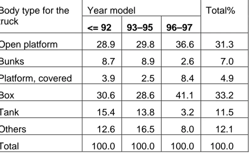
The objective has been to use a type of heavy truck vehicle body as common as possible in real traffic. Data from 1997 is available describing mileage for rigid truck (RT) and truck with trailer (TT/AT).6 Each such group is possible to split after type of vehicle body. In the group of heavy trucks and trailer with GVW>50 t mileage has been split after vehicle body (for the truck), see table 5.1.
Table 5.1 Distribution of mileage for HGV>50 t on type of body (1997).* Body type for the
truck
Year model Total% <= 92 93–95 96–97 Open platform 28.9 29.8 36.6 31.3 Bunks 8.7 8.9 2.6 7.0 Platform, covered 3.9 2.5 8.4 4.9 Box 30.6 28.6 41.1 33.2 Tank 15.4 13.8 3.2 11.5 Others 12.6 16.5 8.0 12.1 Total 100.0 100.0 100.0 100.0
*Tractor and trailer are not included.
Probably a substantial part of “open platform” and “others” in practice also are covered vehicles.
For rolling resistance the tyres used on the test vehicle are of interest. In Appendix A there is a detailed specification of test vehicle tyres. Conditions of special interest:
super single tyres on the trailer and ordinary tyres on the truck a mix of different tyre dimensions on the truck, see table A3 in total tyres from four different manufacturers, see table A3 tyre tread depth, see table A4
one tyre on the trailer was changed between first and second day of measurements.
The objective for tyres used in measurements was that they should be as common as possible on road vehicles.
The tyres on the test vehicle can be compared to observed frequencies of tyre type on trucks and trailers in general. Observed frequencies on parked trucks:7
Michelin 46% Dunlop 17% Kumho 9% Goodyear 5%
6 A data set used for (Hammarström and Yahya, 2000) has been analyzed further in order to estimate the
distribution of mileage on different vehicle bodies.
7 Observations on parking spots in Linköping and Norrköping 2009 in the VTI project
Yokohama 4% Semperit 4% Uniroyal 4% Continental 3% Bridgestone 3% Nordman 3% Nokian 2%.
Of 16 tyres in total on the test vehicle: 2 Michelin (12.5%)
8 Dunlop (50%) 4 Kumho (25%) 2 Yokohama (12.5%).
There have been two load conditions for the test vehicle: empty and approximately half loaded (20.4 t or lf=57%). In figure 5.1 and 5.2 the position of the load is described.
Figure 5.2 The position of the load in the trailer.
The tyre pressure is of importance for rolling resistance. The intention has been to set tyre pressure at stabilized tyre temperature conditions. Setting of tyre pressure:
driving axle: 7.5 bar other axles: 9.0 bar.
The tyre pressure needs to be adjusted to the specified pressure levels at least in the beginning of each measuring day. At the end of each day the pressure needs to be controlled.
For all measurements of tyre pressure there have been measurements of tyre
temperature in parallel. The tyre temperature also needs to be measured for systematic changes in measuring conditions like with and without trailer, different load conditions etc. The tyre temperature, the ambient temperature, and the air pressure can be used to estimate missing tyre pressure values.
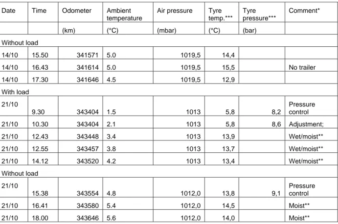
Measured tyre pressures are presented in table B1–B3 and measured tyre temperatures in figure B1–B6. In table 5.2 average tyre temperature and average pressure values are presented.
Table 5.2 Tyre temperature and tyre pressure at coastdowns for truck and trailer.
Date Time Odometer Ambient temperature
Air pressure Tyre temp.*** Tyre pressure*** Comment* (km) (°C) (mbar) (°C) (bar) Without load 14/10 15.50 341571 5.0 1019,5 14,4 14/10 16.43 341614 5.0 1019,5 15,5 No trailer 14/10 17.30 341646 4.5 1019,5 12,9 With load 21/10 9.30 343404 1.5 1013 5,8 8,2 Pressure control 21/10 10.30 343404 2.1 1013 5,8 8,6 Adjustment; 21/10 12.43 343448 3.4 1013 13,9 Wet/moist** 21/10 12.55 343457 3.8 1013 13,7 Wet/moist** 21/10 14.12 343520 4.2 1013 13,4 Wet/moist** Without load 21/10 15.38 343554 4.8 1012,0 13,8 9,1 Pressure control 21/10 16.41 343580 5.4 1012,0 14,5 Moist** 21/10 18.00 343646 5.6 1012,0 14,0 Moist**
*With trailer if nothing else is stated; **The wet or moist road surface was caused by high humidity i.e. not by rain;***Measured average values for all tyres. The averages with and without trailer are not comparable.
At measurements 14/10 practical problems with a tyre valve caused that there were no tyre measurements and no settings of tyre pressure.8
At measurements 21/10 the tyre pressure was handled as follows:
Measurement of tyre pressure for all tyres before adjustment, loaded vehicle Adjustment of tyre pressure: 7.5 and 9.0 bar respectively before coastdown,
loaded vehicle
Measurement of tyre pressure for all tyres after unloading and before measurements with unloaded vehicle.
Because of technical problems with tyre valves 21/10 the pressure settings were delayed and the pressure was adjusted at a tyre temperature below a driving stabilized
temperature level. After adjustment and conditioning the tyre temperature stabilized at a level of approximately 10.5 °C above the ambient temperature. After unloading and new conditioning the average tyre pressure was 0.5 bar above the desired pressure. The tyre pressure during coast downs 21/10 is estimated to be approximately 0.5 bar above the desired pressure level.
The wet road surface does not seem to have influenced the tyre temperature and probably not the tyre pressure either.
Based on ambient temperature, tyre temperature, air pressure and tyre pressure 21/10 the tyre pressure 14/10 has been estimated to be approximately marginally below the adjustment average level (the desired level)9. The resulting effect then would be that the tyre pressure during coastdowns at 14/10 can be closer to the desired level than at 21/10. The difference in pressure is estimated to be approximately 0.5 bar.
For rolling resistance the tread pattern depth is expected to be of importance. In table A4 the measured depth of the tread pattern per tyre is presented.
5.3 Measurement
equipment
For registration of the driving pattern in the coastdown an equipment VBOX 3i from Racelogic has been used, see Appendix C. VBOX measures speed and distance with a frequency of 100 Hz based on GPS. Speed is measured based on Doppler technique. Accelerometers are used in cases when the number of satellites in contact is insufficient. The equipment includes an antenna which has been mounted on the roof in the front of the truck box.
In order to connect the driving pattern with the road conditions, especially the gradient, there is a demand for high accuracy in the positions of the coastdown vehicle. In order to reach the desired accuracy a photo sensor on the vehicle is used. At the start coordinate and the end coordinate of the test route there is a reflector.
The registration of weather conditions is based on the following sources:
14/10: meteorological stations at Malmen airport and a VVIS station at road E4 21/10: one weather station placed close to the test route, see figure 5.3. The
height of the wind speed recorder was 1.5 m. Also data from Malmen and VVIS have been used.
Figure 5.3 Location of the meteorological station (21/10).
In order to have comparable wind speed data for the two days, recorded wind speeds in parallel at 21/10 from the different equipments were compared. Based on these data, observed wind speed from 14/10 was adjusted to be representative for the equipment used 21/10.
For tyre temperature measurements an infrared temperature measuring unit has been used. Temperature was measured in the centre of the tyre tread.
Tyre pressure was measured with equipment at a tyre company in Linköping. TheRoad Surface Tester (RST) has been used in order to measure road conditions
with exception for the road gradient, see picture 5.4.
Figure 5.4 The RST (Road Surface Tester) research vehicle is a multi-functional instrument.
Description of the RST:10
“Every variable can be measured simultaneously or independently. All measurements are made at normal traffic rhythm.
The variables are calculated and displayed in real time. Normally average data are stored and displayed every 20 metres, although this is adjustable from 5 metres upwards. Raw data can be collected if necessary. The results are produced in a well-defined file format. Alternatively VTI can analyse the data and deliver the results in the form of a report.
Cross profile
Cross profile is measured with the aid of up to 19 lasers and has a measuring width of 3.65 metres. Rut depth is calculated from the cross profile in accordance with the wire principle, both for the entire profile and for the right and left part.
Crossfall
The crossfall of the cross profile is measured as the inclination of the regression line for the cross profile and as the inclination of a fictitious line through two of the outermost lasers on each side.
Curvature
Curvature describes the mean curvature of the vehicle’s line of travel.
Longitudinal profile
Longitudinal profile is measured simultaneously in the left and right wheel track. At the same time, calculations are made of various roughness parameters such as IRI
(International Roughness Index) and RMS values for six different wavelength bands. This function of the RST was not used at Linghem test route.
Texture
Macrotexture and megatexture are measured simultaneously in the right wheel track and in the centre of the carriageway.”
Additional RST information for the Linghem test route: average data for 20 m sections
roughness: two detectors; one for the left wheel track and one for the right wheel track; distance between left and right, 1.50–1.52 m.
macro texture: three detectors; one for the left wheel track, one for the right wheel track and one between; distance between left and right, 1.50–1.52 m. The positions for iri and mpd measurement are a deficiency in order to estimate the influence on rolling resistance for a heavy truck. A distance of about 2 m would have been more representative in order to describe road surface effects for heavy trucks. One further deficiency is the width of each measured iri- and mpd track, just 0.5 mm. A width equal to the tyre width should increase the probability for measured road surface values being representative for tyre exposure.
The road surface measures by RST, measured per 20 m intervals, can be summarized as follows:
road roughness (iri) texture (mpd) crossfall (%) rut depth (mm).
In the ECRPD study the big importance of gradient data with high accuracy was demonstrated. In order to fulfil this demand gradients, altitude, were measured with levelling technique per 10 m. The gradient in between these 10 m observations was measured with laser equipment. These two data sets were matched together to give the complete vertical profile along the road.11
The levelling was done in one direction. For the other direction the gradient profile was mirrored.
5.4 The
test
route
The test route, see Appendix D, is situated in the community of Linköping, outside the urban area in an open landscape, see figure 5.5.
Figure 5.5 The test route in Linghem outside Linköping. General description of the test route:
length: 800 m both directions used
gradient (direction 1):12 - min: -1.0 (%)
- max: 1.2 (%) - mean: 0.21 (%)
average roughness both directions for the total data set: 1.2 (mm/m) (min: 0.65; max: 3.0)
average macro texture both directions for the total data set: 0.81 (mm) (min: 0.52; max: 1.0)
average crossfall:
- average direction 1:-3.1 (%) - average direction 2:-3.8 (%).
The road surface conditions on the test route are judged to be approximately representative for Swedish main roads.
5.5 Measurement procedure for coastdown
There have been measurements for three different vehicle modes, see table 5.3.
Table 5.3 Measurement modes and dates. The vehicle Unloaded Loaded Truck without trailer 14/10 - Truck with trailer 14/10;
21/10
21/10
There have been coastdowns from different initial speeds repeated three times each per mode (table 5.3) and road direction: 80; 50; 80; 50; 80; 50 km/h
Instructions for measurements:
Start with a full fuel tank per day if possible The road surface shall be dry
Average wind speed < 1 m/s if possible
Adjust tyre pressure to 7.5 bar on the driving axle and to 9 bar at other axles after conditioning until a stabilized temperature is reached
Check tyre pressure, tyre temperature in parallel, at least twice a day for warmed up tyres
Measure and document tyre temperature at least before and after each series of coastdowns
Measure the vehicle weight and note the odometer reading Side position: take a position in the centre of the wheel tracks
Accelerate to initial speed and put the clutch into neutral position before entering the start position of the test route
Begin the data collection before passing the start marking
If traffic is supposed to influence air resistance push the button marking not useful data
End the data collection after passing the end marking of the test route At the end of a measuring day fill the fuel tank up and make a note of the
odometer reading and the amount of fuel filled.
Special measurements like vehicle weight, tyre pressure etc. shall always have odometer reading in parallel.
To measure tyre pressure without changing the tyre pressure by leakage is not an easy task. The large number of tyres, 16 in total for the truck and trailer, contributes to the problem. The tyre pressure measurements have been performed by a tyre company in Linköping13. The same measuring unit was used for all tyre pressure measurements.
5.6 Meteorological
conditions
The conditions are described by using a weather station (21/10) placed approximately 10 m away from the road and 200 m away from the west endpoint of the test road, see figure 5.3.
For measurements 14/10 observations from nearby meteorological stations were used and adjusted to conditions representing the use of the described weather station. Wind speed and direction was registered on a height of 1.5 m.
In Appendix E meteorological conditions for each coastdown are presented.
The road surface conditions were not perfect at 21/10 since the surface was wet during the first part with loaded vehicle. The wet surface was caused by fog, i.e. not from rain. During the second part of the measurements the same day the surface was partly dry.
5.7 Measured
data
In Appendix E information per coastdown is documented including some important information like:
coastdown number date
speed at the start and at the end of each coastdown average dv/dt
ambient temperature meteorological wind speed
meteorological wind direction in relation to the vehicle movement direction ambient air pressure
ambient air moisture.
In Appendix E, figure E1–E8, all coastdowns are presented in diagram form. In table 5.4 number of coastdowns at different modes are presented.
Table 5.4 Number of coastdowns*
Unloaded Loaded Total
Truck without trailer (14/10): 8 0 8 Truck with trailer (14/10): 11
(21/10): 12
(21/10): 12 35
Total 31 12 43
*(xx/yy): date of measurements.
Per measuring mode the intention was to have 12 coastdowns: two directions; three initial speed levels and two coastdowns for each combination. The resulting numbers deviate from this intention especially for truck without trailer.
As a first approach the coastdowns have been split into 1 m long sections. The test route has a length of 800 m. Each coastdown results in 800 observations on aggregation level 1 m.
On aggregation level 25 m the number of observations is at most 32 per coastdown. Each such section, 1 m or 25 m, for each coastdown constitutes one observation in the analyse.
The data file for analyses has been reduced for observations with number of satellites: less than 8
higher than 15.
The reason for excluding observations with more than 15 satellites was that such a high number is an expression for an error.
The total number of observations (25 m) with trailer: without load, 686
with load, 361 total, 1047.
The total number of observations (25 m) without trailer: 243. Problems compared to intentions:
no tyre adjustments 14/10
considerable higher wind speed than should be accepted 14/10 moist road surface 21/10
not possible, for practical reasons, to measure tyre pressure for loaded and unloaded vehicle for the same conditions (21/10).
Since tyre pressure has not been adjusted in a desired way it is important to judge or estimate the variation in tyre pressure during measurements. If there is no leakage the tyre pressure should vary with the tyre temperature and the air pressure. There could also be an effect of tyre load at stand still.
For a constant tyre volume:
((Pw0+Pair0)/1000)/(Tw0+273)=((Pw1+Pair/1000)/(Tw1+273) Pw0: tyre overpressure at occasion 0 (mbar)
Pw1: tyre overpressure at occasion 1 (mbar) Pair0: air pressure att occasion 0 (mbar) Pair1: air pressure at occasion 1 (mbar) Tw0: tyre temperature at occasion 0 (°C) Tw1: tyre temperature at occasion 1 (°C).
This formula has been used in order to estimate tyre pressure at different occasions. There were no tyre pressure adjustments between 14/10 and 21/10. The tyre pressure 14/10 could be estimated based on the pressure 21/10 and on tyre temperature and air pressure both days. The estimated pressure 14/10 is then 2% below the desired values in average (7.5 and 9.0 respectively).
One question of interest is if tyre pressure changes as a function of tyre load for a tyre at constant temperature and air pressure at stand still. This is of importance in order to judge if there has been a leakage.
For practical reasons, in this project, tyre pressure could not be measured at the location where the load was changed. Because of this there will be different conditions for tyre pressure measurements with and without load. If the tyre pressures measured with load are adjusted for changes in tyre temperature and air pressure for conditions equal to those without load, the estimated tyre pressure is below the pressure without load. The difference between measured and estimated values is small, approximately 2%. The hypothesis was that the tyre pressure would be equal or decrease when the load decreased.
The ambient temperature at measurements without load 21/10 has been approximately 1.5 °C higher compared to measurements with load. The tyre temperature 21/10 without load has been 0.4 °C higher than with load. This difference in tyre temperature is caused both by the difference in ambient temperature and in load. The load is estimated to increase the tyre temperature with 1.1 °C.
One hypothesis could be that the driving axle tyres would have a higher temperature compared to the other axle tyres on the truck. In Appendix E it can be seen that this is not the case.
When looking at tyre temperatures for different axles the load per tyre could be of interest, see table 5.5.
Table 5.5 Tyre loads.*
Axle Tyres/axle Unloaded (N) Loaded (N) Truck 1 2 27125 35432 2 4 9712 20037 3 2 19424 40074 Trailer 1 2 12655 24550 2 2 12655 24550 3 2 12949 26242 4 2 12949 26242
*Values at the occasions for weight measurements 14/10 (unloaded) and 21/10 (loaded). The distribution between the second and third axle on the truck is based on the assumption that the total load per axle in the boogie is equal. Unloaded is measured 14/10 only. For the trailer the first two axles and the last two axles respectively are weighted together. The axle weight distribution in the front and in the rear of the trailer is based on the assumption of equal distribution.
A data set for the analysis has been prepared. This data set includes observed data for the different variables of interest. In the basic data set each coastdown has been split into observed values per meter. From this 1 meter level aggregation is possible to do for example to 25 m. The 1 m level is an aggregation of the measured data at 100 Hz. In order to develop driving resistance functions it is of importance to have high
correlations between the dependent and the explanation variables and in parallel not to have high correlations between explanation variables. In Appendix F correlation analysis is presented for two data sets, 25 m aggregation level only, restricted to measurements with trailer:
full data set
reduced data set (see below). Both data sets include the same variables.
The correlation includes variables: dv/dt; v; T; vl; Pair; fxl; dns; moist; gr; iri; mpd; crf and macc.
In total there are 66 correlation values between different variables other than dv/dt. The number of absolute correlation values in different size classes with exception for dv/dt in the total data set:
above 0.4: 13 above 0.5: 10 above 0.6: 9 above 0.7: 8.
The limit value 0.4 has been subjectively chosen.
The variables with absolute correlation values above 0.4 with exception for dv/dt combinations in the total data set:
fxl-v: 0.95 gr-v: 0.42 dns-temp: -0.68 macc-T: 0.86 Pair-vl: 0.97 dns-vl: 0.84 moist-vl: 0.95 dns-Pair: 0.89 moist-Pair: 0.97 moist-dns: -0.77 macc-moist: 0.51 mpd-gr: 0.43 crf-gr: 0.42
These correlations should be of special interest if the pair of variables is included in different explanatory variables in the analysis. In the road surface analysis there are some variables with a potential to cause problems. If a pair of variables with high correlation is included in the same explanatory variable there should not be any problem.
Because of the correlation between gradient and mpd, the basic data set has been adjusted:
observations with low gradient (downhill) and low mpd observations with high gradient (uphill) and high mpd. After reduction for gr-mpd correlation:
number of observations without load, 550 number of observations with load, 287 number of observations in total, 837 correlation gr-mpd: 0.132
correlation gr-v: -0.368 correlation crf-gr: -0.617.
For an analysis including gradient and mpd as independent variables the data reduction is necessary. For analysis not including mpd the basic data set should be used. The correlations after reduction of the data set are presented in table F4. In table F2 min and max and averages for different variables in the reduced data set are presented.
In Appendix E coastdown speed curves are presented, speed versus distance. One quality control of constant conditions from measurement to measurement is if the curves with the same start speed are parallel. In many cases, but not in all, they are parallel. If not parallel the reason should be possible to explain for example by different wind speed conditions. Coastdowns with different initial speeds should not be parallel because dv/dt is a function of v.
5.8 Examples of driving resistance parameter values from the
literature
Transmission losses
The churning losses have been estimated by functions documented in (Carlsson et al.,
2008):
Pvx= 5.1*(Prat/220000)*nr^1.62 Pbx= 10.08*((Prat/1000)^0.42)*nrk Pvx: gear box churning losses (W) Pbx: differential churning losses (W) Prat: engine max power (W)
nr: engine speed (rps)
nrk: rotation speed of the differential incoming axle (rps)
These functions are based on information from truck manufacturers.
For parameter values representing the coastdown truck one could expect transmission losses as presented in table 5.6.14
Table 5.6 Transmission churning losses for vehicle parameters representing the coastdown truck based on (Carlsson et al., 2008).
Unit Vehicle speed (m/s)
Notation 10 15 20 25 Differential Pbx..(W) 619 1194 1902 2731 Pbx/v..(N) 62 80 95 109 Gear box Pvx (W) 1649 2473 3297 4121 Pvx/v..(N) 165 165 165 165 Total (Pbx+Pvx)/v (N) 227 245 260 274
; *Direct gear position. During coastdown the gear has been in neutral position.
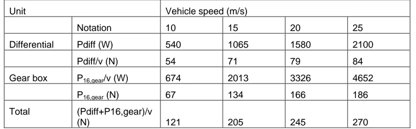
In (Rexeis, 2005) the sum of churning losses and mechanical losses are expressed in one function. There are separate functions for the differential (final gearbox) and the gearbox:
Pdiff = Prated ×0,0025×(−0,47 + 8,34× nwheel/nrat + 9.53 × ABS(Pdr/Prat))
Pdiff: total power losses in the differential (final gearbox) (W)
Prat: max engine power (W)
Pdr: power to overcome driving resistance (without transmission losses) (W)
nwheel: rotational speed of the wheels (rpm)
P16,gear=Prat*0,0025*(-0,66+4,07*(nr*60/(nrat*I16))+0,000867*abs(Pdr+Pdiff/Prat))
P16,gear: gearbox losses when the 16th gear is used nr: engine speed (rps)
nrat: engine speed at Prat (rpm)
I16: the gear ratio in gear position 16.
In order to estimate just churning losses with these functions Pdr and Pdiff are assigned
the zero value.
Table 5.7 Transmission churning losses for the coastdown truck based on (Rexeis, 2005).
Unit Vehicle speed (m/s)
Notation 10 15 20 25
Differential Pdiff (W) 540 1065 1580 2100
Pdiff/v (N) 54 71 79 84
Gear box P16,gear/v (W) 674 2013 3326 4652
P16,gear (N) 67 134 166 186 Total (Pdiff+P16,gear)/v (N) 121 205 245 270 Bearing resistance In (Mitschke, 1982) we have: Fb=Cb*Fz Cb=0.0005. Rolling resistance
In (Sandberg, 2008) rolling resistance values for trucks are reported: 215/70R22,5: -steered-wheel tyres: 0.0057–0.0063 - drive-wheel tyres: 0.006–0.007 315/80R22,5: - steered-wheel tyres: 0.0045–0.0055 - drive-wheel tyres: 0.0057–0.007
These values have been measured according to ISO 9948.15
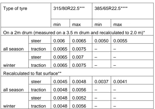
In (Siltanen, 2010) measured rolling resistance values on a drum are presented, see table 5.8.
15 Drum diameter: 1.7–3.0 m; test speed: 80 or 60 km/h; warm up: speed, 80 km/h and time: 90 or
Table 5.8 Rolling resistance values from drum measurements including recalculation to a flat surface for new tyres (Siltanen, 2010).
Type of tyre 315/80R22.5*** 385/65R22.5****
min max min max On a 2m drum (measured on a 3.5 m drum and recalculated to 2.0 m)*
all season steer 0.006 0.0065 0.0050 0.0055 traction 0.0065 0.0075 – – winter steer 0.0065 0.007 – – traction 0.0065 0.0075 – – Recalculated to flat surface**
all season steer 0.0045 0.0048 0.0037 0.0041 traction 0.0048 0.0056 – – winter steer 0.0048 0.0052 – – traction 0.0048 0.0056 – –
*ISO 28580; **Recalculation based on (Mitschke, 1982) 16;***8.25–8.5 bar depending on load index;
****8.5–9.0 bar depending on load index.
Approximately 30% of the rolling resistance for a new tyre is caused by the tread. The rolling resistance for worn out tyres is then estimated to be 30% lower compared to table 5.6.
In (Reithmaier et al., 2000) rolling resistance values measured on a drum are presented. Description of the measurements:
ISO 9948
drum diameter: 1707 mm
conditioned at least 6 h under test room conditions
tyres are run under test conditions for 120 minutes at 80 km/h before measurements
16Function for estimation of rolling resistance on a flat surface based on measurements on a drum
(Mitschke, 1982):
FR,T/fR,E = (1 + (2 x rwh)/D)0,5 where
D is the diameter of the drum (m)
FR,T is the rolling resistance on a drum (N)
FR,E is the rolling resistance on a flat surface (N)
the tyre pressure is adjusted on the conditioned tyre, during measurement tyre pressure can build up freely
test room temperature: 25 °C
the rolling resistance is calculated by using a formula in ISO 9948 two tyres are measured from each manufacturer and dimension.
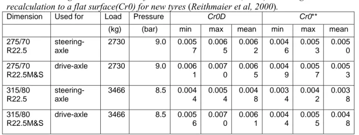
Table 5.9 Rolling resistance values* from drum measurements (Cr0D) including recalculation to a flat surface(Cr0) for new tyres (Reithmaier et al, 2000).
Dimension Used for Load Pressure Cr0D Cr0**
(kg) (bar) min max mean min max mean 275/70 R22.5 steering-axle 2730 9.0 0.005 7 0.006 5 0.006 2 0.004 6 0.005 3 0.005 0 275/70 R22.5M&S drive-axle 2730 9.0 0.006 1 0.007 0 0.006 5 0.004 9 0.005 7 0.005 3 315/80 R22.5 steering-axle 3466 8.5 0.004 4 0.005 4 0.004 8 0.003 4 0.004 2 0.003 8 315/80 R22.5M&S drive-axle 3466 8.5 0.005 6 0.007 0 0.006 1 0.004 4 0.005 5 0.004 8
* ISO 9948; **Estimated based on (Mitschke, 1982).
To summarize one can notice more than minor difference in Cr0 between different literature sources (dimension 315/80R22.5). Drive axle Cr0D is always at least as high as the steering axle.
There is information in the literature about Cr being a function of the vertical load Fz
(Rexeis et al., 2005):17 Cr = Crz0 – Crz1 x Fz/1000 Crz0 = 0.00825 Crz1 = 0.000075 where Fz: vertical load (N)
Crz0 and Crz1 are constant parameters.
This means that the rolling resistance (Fr) depends quadratic on Fz.
Based on this function rolling resistance (Cr) has been estimated for different segments of HGV, see table 5.10.