The longevity of cars in Sweden

% l/TIratt E

321 A

1.987

The longevity of cars in Sweden

1965 - 1984

Bernard P. Feeney and Peter Cardebring

(db

_{Vag- 00/)}

_{Statens vé'g- och tre kinstitut (VT/l - 58 1 0 1 Linkb'ping}

l/TIratmt:

321 A

1937

The longevity of cars in Sweden

1965- 7984

Bernard F. Feeney and Peter Cardebring

(db

Vag- 00/1

Statens ve'g- och trafikinstitut (VT/l - 58 1 0 1 Linkb'ping

lllStltl/tet Swedish Road and Traffic Research Institute o 8-58 1 o 1 Lin/taping Sweden

FOREWORD

This study was carried out in close co-operation with Statistiska Centralbyrgn (The Swedish Central Bureau of Statistics). The authors acknowledge with thanks the invaluable and efficient help which they received from Mr. Folke Carlsson of that organisation.

TABLE OF CONTENTS

ABSTRACT SUMMARY

1. INTRODUCTION

2. A REVIEW OF PREVIOUS ESTIMATES AND METHODOLOGIES

2.1 Swedish Estimates

2.2 International Estimates

3. DATA PROBLEMS

3.1 Inaccuracies in Car Fleet Statistics

3.2 Classifying the Car Fleet

3.3 A Methodology for Estimating the Level

and Structure of the Passive Car Fleet 3.4 Results

4. CAR LONGEVITY

4.1 Alternative Forms of Survival Functions

4.2 Estimates of Car Longevity

4.3 Comparisons with Other Estimates

5. CONCLUSIONS REFERENCES

APPENDIX 1: Median Life Expectancy of Cars

in the USA Al. Introduction

A2. Methodology and Results

VTI RAPPORT 321A

Page II 10 11 22 25 25 28 3O 35 39 42 42 42

The Longevity of Cars in Sweden 1965-84 by Bernard F. Feeney and Peter Cardebring

Swedish Road and Traffic Research Institute (VTI) 5-58101 LINKOPING, Sweden

ABSTRACT

Previous studies have tended to exaggerate car longevity in Sweden. This has arisen because of the inclusion in the car fleet of vehicles which are no longer roadworthy. This report makes estimates of the true car fleet for the period 1965-84 disaggregated by age and make. Based on these estimates survival functions for cars are established. The mean life expectancy of cars is estimated at 14.7 years for 1984, as compared with 9.# years in 1965. This is some 2 years below previous estimates. However, mediancar life in Sweden is still 1 year above that for the U.S.A., for example.

II

The Longevity of Cars in Sweden 1965-84 by Bernard P. Feeney and Peter Cardebring

Swedish Road and Traffic Research Institute (VTI)

5-58101 LINKOPING, Sweden

SUMMARY

The longevity of the car fleet has important implications for the size and structure of the car market, the measurement of depreciation charges to be assigned to vehicles and the rate at which changes in technology and legislative actions, aimed at new cars, pervade the total car fleet. This report presents estimates of the life expectancy of cars in Sweden for the period 1965-1984.

Previous studies have tended to exaggerate car longevity in Sweden. This has arisen because of the inclusion in the car fleet of vehicles which are no longer roadworthy. Cars may be registered either as "i trafik" (active) or "avstalld" (passive). However passive carsmay be either temporarily passive and, therefore, available for use, or permanently passive or scrapped. This study develops a methodology for estimating the number of temporarily passive cars and their joint age, make and size distribution. It is established that for the year 1984, out of a total of 3,712,000 cars in the register, 436,000 are permanently passive. Thus, the true car fleet,

available for use, was 3,276,000 of which 195,000 were temporarily

passive. As previous estimates of car longevity were based on the total car register, active plus passive, they have been seriously in error.

The number of passive cars began to grow quickly from about 1973, when charges for moving a vehicle from active to passive status were abolished and the procedure was also simplified administratively. Thus, relatively speaking, it became easier to make a car passive than to deregister it completely, and this gave rise to an increasing pool of permanently passive cars. The number of temporarily passive cars also began to grow strongly from about 1977, because of increases in the vehicle tax and changes in the administrative arrangements relating to insurance. Of the total of 195,000 temporarily passive cars in 1984, approximately 56,000 were habitually wintered, while the bulk of the remainder were in the

III

course of being traded. The probability that a car will be made temporarily passive is greater for older vehicles and non-Swedish makes. Having estimated the size and structure of the true car fleet for the period 1965-84, logistic survival functions were calculated for each year using non-linear regression estimation techniques. The median life expectancy was then estimated at 14.7 years (1984) which is some 2 years below previous estimates. It was established that median life expectancy grew strongly in the period 1965 73, declined slightly thereafter, and resumed its upward trend in 1978. Comparisons with median life expectancy of cars in other countries is made difficult because of the different measurement methodologies and data time periods used. However, a comparable analysis of car longevity in the U.S.A. shows that car median life expenctancy is 1 year below the Swedish level.

This study has several implications for statistical policy and transport research. Firstly, it is apparent that neither of the two official measures of the Swedish car fleet accurately reflect the true number of cars available for use on the road. There is thus a need for Statistiska Centralbyran to provide a third and more accurate measure of car numbers on a continuing basis. Secondly, this study has considered cars in the aggregate, whereas car longevity is known to vary considerably by make. An extension of the study to measure life expectancies for different cars makes and sizes is warranted. Thirdly, further research is required to investigate the relative importance of car age, technical characteristics, economic conditions and legislative actions in determining car scrapping behaviour.

1 . INTRODUCTION

The longevity of the car fleet has important implications for the size and structure of the car market, the measurement of depreciation charges to be assigned to vehicles and the rate at which changes in technology and legislative actions, aimed at new cars, pervade the total car fleet. This report presents estimates of the life expectancy of cars in Sweden for the period 1965-84.

In. common. with similar studies, life expectancy' is estimated by examining the age distribution of vehicles in the car register. A special problem arises in the Swedish context because of the twofold classification of vehicles within the register: a Vehicle may be registered either as 'i trafik' (in use) or 'avstalld' (not in use). Cardebring and Jansson (1985) have shown that of the total of cars not in use only one-third become active again. It is, therefore, wrong to assume that a vehicle's time of 'death', that is the point in time when it is no longer available for use on the road system, coincides with its deletion from the car register. Thus, before any life expectancy estimates can be made, the age distribution of the 'true' car fleet must be estim-ated. Secthma 3 of this report deals with this problem, while survival functions and life expectancies are calculated in Section 4. Prior to this, however, a review of previous life expectancy estimates and the methods employed is presented in

Section 2.

2 . A REVIEW OF PREVIOUS ESTIMATES AND METHODOLOGIES

2.1 Swedish Estimates

Previous estimates of car life expectancy in Sweden have been made by AB Svensk Bilprovning (The Swedish Motor vehicle Inspection Company) and published in a series of reports (see for example, AB Svensk Bilprovning 1972 and 1975). The methodology used was to first calculate age-specific scrappage rates q(x), by comparing the vehicle register at two successive end-years:

t X l

where qt(x) is the annual scrappage rate for x year

. 1:

old cars 1n year t, and Nt_x_1

of cars first registered in year t x-l still in represents the number existence at the end of year t.

The proportion of cars surviving to age x (Pt(x)) was

then calculated as

Pt(x) = 11:: (l - qt(x)) (2.2) In this method, which is the one normally used in human life table estimation, survival proportions are based on age-specific scrappage rates derived from the most recent vintage of vehicle achieving that age. Thus, the life expectancy estimates do not refer to vehicles of any specific vintage. This may be called the variable vintage method. The alternative approach is to measure the survival proportions of a cohort of

vehicles first registered 3 years ago, by examining scrapping from that cohort over the intervening period - the fixed vintage method. Thus, if an 3 year survival function is to be estimated in year t, the survival proportion is calculated as

Nt-s+x - t-s

Pix? = E:g * _(2-3)

Nt-s

where Pt-S(x) is the proportion of the fleet first registered in year t-s which survives to age x years

t s+x

t_s t-s .

year t-s surviving to year t-s+x, and Nt_s 18 the is the number of vehicles first registered in total number first registered in year t-s. However, this has the drawback that an adequate description of the survival function may be obtained only after a large number of years has elapsed, and the survival function thus obtained may be a poor indicator of the longevity of the current car fleet. It should also be noted that while the variable vintage method produces estimates which are open to the influence of economic conditions in the current year t, the fixed vintage method reflects economic conditions over the past 5 years. The survival functions calculated by AB Svensk Bilprovning were not given mathematical form, but were typified by time median life expectancy calculated by interpolation. The median life expectancy of Swedish cars was found to increase from 9.4 years in 1965 to 16.2 years in 1982. The most substantial increase took place during the period 1971-73 when an increase of 2.0 years was recorded. Part of the reason for this lies undoubtedly in the fact that prior to 1971, the calculations were based.<n1 cars in use, whereas

from 1973 onwards cars not in use were also included*.

* AB Svensk Bilprovning do not provide an estimate for 1972.

By 1982 there was serious doubt as to whether the inclusion of all cars not in use was justified and no further calculations were made.

Median life expectancies were also estimated by AB Svensk Bilprovning for the principal car makes. A feature of the results was the superior performance of Volvo cars; for 1982 their median life expectancy was almost 21 years, or almost 30 per cent above the average.

2.2 International Estimates

Given the importance of the subject, it is surprising that there is relatively little international research published on car longevity. What is available falls into two categories: the first deals with the estimation of mathematical survival or age - specific scrappage rate functions, while the second deals with examining the determinants of year to year changes in

scrappage rates.

Thoresen and Stella (1977) for Australia, Ernvall (1983) for Finland, Bennett (1976) for Great Britain and Cramer (1958) for both the United Kingdom and the U.SHA. all estimate mathematical survival functions. Both Ernvall and Cramer use variable and fixed vintage methods to calculate survival functions, which are then expressed mathematically using the logistic function in the former and the Gompertz in the latter. Median life expectancies ranging from 10.4 years (1971) to 13.2 years (1982) are measured by Ernvall for Finland using the 'variable vintage 'method, and 13.5 years (1969) using the fixed vintage method. Cramer worked with considerably older data and calculated mean life expectancies of 8 to 9 years for the U.K. (1936-38) using the variable vintage method

and 10 to 11 years for the U.S.A. (1930-42) using the fixed vintage method. Both Thoresen and Stella and Bennett had only one year's age distributions to work with, so Pt(x) was calculated from a knowledge of the age distribution of the car fleet in year t and the total number of cars registered in each year prior to

t: t

Pt(x) = Nt-x

(2.4)

t-x Nt-x

where Ntt_x represents the number of cars first registered in year t-x and still in existence in year t. This may be called the approximate variable vintage method. It suffers from the disadvantage that the results can be related neither to a fixed vintage

of cars or to annual economic conditions.

Thoresen and Stella fitted a logistic function and Bennett a negative exponential function; a median life expectancy of 13.6 years for Australia (1971) and a mean life expectancy of just under 12 years for Britain (1974) were established. Greene and Chen (1981) estimate annual age-specific scrappage rates on U.S. data for the years 1966-77 using formula (2.1). After.fitting a scrappage rate logistic function, they estimate a survival function covering the entire period. Thus, although they use the variable vintage method, the results are averaged over an eleven year period. A median life expectancy of just under 10 years is calculated. Other related studies are those of Parks (1977), Walker (1968) and Manski and Golden (1983) who are not directly concerned with the estimation of survival or scrappage rate functions but with gestablishing the determinants of scrapping

behaviour.

Ignoring Cramer's estimates which relate to a now distant time period, the calculated life expectancies range from 10 years for USA to over 16 years for Sweden. However, given the very different measurement methodologies and data time periods, and the use of both mean anui median life expectancies, too much should not be made of such differences. In addition, as indicated above, the Swedish results are further complicated by the inclusion of currently inactive vehicles which will never become active again. The purpose of this study is to provide a more accurate estimate of Swedish car life expectancy and, if possible, make a valid comparison with data from other

countries.

3 . DATA PROBLEMS

3.1 Inaccuracies in Car Fleet Statistics

A special feature of the Swedish registration system is that vehicles are not required to be continuously taxed and insured. This provision arose, in the first instance, in the early 19203 when it was recognised that because of the relative severity of the Swedish winter, many cars were simply unusable for several months of the year. The inequity of taxation without possibility of use led the authorities to introduce a two-tier registration system, in which vehicles could be registered as 'in use' or 'not in use'. For ease of reference, vehicles in these categories will be referred 1x) as 'active' and. 'passive' respectively. Active cars (A) must pay the Fordonskatt (annual vehicle tax) apprOpriate to their taxation class and must be currently insured; passive cars (P), on the other hand, are entitled to tax and insurance refunds for the period of time for which they are passive. This dual system was reviewed in 1971 (300, 1971) and retained principally to allow commercial vehicle owners to continue to obtain tax refunds for vehicles in periodic use. The review body retained the system for private cars also, believing that their use of the passive status would be Iknv or confined to some special cases. While the original intention of the legislation was to allow vehicles to be wintered, they can be rendered passive for other reasons, too: if, for example, vehicles are undergoing repair of a long term nature, or if the vehicle owner is suffering from a lengthy illness, or going abroad for an extended period.

The use made of this flexibility in the registration system was not, until recently, substantial. In 1960, for example, only 52,300 cars, or 4 per cent of the car fleet, were registered as passive. By 1970, the equivalent figures were 134,300 and 5.5 per cent. The most substantial increase in the number of passive cars took place during the 1970s: in 1977, the numbers rose by 123,300 to 337,900 and in 1979 by 60,500 to 450,900. By 1984, the total number passive stood at 631,000 or 17 per cent of the car fleet.

These increases in the passive car fleet can be traced to a number of changes in the registration, tax and insurance systems relating to vehicles. Firstly, following computerisation and centralisation of the vehicle register in 1972, the administrative charges for moving a vehicle from active to passive status, and vice-versa, were abolished, and tax refunds were automatically forwarded rather than requiring a special written application on the motorist's part. Secondly, in 1979, insurance practices were changed with the result that car dealers were charged in relation to the number of days in which vehicles in their possession were in use and not on the basis of the total annual number of vehicles passing through their hands. Thirdly, also in that year, the Fordonskatt levied on cars was increased by almost 75 per cent. As a result of these changes, the financial incentive to make a car passive was increased and the administrative difficulty of doing so was reduced. The increasing number of passive cars would not, in itself, constitute a problem for the estimation of car longevity provided such cars eventually returned to active status. However, Cardebring and Jansson (1985) have assembled substantial evidence to show that this

is not the case. By examining vehicle flows to and from the active register for the period 1976 to 1982,

they estimated that of a total of 631,000 passive cars in 1984, 243,000 would eventually be brought back into active status; of the remainder, 100,000 would eventually be deregistered while another 300,000 were likely to remain in the passive register indefinitely, unless removed by administrative flat. The existence of this latter category of vehicles can be attributed to the ease at which vehicles could be made passive and the relative difficulty of deregistering them.* Thus, of the total passive, only just over one-third return to active use. The implication is that neither of the two alternative and readily available measures of the car fleet - the active fleet (A) and the total - active plus passive - fleet (T) is a good indicator of the true car fleet which is available for use (Tu). To obtain an estimate of the true car fleet, one must add the temporarily passive Pt to the active, i.e.

U pt (3.1)

Cardebring and Jansson used this approach to reconstruct a series to represent the true development of the car fleet over the period 1976-1984. This was subsequently used as an input to a car forecasting model for Sweden (Jansson, Cardebring and Junghard,

1986). This series showed that since 1976, the diver-gence between the active car fleet and the true car fleet had grown from 80,000 vehicles to 243,000 by 1984. These inaccuracies in the car fleet statistics * In order to deregister a vehicle, the owner must

prove that the vehicle no longer exists, usually 'by obtaining a certificate from an authorised scrapyard. This may involve costs of transporting the vehicle to the scrapyard.

10

indicate that neither the active nor the total fleet are suitable for the purposes of measuring car longevity. Previous estimates CHE median life expectancy have, most recently, been based on the total car fleet, and have, therefore, tended to over-estimate car life expectancy during the late 19705 and early 19803.

3.2 Classifying the Car Fleet

Measurement of the age distribution of the true car fleet requires a definition of car age. Ideally, it would have been desirable to measure age by time elapsed from initial registration, as the time of birth of individual or categories of cars could then be identified as lying within a particular calendar year. However, for the period prior to the computerisation of the car register in 1972, data on the car fleet by year of first registration are not available. Consequently, 'model year' was used to

determine time of birth.

While knowledge of the model year distribution of the true car fleet for the period under analysis would permit the estimation of overall car longevity employing any of the methods outlined in Section 2, it was thought useful to extend the analysis to enable the investigation of how car longevity varies with car make and size» It was recognised at the outset that

to estimate Pt through a complete three-way classification of the true car fleet by model year, make and size was impractical, and that make and size needed to be limited to a small number of categories. Analysis of new car sales over the period 1960-84 revealed that five makes - Volvo, Saab, Ford, Opel and Volkswagen accounted for two-thirds to three quarters of all new car registrations. Thus, six make

11

categories, includimg a catch-all 'other' make, were identified. Six size classes based on service weight*

were identified as follows:

0 - 999 kilograms 1,000 - 1,099 " 1,100 - 1,199 " 1,200 - 1,299 " 1,300 - 1,399 " 1 1,400

These were chosen so as to ensure an adequate number of cars in each category over the analysis period. A threeway classification of the active car fleet by the above model year, make and size categories -was found to be feasible for the period from 1973 only, when the computerised register commenced. For the years prior to this, a model year by make

classification is available.

3.3 A Methodology for Estimating the Level and

Structure of the Passive Car Fleet

In order to obtain data suitable for the estimation of car longevity, it was necessary to describe a three way classification (by model - year, make and size) not only for active cars (A), but also for temporarily passive ones (Pt). Cardebring and Jansson (1985) estimated the total number of passive cars by examining the size of flows to and from the active .register, and by applying a set of factors to determine the vehicular mix of such flows. As analysis of these flows could not be extended to identify model-year, make and size characteristics, an

* The weight of the vehicle ready to use, fitted with the heaviest body belonging to it including the weight of tools, spare wheel, fuel, lubricating oil, water and the driver.

12

alternative approach was developed based on an examination of the car register at successive year-ends. In addition to comprehensive data relating to the characteristics (Hi the car (weight, length, fuel used, number of doors, tyre dimensions etc) and more limited information relating to the owner (name, address, private or company) the computerised vehicle register also contains data on the registration status of the car (active or passive) and date at which the car became passive. Thus, it is possible to identify, for a particular year end, which cars are passive and when they entered passive status.

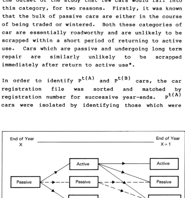
In order to identify temporarily passive cars, it was necessary to determine whether cars, which were registered as passive at a particular year-end, subsequently returned to active status. The obvious approach is to compare vehicle registers at successive year-ends and identify those cars which were passive at the first year-end but active at the subsequent one. However, it is possible for cars to become active during the course of the year, but to have changed status again tug the year~end. Figure 1 depicts the principal alternative registration patterns for passive vehicles over the space of one year. The continuous lines represent the registration patterns which are CHE interest for the detection of temporarily passive vehicles. In addition to those passive cars which become active during the year and remained so (Pt(A)) others may have become active but returned to passive status by the next year-end

(pt B ).

exhibit this behaviour. Another possibility is that Cars which are habitually wintered would cars passive at (nu; year-end might become active during the year but would be subsequently deregistered

t(C)).

before the next year-end (P It was decided at

13

the outset of the study that few cars would fall into this category, for two reasons. Firstly, it was known that the bulk of passive cars are either in the course of being traded or wintered. Both these categories of car are essentially roadworthy and are unlikely to be scrapped within a short period of returning to active use. Cars which are passive and undergoing long term repair are similarly unlikely to be scrapped immediately after return to active use*.

t(B)

HA) and P cars, the car

In order to identify P

registration file was sorted and matched by registration number for successive year-ends. iPtLA) cars were isolated by identifying those which were

End of Year End of Year

X X+1

Active > [L Active I

Passive + l Passive + -- Passive J \

\ \

_ A \\

Deregistered l -> - - Deregistered l

Figure 1. Alternative Registration Patterns for Passive Cars.

t(C) *' An estimate of the number of cars in the P

category was made for one year, 1985. It was established that only 3,300 cars fell into this

category.

14

passive at the first year-end and active at the

second. Pt(B) cars were determined by isolating those which were passive at both year-ends but had been active between those year-ends. This was done for each cell in the age, make and size

cross-classification.

The above method encompasses cars which return to active status within one year of a particular year-end. Cardebring and Jansson have shown that typically only 13 per cent of temporarily passive cars do not return within one year. Accordingly, the total of temporarily passive cars Pt was obtained by factoring up the sum of Pt(A) and Pt(B), i.e.

3.2)

t _

1

t(A)

t(B)

(

P

i3Fk 1 9 (Pijk + Pijk)

where e is the proportion of cars returning after one year as determined by Cardebring and Jansson and i, j and k refer to age, make and size respectively*. The true car fleet was then estimated as

TU = A + Pt

(3.3)

The validity of factoring by T%§in the context of estimating car longevity rests on the supposition that the age distribution of the temporarily passive cars returning after one year is similar to that of those returning within one year. This raises the question of whether the age structure of temporarily passive cars is independent of the length of time for which they are passive. Some evidence relating to this could be gleaned for the period 1984/85 by comparing the age structure of those cars which were passive at

6 varied from a low of 11 per cent for 1979 to a high of 21 per cent for 1976.

15

end 1984 and which had become active by July 1985 with the age structure of those returning to active status-between July and December 1985*. The average age of the two groups proved identical at 10.4 years. While examination of the age distributions showed that July-December cars tended to be relatively under-represented at both older and newer model year groups, the discrepancy is not sufficiently large as to produce substantial inaccuracies in the estimated age

distribution of Pt, much less that of TU cars (see

Figure 2). per cent

A}

figure_3. Model Year Distribution by Period of Return to

Active Status.

T This could be done for 1984/85 only as the July file of the car register is retained for a short period only.

16

Using the above procedure the number of temporarily passive cars for 1984 was estimated to be 195,000 or 31 per cent of the passive car fleet. This can be compared. with Cardebring and Jansson's estimate of 243,000 cars or 38 per cent of the passive car fleet. Thus, of time total of 3,756,000 registered cars, 3,081,000 were active, 195,000 temporarily passive and 436,000 permanently passive or scrapped. Of the total of 195,000 temporarily' passive, 56,000 are (HE type Pt(B) and this is an approximate measure of the number habitualLy wintered*. Of the remaining 139,000 the bulk are probably in the course of being traded: this view is supported by a separate analysis of the passive register by owner type which revealed that, over the period 1982-84 on average, approximately 85,000 were owned by motor dealers (Cardebring (1987)). The variathmn in the proportion of temporarily passive by make is given in Table 1 which also gives corresponding figures for the years 1981, 1982 and 1983. The overall proportion of temporarily passive cars has been stable over these years, while the domestic makes - Volvo and Saab - consistently exhibit a lesser tendency to be made temporarily passive. Table 2 gives details of Pt I 3:121. and Pt(:) by model-year. The most striking featgre of the tgble is the sharp decline ix: %; among younger vehicles - a result which is almost entirely due to a

t(B)

I I O O P I O 0

Similar decline in ._ r_ . This implies that the probability of a car being 'wintered' increases sharply with age, but the corresponding increase for traded cars is considerably less.

*7 In what follows Pt(B) cars are referred to as 'wintered'. However, it should be recognised that PHB) excludes cars which are wintered one year but not the next. It also may include a small number of cars which are wintered at one year-end but are in the course of being traded at the next year-end.

17

TabTe 1. PrOportion of True Car FTeet which is TemporariTy Passive by Make and Year (1981-84).

MAKE YEAR 1981 1982 1983 1984 (%) (%) (%) (%) VOLVO 4.32 4.56 4.92 4.00 SAAB 4.38 4.39 4.18 4.21 FORD 7.46 7.55 6.81 6.12 OPEL 5.89 6.08 5.67 5.36 VOLKSWAGEN 5.96 7.84 7.31 8.26 OTHER 8.59 8.85 8.19 8.13 TOTAL 6.11 6.48 6.21 5.93

TabTe 2. _{Pr0p0rti0n of The True Car FTeet which is TemporariTy} Passive, by ModeT Year (1984).

MODEL

PROPORTION OF CARS TEMPORARILY PASSIVE

YEARS

Pt(A)

Pt(B)

Pt

U

U

0

T

T

T

5_1955

5.5

37.5

43.0

>1955 g_1960

5.0

21.5

26.5

>1960 5_1965

4.5

10.2

14.7

>1965 5_1970

4.6

8.6

13.1

>1970 5_1975

2.3

2.6

4.9

>1975 £_1980

2.5

0.9

3.4

>1980 5_1985

3.4

0.3

3.7

TOTAL

2.9

2.2

5.1

Note: Refers to cars passive at the end of December 1984 and returning to active status before the end of December 1985. VTI RAPPORT 321A

18

The above procedure was employed to derive estimates of the true car fleet for the years 1981-84 inclusive. The procedure could run: be applied 1x) the years 1973-80 because only an abbreviated vehicle file was kept, which did not contain a record of the date at which the car was made passive. Therefore, Pt(A)

but not Pt(B)

used for this latter time period was to establish a cars cars could be identified. The approach set of factors 'Y representing the conditional probab-ility of a temporarily passive car being wintered,

. FJB) . U .

1.e. v'=- Eg-and to estimate T by applying these

factors to the known level of FHA). Table 3 shows

values of y for each make for the years 1981-84. Saab, Volvo and Opel have a below average probability of being 'wintered', while Ford, Volkswagen and other makes are above average. In general, one in three temporarily passive cars are 'wintered'. With the exception of Volkswagen, all makes exhibit remarkable stability in Y over the period.

Table 4 presents values of Y for 1984, differentiating by make and model year. For model years prior to 1975, VOlvo exhibits the lowest probability of being wintered, while for the remaining model years, Saab is lowest. Overall, Saab has the lowest probability of being 'wintered' at 15.2 per cent, which suggests that this make has a higher proportion of young temporarily passive cars (i.e. (HE recent model years) than does Volvo. It is not possible to say precisly why Swedish makes exhibit this characteristic. However, the

tend-ency for Swedish car manufacturers to concentrate on

the large quality vehicle segment of the market may mean that their vehicles are better equipped, on

aver-age, to withstand winter conditions. Additionally,

the Swedish makes are more likely than their foreign

19

Tab1e 3. 'Wintered' Cars as a Pr0p0rtion of T0ta1 Temporari1y Passive Cars by Make 1981-1984.

MODEL MAKE YEAR

Volvo Saab Ford Opel V'wagen Other Total

% % % % % % % g 1960 60.1 71.7 81.0 72.4 65.9 79.5 73.3 >1960 g 1965 40.8 52.6 72.9 57.9 64.9 76.5 61.6 >1965 g 1970 31.3 35.0 70.4 45.20 65.4 71.8 56.0 >1970 g 1975 20.5 21.0 37.1 28.2 34.8 46.0 34.9 >1975 g 1980 14.0 9.7 16.2 16.5 15.9 22.0 17.6 > 1980 5.6 4.5 6.9 6.2 6.6 10.4 7.4

TOTAL

23.3

15.2

37.9

'27.6

38.9

41.9

33.4

Tab1e 4. 'Wintered' Cars as a Pr0p0rti0n of Tota] Temporari1y Passive Cars by Make and M0de1 Year for 1984.

MODEL MAKE YEAR

Volvo Saab Ford Opel V'wagen Other Total

% % % % % % % 1981 24.8 16.4 37.9 28.4 30.8 41.8 32.9 1982 23.4 16.6 36.0 27.0 34.8 40.9 32.4 1983 22.8 15.9 36.7 26.8 39.1 42.1 33.2 1984 23.3 15.2 37.9 27.6 38.9 41.9 33.4 SIMPLE 23.6 16.0 37.1 27.5 35.9 41.7 33.0 AVERAGE

20

counterparts to be used as company cars (Cardebring, 1987), and this implies continuous use throughout the year.

. . Pt(B) .

The above analy51s established that It varies P

considerably across makes and model years. Accord-ingly, on the basis of the 1981 data, a set of factors

. t(B)

Yijwas established to measure the quantlty .B_Ef_for a matrix of 36 model year classes by 6 make classes, and

t(A) these were used to factor up the quantity P for each of the 216 classes for the years 1978-80. The familiar adjustment for temporarily passive cars returning after more than one year was then added:

t _ l tJA) l

P -'3% 1-6 (Pij ' l yij ) (3.4) where i refers to 36 model year classes and j refers

to six make classes.

Initially, a three-way matrix of factors to include 6 weight classes was calculated. However, this resulted in many cells which were either zero or based on very small numbers, so that the above two-way classific-ation was finally adopted. This procedure provided a basis for extending the calculation of TU back to 1973. The results are presented in Table 5. It can be seen that in 1973, the number of temporarily passive cars was approximately 76,000 or 3 per cent of the true car fleet. This implies that the use of the active fleet as the basis for measuring car longevity for the period prior to that year would not lead to

serious inaccuracies. However, in order to yield

estimates for 1965-72 consistent with those for the later period, the number of passive cars in the former period was estimated by applying the factor Q to the active fleet in the following manner

21

TU = 2A.. L

1]

(3.5)

(i) and make (j) is temporarily passive.

The factor pij was not based on year 1973, because it was felt that this year had witnessed a higher than usual level of temporarily passive cars (76,000 as opposed to 61,000 to 65,000 in subsequent years) due

to a number of factors: firstly, the abolition of the

charges for making ea car passive, together with the increased ease of doing so following computerisation may have induced some motorists to experiment temporariLy with wintering their vehicles; alternat-ively, the fuel price increases and uncertainty concerning fuel supply which was present during 1973-1974 may have encouraged motorists with marginal motoring needs to make their vehicle passive. In either case, it is likely that 1973 is an atypical year and does not give a good indication of registration behaviour prior to that year. While there is.ru> way of determining with accuracy the number of temporarily passive cafs for the period prior to 1973, a crude estimate can be made by assuming that the probability of a car of a given make and age being temporarily passive pij is the same as in 1974. The results for the period 1965-72 are

presented in Table 5, where it is estimated that in

1965 only 30,000 cars or less than 2 per cent of the true fleet was temporarily passive.

22

3.4 Results

TabLe 5 shows that, in 1984, there were an estimated 3,2760,000 cars available for use in Sweden*. As the total car fleet comprising active plus passive vehicles was 3,712,000 vehicles, this implies that 436,000 registered cars must be regarded as perman-ently passive or scrapped. The total of 3,276,000 cars available for use is made up of 3,081,000 active and 195,000 temporarily passive vehicles. Since 1965, the number of temporarily passive cars has increased sixfobd and the number of permanently passive or scrapped sevenfold. The number of permanently passive or scrapped vehicles in the register began to grow quickly from about 1973, when the fees for moving a vehicle from active to passive status were abolished and the procedure was also simplified administrat-iveLy. While the number of temporarily passive also showed some growth in the early 19705, the largest increase took place in 1977, when the annual vehicle tax was increased and administrative arrangements relating to insurance were changed.

The estimated true car fleet rose from 1,823,000 in 1965 to 3,276,000 in 1984, a compound annual growth rate of 3.1 per cent. However, while the annual increase in car numbers invariably exceeded 70,000 in the period to 1976, it failed to do so again until 1984. Thus, the compound annual growth rate in the

*7 In interpreting this table, it should be recognised that the estimation methodology used in this study gives more accurate results for the period 1981-84

than for the periods 1973-80 and, especially, 1965-72.

Car

23

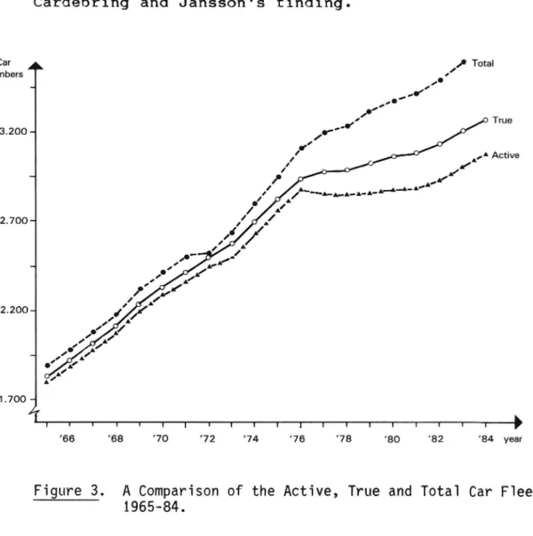
period 1976-84 was only 1.3 per cent. depicts the trend in the active,

fleets since 1965. It can be seen that whereas the active fleet actually fell in 1977 and 1978, this

numbers when

Figure 3

true and total car

apparent decline in car disappears

temporarily passive cars are included. This supports Cardebring and Jansson's finding.

,0 Total Numbers ./ I True 3.200 A, Active 2.700 -2.200 -+ 1.700% I l | l l I | l l l I I l l 1 r f 7 l I 66 68 70 72 74 76 78 '80 '82 '84 year

Figure 3. A Comparison of the Active, True and Total Car Fleets 1965-84.

24

Tabie 5. Anaiysis of the Totai Car Register and Estimated True Car Fieet 1965 84.

YEAR ACTIVE PASSIVE TOTAL ESTIMATED

Temporarily Permanently REGISTERED TRUE CAR

or FLEET Unroadworthy 1965 1,793 30 60 1,883 1,823 1966 1,889 33 57 1,979 1,922 1967 1,976 37 56 2,068 2,013 1968 2,071 38 64 2,173 2,110 1969 2,194 41 76 2,310 2,235 1970 2,288 43 91 2,422 2,331 1971 2,337 46 87 2,489 2,403 1972 2,443 48 18* 2,510 2,492 1973 2,503 76 67 2,646 2,579 1974 2,639 61 91 2,791 2,700 1975 2,760 61 121 2,942 2,821 1976 2,881 65 150 3,096 2,947 1977 2,857 130 208 3,195 2,988 1978 2,856 138 252 3,246 2,995 1979 2,868 170 281 3,319 3,039 1980 2,883 181 312 3,376 3,065 1981 2,893 188 335 3,416 3,082 1982 2,936 203 358 3,497 3,140 1983 3,007 200 386 3,592 3,206 1984 3,081 195 436 3,712 3,276

* A substantiai number of vehicies were administrativeiy deregistered in this year.

25

4. CAR LONGEVITY

4.1 Alternative Forms of Survival Functions

The previous section has described how the age distribution of the true car fleet was derived for the years 1965-1984. Survival functions were then estimated using the variable vintage method. The age-specific scrappage rates q(x) were calculated by

t-l

_ Nt

where qt(x) is the annual scrappage rate for x year old cars in year t, and Ntt_x_l represents the number <1f cars first registered :h1 year t-x-l still in existence at the end of year t.

The proportion of cars surviving to age x was then estimated by

x

Pt(x) = IIO (l qt(x))

(4.2)

Figures 4 anui 5 depict scrappage and survival functions for the period 1965-84, calculated in the» above manner. A feature of the results is that scrappage rates tend to increase to a maximum and then either decline (pre 1980) or stabilise (post 1980). This limits the choice of mathematical form for the survival functions: the exponential functions exhibit

a. constant scrappage rate; the Gompertz, a

continuously increasing one; while the Weibull permits constant, increasing (n: decreasing scrappage rates depending on the parameter values chosen. The logistic function, on the other hand, has the advantage t u : it encompasses age-specific scrappage rates which rise to a maximum. For example, the

26 Scrappage rate 0.4 ~ 0.35 8 0.3 -H X 1965 O / 1970 .25-X .o---".oooooo.. . ' O O _ / II...0' .0'. \ o...'. 0.2 f '.' ...o,- //7 \\'°o.o 0 O a \ 0.15 9 0.1 - 0.05-I I I T I I I I I I I I I I I I I I I I I I 1.7 3.7 5.7 7.7 9.7 11.7 13.7 15.7 17.7 19.7 age

Figure 4. Scrappage Rate Functions 1965, 1970, 1975, 1980 and 1984. Proportion surviving 1.0 ~. . 9. \\ " .Q \ \ "'-.x .0\ 08 \ %.\_{.° \} t a . \ 0'7 _ o. \ a. . o .. \ 0.6 _' I... o a... \ 0.5 . .0 .0 o 0.4 - 1965 0.3 . \\ 0.2 -0.1 '-I l l l I I I I I I I I I I l I I 1 I 1.7 3.7 5.7 7.7 9.7 11.7 13.7 15.7 17.7 19.7 21.7 age

figg:g_5. Surviva] Functions 1965, 1970, 1975, 1980 and 1984.

27

simple two parameter logistic function*:

l

with the consequent scrappage rate function given by log =__ dhif x)

b

=

1

(4.4)

Thus, the scrappage rate saturates at b1. An additional advantage of the two parameter logistic function is that the median life expectancy the age up to which there is a 50 per cent chance of survival - is simply the quotient of the co-efficients.

A variant on this functional form which has been widely used in survival analysis is the three parameter logistic

function:-1

S(x) =

_

(4.5)

with the corresponding scrappage rate

function:-Mx) =

bl

(4.6)

We adopt the common convention of writing the survival proportion P(x) as S(x) when it is taking a specific functional form. For a review of appropriate functional forms, see Elandt Johnson and Johnson (1980).

28

4.2 Estimates of Car Longevity

Both the above functional forms 4.3 and 4.5 were applied to the 1984 data, with the three parameter function exhibiting a slightly better fit. Table 6 presents the results. The survival function was fitted using non-linear estimation techniques, employing the Gauss-Newton Method. A grid of starting values was posited (a = 0.9,1.0; (a) = 4,5,6; C1 = 0.4 0.5, 0.6) and the values a = 1, CO = 6 and C1 =

0.4 were selected. Thereafter, convergence was

achieved in seven iterations. The corrected R2 was 0.9926 anui all the co-efficients were significant at time 1 per cent level. The 1984 co-efficient values were then used as starting values for the estimation of similar functions for the years 1965 to 1983.

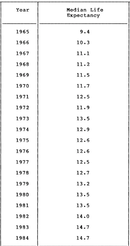
The median life expectancy (MLE) is a convenient way of expressing longevity. Table 7 shows the median life expectancy for the period 1965-84 calculated from the results of Table 6. The estimates can be classified into three periods: from 1965 to 1973, there was a steady increase in MLE, totalling 4 years in all. The year 1972, which provides an exception to

this trend was, in all likelihood, affected by the

change over from local manual to central computerised records which occurred in that year; the second period covers the years 1974 to 1977 when a 1 year

decline in MLE was recorded; in the third period,

from 1978, life expectancy has once again grown steadily, registering a: 2 year increase over the period. The median life expectancy now stands at 14.7 years (1984).

29

Tab1e 6. Estimated 1ogistic surviva1 functions 1965 1984.

Parameter Value Year a C0 C1 N R2 1984 0.9367(0.0181) 3.6832(0.2063) 0.2468(0.0119) 30 0.9926 1983 0.9088(0.0263) 3.2919(0.2513) 0.2197(0.0141) 30 0.9863 1982 0.9350(0.0189) 3.8557(0.2325) 0.2694(0.0142) 30 0.9919 1981 0.9414(0.0220) 3.9395(0.2793) 0.2878(0.0179) 30 0.9893 1980 0.9510(0.0131) 4.3332(0.1953) 0.3180(0.0129) 30 0.9959 1979 0.9612(0.0125) 4.4570(0.1947) 0.3349(0.0132) 30 0.9963 1978 0.9798(0.0060) 5.1736(0.1188) 0.4048(0.0086) 30 0.9990 1977 0.9767(0.0073) 5.6469(0.1709) 0.4479(0.0127) 30 0.9985 1976 0.9779(0.0081) 5.767 (0.1957) 0.4537(0.0144) 30 0.9981 1975 0.9685(0.0116) 5.1748(0.2337) 0.3999(0.0167) 30 0.9963 1974 0.9539(0.0198) 4.6548(0.3340) 0.3539(0.0231) 29 0.9898 1973 0.9633(0.0133) 5.2087(0.2868) 0.3824(0.0200) 17 0.9927 1972 0.9873(0.0039) 5.7932(0.0996) 0.4872(0.0079) 17 0.9994 1971 0.9838(0.0072) 5.7859(0.1993) 0.4606(0.0154) 16 0.9971 1970 0.9826(0.0060) 5.3476(0.1379) 0.4531(0.0111) 16 0.9985 1969 0.9830(0.0076) 5.9362(0.2145) 0.5092(0.0178) 15 0.9971 1968 0.9840(0.0077) 6.0317(0.2344) 0.5332(0.0203) 14 0.9966 1967 0.9833(0.0077) 5.6167(0.2267) 0.5061(0.0204) 13 0.9964 1966 0.9909(0.0045) 6.1063(0.1806) 0.5918(0.0183) 11 0.9981 1965 0.9832(0.0082) 6.6126(0.2617) 0.7100(0.0285) 10 0.9984

Note: Asymptotic standard errors are given in brackets.

30

Perhaps the most interesting feature of Table 7 is the decline in life expectancy which occurred in the post oil crises period 1973-1976. This coincided with an increase in per capita private consumption of 10 per cent over the same period which represents an annual rate of growth some 50 per cent in excess of that for the previous five year period. At the same time new car sales grew substantially to reach an all-time peak of 321,000 units in 1976. It may well be that the additional sales of new cars increased the supply of cars to the used market, thereby depressing used car prices and encouraging scrapping. Although confirmation of this effect must await a fuller analysis of the car market, it is in keeping with the finding of Manski and Goldin (1983) that car scrappage is much more a price related phenomenon than a technical one.

4.3 Comparisons with other Estimates

As mentioned in Section 2.1 above, previous estimates of car longevity in Sweden were undertaken by AB Svensk Bilprovning. These are depicted in Figure 6 together with the estimates made in this study. For years up to 1971, the two sets of estimates are virtually identical. Thereafter, :3 substantial divergence is apparent which by 1982, the latest year for which Bilprovning AB make an estimate, amounts to 2.2 years - a median life expectancy of 16.2 years as compared with 14.0 years as calculated in this study. This difference arises because, for the latter years, the Bilprovning AB estimates are based on total cars, which, as has been shown, includes substantial numbers of permanently passive or unroadworthy cars.

31

Table 7. The revised median life expectancy of cars in Sweden 1965-1984

Year Median Life

Expectancy 1965 9.4 1966 10.3 1967 11.1 1968 11.2 1969 11.5 1970 11.7 1971 12.5 1972 11.9 1973 13.5 1974 12.9 1975 12.6 1976 12.6 1977 12.5 1978 12.7 1979 13.2 1980 13.5 1981 13.5 1982 14.0 1983 14.7 1984 14.7

32

Because the two sources produce almost identical estimates for the pre-l971 period, the analysis of Swedish car MLE can be extended by including AB Svensk Bilprovning estimates for the pre-1965 era (see Figure 6). It is then apparent that the year 1965 represents a turning point in the MLE curve, and the general trend since then has been an upward one.

Mandatory annual vehicle inspection was introduced in Sweden in March 1965 for vehicles of five years 01d and greater. It is possible to view the changes in MLE as arising from this step. The decline in MLE during 1964 and 1965 could be attributed to the scrapping of vehicles in poor condition both in anticipation of inspection and arising from it. This would have weeded out dificient cars and resulted in the short term, in reduced scrapping rates from those remaining. In subsequent years scrappage rates would continue to fall as cars would have higher accumulated maintenance expenditures than their pre-test counterparts, and thus be in better condition. This process would have continued to effect MLE until the number of years, which have elapsed since testing began, exceeded the MLE. For example, in 1979, the MLE was just over 13 years whereas 14 years of inspection had occurred. Thus, a car thirteen years old in 1980 would have accumulated no more annual inspections than its 1979 counterpart, and, ceteris paribus, a reduction in the scrappage rate for this age group could not be expected. MLE would not, therefore, increase. This suggests that, whatever effect the introducthmu of annual vehicle inspection induced, it would have been exhausted by the end of the 19703. Examination of Figure 6 reveals that MLE has continued to grow in the first half of the 19803, and this together with the decrease in MLE in the early 19705, suggests that factors other than annual

Me dian Li fe Exp ec ta nc y me di an lif ee xp ec ta nc y 33 16..A 0/ AB Bilprovning This study I l l I I l l l J F j l. I I F l l V I r T l 1964 1966 1968 1970 1972 1974 1976 1978 1980 1982 1984 Year

Figure 61 Median Life Expectancy 1965-84: A comparison with Estimates made by AB Biiprovning.

AL Sweden 14 -USA 13 12 -11 '10 -9 -1 l I 1 l l I T l I l l l T 71 73 75 77 79 '81 83 year

Figure 7. A Comparison of US and Swedish Median Life Expectancy 1971-1982.

34

vehicle testing have played an important role. Among these are the rate of change in vehicle technology and

conditions in the car market.

As mentioned in Section 2.2 above, a comparison of Swedish car life expectancies with those for other countries is difficult because of the use of different methodologies and data time periods. In order to provide a datum point for comparison with the Swedish results, a study of car survival in the USA was undertaken which provided MLE estimates for the years 1971/72 to 1982/83. More details are given in Appendix 1, where an MLE for 1982/83 of 12.9 years is calculated. Exact year by year comparisons with the Swedish results are not possible, as the USA car fleet is recorded in July of each year, and the Swedish in December. However, Figure 7 partially overcomes this by setting the USA estimates at the mid-year point. Two interesting features emerge. Firstlyy thel USA experience appears to mirror the Swedish but with a lag of approximately 1.5 years: for example, the Swedish downturn of 1973 and upturn of 1978. Secondly, there is a tendency since 1978 for the gap between Swedish and USA values to converge, so that, whereas at the beginning of the period (1971/72) Swedish median car life expectancy was approximately 2 years above the USA value, by 1982/83 this had reduced to just over 1 year.

35

5. CONCLUSIONS

Previous studies have tended to exaggerate car long-evity in Sweden. This has arisen because the method used, namely the comparison of the age distribution of vehicles in the car register in two successive years, assumed that all such vehicles were available for use. However, vehicles may be registered as active or passive and not all passive vehicles return to active use again. For example, this report establishes that for the year 1984, out of a total of 3,712,000 cars in the register, 436,000 must be regarded as permanently passive or scrapped. Thus, the true car fleet, avail-able for use, was 3,276,000, of which 195,000 were temporarily passive vehicles. As previous estimates of car longevity were based on the total register, active p1Us passive, they have been seriously in

error.

The number of passive cars in the register began to grow quickly from about 1973, when the administrative fees for moving a vehicle from active to passive status were abolished and the procedure was also simplified administratively. Thus, relatively speaking, it became easier to make a car passive than to deregister it completely. This has resulted in the inclusion in the register of many unroadworthy vehicles. However, the active car fleet is not a suitable basis for estimating car longevity, either. For many decades, a substantial number of car owners have put their vehicles into passive status for the winter months. As the census of vehicles is undertaken at the end of December each year these wintered vehicles are excluded from the estimated active fleet, even though the majority of them are

36

brought back into active use when weather conditions improve. Cars can be made passive for other reasons, too: if for example, vehicles are undergoing long term repair or are in the process of being sold. This report establishes that a major increase in the number of temporarily passive cars took place in 1977, following a substantial increase in vehicle tax levels and changes ix: the administrative arrangements relating to car dealers' insurance. Because of this growth in temporarily passive cars, the apparent decline in car numbers in 1977 and 1978, as measured by the active fleet, did not, in fact, take place. In the late 19705 and early 19805 the true car fleet has continued to grow, albeit at a much slower rate than in the pre-oil crisis period.

The probability that a car will be made temporarily passive increases sharply with age: less than 4 per cent of cars up to five years of age but more then 25 per cent of those over twenty five years of age are made passive. The domestic Swedish car makes, Volvo and Saab, are considerably less likely to be made temporarily passive.

Using the estimated age distribution of the true car fleet for the period 1965-84, revised estimates of car longevity were made. The median life expectancy of cars was estimated at 14.7 years (1984), which is some 2 years below previous estimates. However, this is still a full five years above the 1965 figure of 9.4 years. Median life expectancy grew strongly in the period to 1973, declined slightly in the post-oil crisis period, and resumed its upward trend in 1978. The strong upward trend in the post-1965 period may be attributed in part to the introduction of mandatory

37

annual vehicle inspection in that year. However, median life expectancy has continued to rise during the early 1980s, when it would be expected that the impact of annual inspection would have fully worked through. It is probable that changes in life expectancy are due to a complicated interaction of changes in vehicle technology, vehicle use, economic conditions and legislative action.

Few studies of median car life expectancy have been conducted for other countries. Those that are available make use of very different measurement methodologies and refer to different time periods and are, therefore, difficult to compare. This study has made estimates of car longevity in the U.S.A. and has shown that for 1982 median car life expectancy is 1 year below the Swedish level. A decade ago, the 'difference was more substantial but there has been a gradual convergence over the period. Another interesting feature is that the USA estimates have tended to mirror the Swedish but with a lag of 1.5 years.

Several implications for statistical policy and further research emerge from this study. Firstly,_it is apparent that neither of the two official measures of the Swedish car fleet accurately reflect the true number of cars available for use on the road. There is a need for Statistiska Centralbyrgn to provide a third and more accurate measure of car numbers on an annual basis. This study presents a methodology for calculating such a series. Secondly, the life expectancy estimates provided by AB Svensk Bilprovning for each make of car are obviously overestimated. The data base developed in this study could be used to recalculate car longevity by make, and in particular, to establish whether certain makes, e.g. Volvo, are

relatively more long-lived than others. Thirdly, there is a need to develop a model of scrapping behaviour which would establish the relative roles played by car age, technology, use levels, economic conditions and legislative actions, such as annual vehicle inspection, in determining car longevity.

39

REFERENCES

1. AB Svensk Bilprovning (1972). The Life Expectancy of Passenger Cars - Calculated in 1972. V311ingby, Sweden.

AB Svensk Bilprovning (1975). The Life Expectancy of Passenger Cars in Sweden -Calculated in 1975. Vallingby, Sweden.

Bennett, T.H. (1976). The Physical Characteristics of the British Motor Vehicle Fleet. The Highway Engineer, Vol. XXIII, No. 10.

Cardebring, Peter och Jan Owen Jansson (1985). Avstéllda bilar cx l Bilstatistiken Meddelande 445; Statens Vag-och Trafikinstitut, Linkoping, Sweden.

Cardebring, Peter (1987). Company and Personal Business Car Ownership Report 305A

ll

Statens Vag-och Trafikinstitut, Linkoping,

Sweden.

Cramer, J.S. (1958). The Depreciation and Mortality of Motor Cars. Journal of the Royal Statistical Society, Series A

(General), Volume 121, Part 1.

Elandt-Johnson, Regina, C. and Norman, L. Johnson (1980). Survival Models and Data Analysis. John Wiley and Sons, New York,

UOSOA.

10. 11. 12. 13. 14. 15. 4O

Ernvall, Timo, (1983). The Service Life of Passenger Cars in Finland. Tie Ja Liikenne,

The Finnish Road Association.

Greene, D.L. and C.K. Eric Chen (1981). Scrappage and Survival Rates of Passenger Car and Light Trucks in the US 1966-77. Transportation Research Vol. 15A, No. 5.

Jansson, Jan Owen, Peter Cardebrimg och Ola Junghard (1986).

Sverige 1950 2010.

Vag-och Trafikinstitut, Linkgping, Sweden.

Personbils-innehavet i

Rapport 301, Statens

Manski, Charles F. and Ephraim Golden (1983). An Econometric Analysis of Automobile Scrappage. Transportation Science Vol. 17, No. 4.

Motor Vehicle Manufacturers' Association of the United States (1985). Facts and Figures 1984. Detroit, Michigan, USA.

Parks, Richard W. (1977). Determinants of Scrapping Rates for Post War Vintage

Automobiles. Econometrica, Vol. 45, No. 5.

SOU (1971). Ett Nytt Bilregister Betankande av Bilregisterutredningen. SOU, 1971:11.

Stockholm,

Kommunikations Departementet,

Sweden.

Thoresen, T. and P. Stella (1977). Analysis of Historical Vehicle Scrapping and Survival Patterns 1950-1976.

Research Forum, Third Annual Meeting.

Australian Transport

41

16. Walker, Franklin V. (1968). Determinants of Auto Scrappage. Review of Economics and Statistics, 52.

42

APPENDIX 1: MEDIAN LIFE EXPECTANCY OF CARS IN THE USA A1.

A2.

*

Introduction

This appendix presents estimates of the median life expectancy of cars in the USA. It is intended to provide evidence with which Swedish results can be compared. The data source was the Motor Vehicle Manufacturers' Association of the United States (1985), which in turn derives the data from R.L. Polk and Co.*. The raw data consisted of the number of cars at July of each year classified by model year.

Methodology and Results

The method used to estimate survival proportions was the variable vintage method.

It was then necessary to associate an exact

age with each survival proportion. July is the observation date for each year, and it can be observed from car registration statistics that typically 65 per cent of cars of a given model year are registered by that date. By linear interpolation, it is possible to estimate that the end of April is the approximate date at which 50 per cent of cars of a given model year have been registered. This gives an age in year t for cars of model year t of 0.225 years.

The authors would like to thank R.L. Polk and Co. for permission to use their data.

Table A1:

43

Survival functions were then estimated for each year using the simple logistic function

l

S(x) = _l+e(bo+le) (A1) This was estimated by non-linear least squares in the manner described in Section 4.2. The results are set out in Table A1 together with the calculated median life expectancy for each year.

Estimated Two Parameter Logistic Survival Functions and Median Life Expectancy for the

U.S.A.

2 Estimated Year Parameter Values N R Medlan L1fe

Expectancy C0 C1 1971/72 5.2119(0.0696) 0.5187(0.0068) 15 0.9995 10.1 1972/73 4.7703(0.0609) 0.4832(0.0060) 15 0.9995 9.9 1973/74 5.2739(0.1146) 0.5061(0.0102) 15 0.9985 10.4 1974/75 5.3350(0.1703) 0.4660(0.0149) 15 0.9961 11.2 1975/76 4.5424(0.1149) 0.4176(0.0105) 15 0.9973 10.9 1976/77 4.4338(0.0778) 0.4251(0.0074) 15 0.9987 10.4 1977/78 4.5003(0.1095) 0.4137(0.0100) 15 0.9974 10.9 1978/79 3.9228(0.1004) 0.3810(0.0096) 15 0.9970 10.3 1979/80 3.9525(0.1048) 0.3848(0.0101) 15 0.9968 10.3 1980/81 4.5008(0.1621) 0.3785(0.0140) 15 0.9934 11.9 1981/82 4.4768(0.1444) 0.3689(0.0123) 15 0.9943 12.1 1982/83 4.9616(0.1978) 0.3860(0.0161) 15 0.9914 12.9