Assessing lidar-based classification schemes for polar stratospheric clouds based on 16 years of measurements at Esrange, Sweden

This is the published version of a paper published in Journal of Geophysical Research: Atmospheres.

Citation for the original published paper (version of record):

Achtert, P., Tesche, M. (2014)

Assessing lidar-based classification schemes for polar stratospheric clouds based on 16 years of

measurements at Esrange, Sweden.

Journal of Geophysical Research: Atmospheres, 119(3): 1386-1405

http://dx.doi.org/10.1002/2013JD020355

Access to the published version may require subscription.

N.B. When citing this work, cite the original published paper.

Permanent link to this version:

RESEARCH ARTICLE

• Recommendations for lidar-based PSC studies

Correspondence to:

P. Achtert, peggy@misu.su.se

Citation:

Achtert, P., and M. Tesche (2014), Assessing lidar-based classifica-tion schemes for polar stratospheric clouds based on 16 years of mea-surements at Esrange, Sweden,

J. Geophys. Res. Atmos., 119, 1386–1405,

doi:10.1002/2013JD020355.

Received 11 JUN 2013 Accepted 7 JAN 2014

Accepted article online 10 JAN 2014 Published online 3 FEB 2014

This is an open access article under the terms of the Creative Commons Attribution-NonCommercial-NoDerivs License, which permits use and dis-tribution in any medium, provided the original work is properly cited, the use is non-commercial and no modifications or adaptations are made.

Assessing lidar-based classification schemes for polar

stratospheric clouds based on 16 years

of measurements at Esrange, Sweden

P. Achtert1_{and M. Tesche}2

1_{Department of Meteorology, Stockholm University, Stockholm, Sweden,}2_{Department of Applied Environmental Science,}

Stockholm University, Stockholm, Sweden

Abstract

classification schemes that apply the backscatter ratio and the particle depolarization ratio. This similarity of input data suggests comparable results of different classification schemes—despite measurements being performed with a variety of mostly custom-made instruments. Based on a time series of 16 years of lidar measurements at Esrange (68°N, 21°E), Sweden, we show that PSC classification differs substantially depending on the applied scheme. The discrepancies result from varying threshold values of lidar-derived parameters used to define certain PSC types. The resulting inconsistencies could impact the understanding of long-term PSC observations documented in the literature. We identify two out of seven considered classification schemes that are most likely to give reliable results and should be used in future lidar-based studies. Using polarized backscatter ratios gives the advantage of increased contrast for observations of weakly backscattering and weakly depolarizing particles. Improved confidence in PSC classification can be achieved by a more comprehensive consideration of the effect of measurement uncertainties. The particle depolarization ratio is the key to a reliable identification of different PSC types. Hence, detailed information on the calibration of the polarization-sensitive measurement channels should be provided to assess the findings of a study. Presently, most PSC measurements with lidar are performed at 532 nm only. The information from additional polarization-sensitive measurements in the near infrared could lead to an improved PSC classification. Coincident lidar-based temperature measurements at PSC level might provide useful information for an assessment of PSC classification.

1. Introduction

The majority of observations of polar stratospheric clouds (PSCs)—especially long time series—are based on lidar measurements of their optical properties [David et al., 1998; Santacesaria et al., 2001; Adriani et al., 2004; Blum et al., 2005; Massoli et al., 2006]. Consequently, PSC properties are generally related to the opti-cal effects they were inferred from. These effects are (1) the strength of the return signal of a PSC and (2) the influence of a PSC on the state of polarization of the linearly polarized laser light. Our knowledge of PSCs is strongly linked to the development of the measurement capabilities of the applied instruments and has improved as lidars have become more advanced, precise, and widespread. While it is straightforward to identify the occurrence and exact location of a PSC in a lidar measurement, it is complicated to derive details about its microphysical properties. The connection between a lidar measurement of a PSC and the alloca-tion of certain microphysical properties based on the informaalloca-tion obtained from the measurement is what will be referred to as PSC classification in this paper.

Poole and McCormick [1988] (P88 from here on) presented the first lidar-based classification of Antarctic

PSCs. The authors could separate two types of PSCs from the lidar measurements. Type I showed a small

total backscatter ratio (ratio of total to molecular backscatter coefficient, R_T< 5) and a low particle

depolar-ization ratio (𝛿_par < 5%). Type II PSCs showed a strong increase in both the total backscatter ratio (R_T > 5)

and the particle depolarization ratio (𝛿par > 20%) that is typical for nonspherical ice crystals. The findings

were in accordance with the theoretical understanding of PSC formation at that time [McCormick et al., 1985;

Toon et al., 1986; Crutzen and Arnold, 1986].

In the following two decades, lidar-based PSC classification evolved from the first two-type separation to very detailed schemes that rank up to six different types and subtypes of PSCs. These classification schemes

were developed based on the observed occurrence rate of the combination of optical parameters (e.g.,

RTversus𝛿par). The identified clusters were then related to microphysical properties (size distribution and

shape) of the scatterers through the findings of light-scattering calculations with spherical and nonspherical particles [Biele et al., 2000; Pitts et al., 2009, 2013].

The evolution of classification schemes implies that different studies in the literature have been based on different classification schemes. Note that the latter were usually developed to suit the observations per-formed with a particular instrument and might account for known calibration errors and measurement uncertainties that are not explicitly mentioned in the respective publications. Consequently, different research groups tend to prefer different classification schemes, and the literature on PSC observations always needs to be put into the context of which scheme was applied. This circumstance calls for an inves-tigation of the comparability of the different classification schemes when applied to the measurement of a single instrument.

This paper presents a comparison of different classification schemes used for long-term analysis of PSCs observed by ground-based lidar systems over Antarctica [Santacesaria et al., 2001; Adriani et al., 2004] and the Arctic [Blum et al., 2005; Massoli et al., 2006] as well as with the spaceborne Cloud-Aerosol Lidar and Infrared Pathfinder Satellite Observations (CALIPSO) lidar [Pitts et al., 2007, 2009, 2011, 2013]. The classifi-cation scheme of Massoli et al. [2006] that will be discussed in detail in this paper is based on Adriani et al., [2004]. The ground-based schemes include three different types of PSCs which were first proposed by

Browell et al. [1990] and Toon et al. [1990]. Type I was split into two subclasses. Type Ia showed small

backscatter ratios and large particle depolarization ratios typical for solid nonspherical particles. Type Ib showed large backscatter ratios and low particle depolarization ratios typical for liquid particles. From these and earlier lidar observations of PSC optical properties it was inferred that type Ia consists of nitric acid tri-hydrate crystals (NAT) while type Ib is made up of supercooled liquid ternary solutions (STS) that consist of

H2SO4, HNO3, and H2O and occur at temperatures below 195 K [Peter, 1997]. Type II PSCs were found to be

formed below the ice-frost point and to consist of water-ice crystals [McCormick et al., 1982, P88]. In contrast to the liquid STS droplets and the small NAT particles, ice crystals have a strongly nonspherical shape and cover a size range that is very efficient in interacting with light at visible wavelengths [Sassen, 2005]. Conse-quently, their optical effects are quite different from the ones of STS and NAT particles. Ice crystals can easily be identified in a lidar signal since they have a significant effect on the state of polarization of the scattered laser light. This effect is measured as depolarization ratio. There is a difference between the total volume depolarization ratio (molecules and particles) and the particle depolarization ratio, and many publications miss to properly state which parameter is used in the specific study. Depolarization-ratio measurements require both well-characterized instruments and calibration routines [Biele et al., 2000; Reichardt et al., 2003;

Alvarez et al., 2006; Freudenthaler et al., 2009].

In addition to the three traditional PSC types several subtypes of PSC with low to moderate backscatter ratios and moderate to high particle depolarization ratios have been described in the literature. All sub-types, e.g., type Ia enhanced [Tsias et al., 1999], type Ic [Tabazadeh and Toon, 1996; Toon et al., 2000], type Id [Stein et al., 1999], NAT rocks [e.g., Fahey et al., 2001; Brooks et al., 2003], or intermediate PSCs with lidar sig-nals ranging between those typical for type Ia and type Ib [David et al., 2005], are expected to consist of the same constituents as the main types but show different scattering characteristics.

Since January 1997 a Rayleigh/Raman lidar has been operated at Esrange (68◦N, 21◦E) in northern Sweden,

about 150 km north of the Arctic circle. This lidar is well equipped for the observation and classification of PSCs [Blum et al., 2006; Khosrawi et al., 2011; Achtert et al., 2011]. In this study we present a comprehensive data set of PSC observations, classify the observed clouds according to commonly used lidar-based PSC classification schemes, and perform a statistical analysis on the rate of occurrence of the different cloud types and subtypes in the respective schemes.

We begin this paper with a brief description of the Esrange lidar and its 16 year PSC data set in section 2. Section 3 introduces the optical properties used for lidar-based PSC classification, puts them into relation to the microphysical properties of PSC particles, and gives a brief review of the PSC classification schemes available in the literature. The results of applying the different schemes to the Esrange lidar data set are presented in section 4. The study ends with a discussion of our findings in section 5 and our conclusions in section 6.

2. Esrange Lidar and the PSC Data Set

The Department of Meteorology of the Stockholm University operates the Esrange lidar at Esrange (68◦N,

21◦E) near the Swedish city of Kiruna [Blum and Fricke, 2005; Achtert et al., 2013]. It was originally installed

in 1997 by the University of Bonn. The Esrange lidar uses a pulsed Nd:YAG solid-state laser as light source. A detection range gate of 1 μs results in a vertical resolution of 150 m. The backscattered light at 532 nm is detected in two orthogonal planes of polarization. Light with the same plane of polarization as the

emitted laser light is referred to as parallel polarized or co-polarized (superscript‖), and light with a

polar-ization plane perpendicular to the one of the emitted laser light is called perpendicularly polarized or

cross-polarized (superscript⊥).

Measurements of backscattered light in the parallel and perpendicular channels are used to derive the

par-allel and perpendicular backscatter ratios (R‖and R⊥, respectively), the particle backscatter coefficient (𝛽par),

and the linear particle depolarization ratio (𝛿par) assuming molecular scattering characteristics. In contrast to

the volume depolarization ratio (𝛿vol) that was used in the first PSC studies, the particle depolarization ratio

contains no contribution of molecular scattering. Depolarization-ratio measurements with the Esrange lidar [Blum et al., 2005] are calibrated according to the method described by Biele et al. [2000]. Additional calibra-tion measurements using white light with a controlled state of polarizacalibra-tion [Mattis et al., 2009] revealed that the cross talk between the polarized channels and polarizing effects of the receiver optics of the Esrange lidar are negligible.

The molecular fraction of the received signal is determined either from the vibrational Raman signal or by use of a concurrent ECMWF (European Centre for Medium-Range Weather Forecasts) temperature and pres-sure analysis. The lidar signal (aerosols + molecules) is normalized to the molecular signal in the aerosol-free part of the atmosphere for the calculation of the backscatter ratios. According to the spectral range of the

interference filters in the detector, the value of the molecular depolarization ratio is assumed as𝛿mol =

0.36% [Blum and Fricke, 2005]. Since 2011 the Esrange lidar is equipped with rotational-Raman channels for temperature profiling in the troposphere and lower stratosphere. General details about the instruments are provided in Blum and Fricke [2005] and Achtert et al. [2013].

In addition to basic scientific studies, the lidar has developed into an important tool to support balloon, air-craft, and rocket campaigns based at Esrange. PSC measurements with the Esrange lidar during the time period 1997–2005 including a statistical analysis have been presented by Blum et al. [2005]. Since then seven more years were added to the time series that now covers 16 years or 542 h of PSC observation. Note that the measurements were conducted on campaign bases during northern-hemispheric winter and that there were several winters during which few or no PSCs were observed over Esrange due to early major stratospheric warmings. The Esrange lidar PSC data set contains hourly mean values of the parallel and per-pendicular backscatter ratio and the particle depolarization ratio with a vertical resolution of 150 m—all measured at 532 nm. It forms the foundation of the investigation of the performance of the different PSC classification schemes discussed in this study.

3. PSC Classification With Lidar

This section provides an overview of the parameters that are typically used for PSC classification. It also pro-vides a review of PSC classification schemes that are commonly used in the literature. Note that different

classification schemes rely on different parameters (e.g.,𝛿_parversus R_Tor𝛿_parversus R‖) and that it is not

always clear from the literature which parameter is actually used. In order to avoid further ambiguity, we also want to clarify the differences between the parameters used.

3.1. Optical Parameters Used for PSC Detection

Since the late 1980s PSCs are routinely monitored by ground-based lidar systems in Antarctica [e.g., Iwasaka

and Hayashi, 1991; Stefanutti et al., 1991] and since the beginning of the 1990s in the Arctic [e.g., Krüger,

1994; Toon et al., 1990; Schäfer et al., 1994; Beyerle et al., 1997]. The primary variables determined for PSC

detection are the backscatter ratio R and the linear particle depolarization ratio𝛿par. The general definition

of the backscatter ratio is

R = 𝛽 𝛽mol

= 𝛽par+𝛽mol

𝛽mol

where the total volume backscatter coefficient𝛽 represents the sum of the particle backscatter coefficient

𝛽parand the molecular backscatter coefficient𝛽mol. The backscatter ratio allows for a straightforward

esti-mation of the contribution of non-Rayleigh scattering in the atmosphere, since𝛽_molcan be easily derived

from a standard atmospheric model or a nearby radiosonde ascent [Bucholtz, 1995]. The backscatter ratio is unity for a pure Rayleigh atmosphere and increases with increasing contribution of nonmolecular scat-terers in the air. Note that the definition in equation (1) is only true for lidar systems that measure a total backscattered signal, i.e., a signal that does not refer to a certain state of polarization of the backscattered light. If backscattered light is measured in separate channels for the detection of light that is polarized par-allel and perpendicular with respect to the plane of polarization of the emitted linearly polarized laser light,

the definition of𝛽 changes to

𝛽T=𝛽par‖ +𝛽 ⊥ par+𝛽 ‖ mol+𝛽 ⊥ mol. (2)

Now𝛽‖parand𝛽par⊥ represent the co- and cross-polarized backscatter coefficient, respectively. To avoid

misunderstandings, the total particle backscatter coefficient that is derived from polarization-sensitive

mea-surements will be called𝛽Tin this study. Combining equations (1) and (2) leads to the total backscatter ratio

for polarization-sensitive measurements

RT= 𝛽‖ par+𝛽par⊥ +𝛽 ‖ mol+𝛽mol⊥ 𝛽‖ mol+𝛽 ⊥ mol . (3)

The backscatter ratio can also be calculated individually from the measurements in the polarized channels as R‖=𝛽 ‖ par+𝛽‖mol 𝛽mol‖ (4) and R⊥=𝛽 ⊥ par+𝛽⊥mol 𝛽⊥ mol . (5)

The linear particle depolarization ratio is derived from the measurements of cross- and co-polarized signals as 𝛿par= 𝛽⊥ par 𝛽par‖ = ( R⊥− 1 R‖− 1 ) 𝛿mol, (6)

where𝛿mol=𝛽mol⊥ ∕𝛽

‖

molis the molecular depolarization given as the ratio of perpendicular to parallel

molec-ular backscatter coefficient. The molecmolec-ular depolarization ratio is constant with height and depends on the

optical elements in the lidar receiver. It is𝛿mol = 0.36% in the case of the Esrange lidar [Blum and Fricke,

2005]. It should be noted that polarization-sensitive measurements require well-characterized instruments and reliable calibration routines since even slight amounts of cross talk between the co- and cross-polarized channels (i.e., few percent of parallel polarized light in the perpendicular channel) can introduce significant uncertainty to the measured particle depolarization ratio [Mattis et al., 2009].

To be able to properly compare the classification schemes that were developed for very different lidar sys-tems, we have to assume that instrumental effects are negligible. Such effects (e.g., insufficiently clean polarization of the emitted laser light, system misalignment, bad background suppression, background signal estimation, assumptions used for the inversion method, cross talk in the polarized channels, or depo-larization effects of the receiver optics) should be included in the systematic and methodological error of the studies available in the literature. Otherwise, a PSC classification scheme that has been developed based on measurements of a lidar system that suffered from significant instrumental effects (known or unknown) is likely to be adapted to account for these effects. Note that the information on measurement errors that is necessary to assess the quality of the classification scheme is rarely given in the respective literature. The influence of the measurement error of the Esrange lidar on PSC classification will be discussed in detail in section 4.4.

Table 1. PSC Classification Related to Optical (Measured by Lidar) and Microphysical Propertiesa

Likely Microphysical Typical Particle

PSC Type R‖ R⊥ _𝛿par(%) Composition Radius

None low low low Binary H₂SO₄−H₂O ≈0.1μm

(background) droplets

Ia low low-medium large few solid hydrates 1–10μm

HNO₃–3H₂O or HNO₃–2H₂O

Ia enhanced low medium-large medium-large predominantly solid ≈0.3μm hydrates

Ib low-medium low low Ternary ≈0.3μm

HNO₃−H₂SO₄–H₂O

II large very large medium-large ice crystals _≥1.5μm

a_{The table is adapted from B01. Signals with a low, medium, and large intensity correspond to backscatter}

ratios (particle depolarization ratios) of<5 (<5%),<10 (<10%), and>10 (>10%), respectively.

3.2. Connection of Lidar Optical Parameters to PSC Microphysical Properties

The optical properties detected with lidar are related to the microphysical properties of the scatterers in the instrument’s field of view. However, it is hard to draw more than qualitative conclusions from the parameters that are obtained from a lidar measurement. The backscatter ratio is an extensive property that depends on the size distribution of the scattering particles in a volume, including total volume concentration. It is used to investigate how far an observation deviates from the particle-free background conditions. Consequently, low and high backscatter ratios mark low and high particle concentrations, respectively. Reichardt et al. [2002] showed that the backscatter coefficient and the backscatter ratio cannot be used for an inversion of lidar data that would give information on the microphysical properties of a PSC. Preferably, intensive optical properties that depend on the type of scatterer rather than its concentration should be used for this pur-pose. Such properties are the color ratio (ratio of the backscatter coefficients at two wavelengths), the lidar ratio (ratio of the extinction and the backscatter coefficient), and the particle depolarization ratio. Spherical scatterers like STS droplets do not influence the state of polarization of scattered light [Peter, 1997]. Conse-quently, the particle depolarization ratio is close to zero for clouds that contain a large volume fraction of liquid droplets. Nonspherical particles like NAT particles and ice crystals on the other hand can depolarize the incoming laser light during the scattering process. This leads to nonzero signals in the perpendicular channel and increased particle depolarization ratios. The interpretation of two coexisting particle classes (spherical and nonspherical) can be improved if the backscatter coefficients or backscatter ratios are studied separately for both states of polarizations [Biele et al., 2001; Reichardt et al., 2004]. Irregularly shaped ice

crys-tals are known to produce the highest values of𝛿parwhich is why they can easily be identified in the lidar

measurement [Sassen and Benson, 2001].

Table 1 gives an overview of how optical properties can be related to microphysical properties. Note that

there is no simple relationship between𝛿_parand particle shape [Liu and Mishchenko, 2001; Reichardt et al.,

2002]. Reichardt et al. [2004] showed that especially for solid particles a variety of shapes are consistent with similar lidar observations. Spheroids or cylinders are commonly used for the interpretation of lidar mea-surements of type Ia PSCs [Toon et al., 2000; Liu and Mishchenko, 2001; Brooks et al., 2004; Pitts et al., 2009;

Lambert et al., 2012]. Reichardt et al. [2004] compared lidar data obtained with two lidar systems at Esrange

to the optical properties derived from scattering calculations with spheroids, hexagons, and irregularly shaped particles. Measurements of NAT particles showed good agreement with simulations for irregu-lar particles with an aspect ratio between 0.75 and 1.25, maximum dimensions from 0.7 to 0.9 μm, and a

number density from 7 to 11 cm−3_{. Further, Reichardt et al. [2004] showed that lidar observations at longer}

wavelength—preferably the particle depolarization ratio, backscatter ratio, and lidar ratio at 1064 nm—are needed for a more accurate size estimation of large NAT particles and ice crystals. Observations at longer wavelengths are more sensitive to the occurrence of few large nonspherical scatterers in the presence of numerous STS particles [Toon et al., 2000; Brooks et al., 2004]. Relying only on measurements of the particle depolarization ratio in the visible can cause incorrect identification of mixed clouds (STS + NAT) as solution droplets (STS).

During the last 17 years several stratospheric balloons were launched from Esrange to study the particle number size distribution, the chemical composition, and the optical properties of PSCs in connection with lidar measurements. Schreiner et al. [2003] showed that the backscatter ratio, the depolarization ratio, and the particle size distribution of a PSC observed in January 2000 are strongly correlated to measurements performed with an aerosol composition mass spectrometer. Voigt et al. [2003] used a particle size distribu-tion from a balloon-borne in situ measurement as input to an optical model to calculate backscatter ratios at different wavelength for comparison with a concurrent lidar measurement of a mountain-wave PSC.

The latter was found to mainly consist of NAT particles with number densities between 0.01 and 0.2 cm−3_,

median particle radii of 1 to 2 μm, and volume concentrations of up to 1 μm3_cm−3_{. A good agreement}

between the measurements and the optical simulations was achieved using aspherical NAT particles with an aspect ratio of 0.5. The median radius of the NAT particle size distribution measured by Schreiner et al.

[2003] was between 0.5 and 0.75 μm at concentrations around 0.5 cm−3_{. Deshler et al. [2003] showed that}

balloon-borne in situ measurements of three distinct PSC layers between 22 and 26 km performed on 9 December 2001 were in agreement with ground-based lidar observation at Esrange. In the lower layer the particles were primarily composed of STS, while the middle layer consisted of NAT particles. A low concen-tration of large, solid particles containing significant amounts of water and nitric acid was measured in the cloud layer. An embedded thin ice layer was observed in the STS layer during the first ascent of the balloon. The ice layer showed a rapid increase in the volume depolarization ratio (measured by laser backscatter-sonde), particle water mass, and particle radius. In addition, the backscatter ratio was more than twice as high as in the NAT layer [Deshler et al., 2003].

3.3. PSC Classification Schemes

PSCs are classified according to their scattering characteristics using the lidar-based variables R_T, R‖, R⊥,

and𝛿par. Table 2 gives an overview of the thresholds of the parameters that are used to identify different

PSC types in commonly used classification schemes. The classification schemes were developed for dif-ferent lidar systems (ground-based, airborne, and spaceborne) and different geographical locations. Note that in case of lidars with well-constrained measurement errors there is no reason why the definition of the thresholds should vary significantly depending on the location.

The earliest classification schemes by Browell et al. [1990] and Toon et al. [1990] (B90 and T90, respectively,

from here on) separated the three traditional PSC types (Ia, Ib, and II) from measurements of RTand𝛿parat

wavelengths of 603 and 1064 nm, respectively (Table 2). These measurements were conducted with the NASA Langley Research Center’s airborne differential absorption lidar flown on the NASA Ames Research Center’s DC-8 aircraft during the Arctic polar winter 1988–1989. The backscatter ratio used in these studies was defined according to equation (1). However, measurements were conducted for separated parallel and perpendicular signals.

Stein et al. [1999] (S99 from here on) used thresholds based on B90 and T90 for the three traditional PSC

types but for lidar measurements at 532 nm performed at Sodankylä, northern Finland, during two win-ter campaigns in 1994/1995 and 1996/1997. The observed total backscatwin-ter ratios for types Ia and Ib were in good agreement with the values reported in the previous publications. However, the observed particle depolarization ratios for type Ia PSCs were found to be between 5% and 25%. This is rather low compared to the previous observation by B90 and T90 with values between 30 and 50%. Furthermore, S99 identi-fied a third class of type I PSCs which they named type Id. This PSC type showed larger total backscatter

ratios (RT < 3) than type Ia PSCs (RT < 1.5, Table 2) and was assumed to contain coexisting solid and

liquid particles.

Santacesaria et al. [2001] (S01 from here on) published a PSC climatology based on lidar measurements at

Dumont d’Urville, Antarctica, between 1989 and 1997. PSC observations are arranged in a𝛿par-versus-RT

space. The climatology presented by S01 is a continuation of an earlier PSC climatology for the years from 1989 to 1993 [David et al., 1998]. The lidar system at Dumont d’Urville measured both planes of polarization at 532 nm, and the backscatter ratio was defined as in equation (1). The particle depolarization ratio used in S01 was not defined as in equation (6) but as the ratio of cross-to-total backscatter coefficients

𝛿′ par= 𝛽⊥ par 𝛽⊥ par+𝛽 ‖ par = 𝛿par 1 +𝛿par . (7)

Ta b le 2 . T h re shold V alues o f R and 𝛿par U sed fo r the S e lec tion of PSC Type in C ur re nt Classification S chemes A v ailable in the L it eratur e a Ia NA T subt ype Ib II M IX Backg round RR 𝛿par (%) R 𝛿par (%) R 𝛿par (%) R 𝛿par (%) R 𝛿par (%) R P oole a nd McC o rmick [1988] P 88 ‖ not classified not classified not classified > 5 > 20 < 5 < 5 < 1.1 Bro w ell et a l. [1990] B 90 T 1.20–1.50 30.0–50.0 not classified 3.00–8.00 0.5–2.5 > 10.0 > 10.0 not classified ≤ 1.20 Toon et al .[1990] T 90 T 2.00–5.00 30.0–50.0 not classified 5.00–20.00 < 4.0 > 2.0 > 10.0 not classified ≤ 2.00 Stein et a l. [1999] S 99 T 1.10–1.50 < 25.0 1.10–3.00 < 15.0 < 8.00 0.3–2.5 not classified Biele et a l. [2001] b B01 ‖ < 1.20 1.50–7.00 > 1.18 > 7.0 1.18–7.00 c < 1.18 ⊥> 1.31 > 1 + 55 ( R ‖− 1 ) d < 1.31 > 85.0 < 1 + 55 ( R ‖− 1 ) < 1.31 > 1.31 S a ntac esaria et al .[2001] e S01 T < 2.00 < 100 2.00–6.00 > 25.0 2.00–5.00 < 2.6 > 10.0 > 9.9 < 10.00 c 2.6–11.1 A driani et a l. [2004] A04 T 1.10–1.56 > 10.0 1.56–5.00 20.0–35.0 > 1.43 < 3.0 < 10.0 > 30.0 < 1.43 c < 10.0 < 1.10 1.43–1.56 f 3.0–10.0 1.56–10.00 f 3.0–20.0 5.00–10.00 g > 20.0 Blum et al .[2005] B 05 ‖ 1.06–2.00 > 10.0 not classified 1.06–5.00 < 0.7 2.0–7.0 > 2.0 remaining p oints < 1.06 > 7.0 Massoli et al .[2006] M 06 T 1.15–1.56 > 10.0 1.56–5.00 > 20.0 > 1.43 < 3.0 > 10.0 > 30.0 < 1.45 < 10.0 < 1.15 1.43–1.56 3.0–10.0 1.56–10.00 3.0–20.0 P itts et al .[2009] h P09 T not classified 2.00–5.00 > 10.0 > 1.25 0.5–3.5 > 5.0 0.5 − 2.0 1.25–5.00 3.0–36.0 1.32–2.60 i P itts et al .[2011] P 11 > 50.0 1 − 0.5 < 1.1 > 3.5 1.32–2.60 g aAll o bser vations w er e p er fo rmed at 532 nm, ex ce pt fo r B 90 and T 90 who u sed 603 and 1064 nm, re spec tiv e ly .T he thir d column denot e s the applied co mponent of the b ackscatt er ratio: to tal (T ), parallel ( ‖ ), or per p endicular ( ⊥ ). Not e that not a ll classification schemes inc o rp orat e the same PSC types .N A T subt ypes includes ty pe Ia enhanc ed .T ype Ia enhanc ed is classified in B01 ,S 01, A04, and M 06. bP a rt icle depolarization ratios ar e deriv ed fr om the combination of the co -and cr oss-polariz e d b ackscatt er ratios; re scale for diff e re nt re lativ e e rr or . cM ix tur e o f type Ib a nd ty pe II PSC p ar ticles . dC o rr esponds to a m inimum aer osol depolarization of 𝛿par = 20 % for nonspherical par ticles p re sent; 55 = 0. 2 ∕ 0. 0036 ;r escale fo r lidar sy st ems with other values o f m olecular depolarization. eV a lues o f 𝛿 ′ par fr om S01 w er e transf o rmed to 𝛿par as descr ibed in equation (7). fM ix tur e o f type Ia a nd ty pe Ib PSC p ar ticles (MIX A ). gM ix tur e o f type Ia enhanc ed and type II P SC par ticles (MIX B ). hIn addition, n onspher ical par ticles a re identified thr ough nonz er o v alues o f the per p endicular b ackscatt er co efficient e v e n in cases of backscatt e r ratios at backg round lev e l. iVa lues depend on the h oriz ontal a v e rage used in the a naly sis .A v alue of 1.1 was u sed in this study to ac co unt for g round-based lidar data being less n ois y than spac e borne o bser va tions .

The thresholds chosen for the three traditional PSC types described in S01 are similar to B90, T90, and S99.

However, since S01 use𝛿′

parthese thresholds are actually slightly higher compared to the previous

stud-ies when transformed to𝛿_paraccording to equation (7). In Table 2 the original thresholds of𝛿′

parfrom S01

were converted to𝛿_parfor better comparability. As in S99, S01 observed an additional class of type I PSCs

that showed increased values of R_Tand𝛿_par. This observation cannot be explained by a mixture of different

particle types. It is more likely to represent NAT particles which formed closer to thermodynamic equilib-rium as compared to the typical type Ia particles. Consequently, this type is referred to as type Ia enhanced

[Tsias et al. 1999; S01]. Furthermore, S01 introduced another class with RT< 10 and 𝛿parbetween 2.5% and

10%. According to the authors, the latter class represents a mixture of type Ib liquid droplets and type II water-ice particles.

Adriani et al. [2004] (A04 from here on) published a PSC climatology derived from lidar measurements over

McMurdo Station, Antarctica, between 1993 and 2001. Their lidar measured signals in two planes of polar-ization at 532 nm. The backscatter ratio was defined as in equation (1) and the particle depolarpolar-ization ratio as in equation (6). The chosen thresholds of R for the three traditional PSC types are similar to B90 and T90 (see Table 2). The lower thresholds of the particle depolarization ratio are 10% and 30% for PSCs of type Ia and II, respectively, rather than 30% and 10% as defined by B90 and T90. The conservative approach in clas-sifying ice PSCs (i.e., the high threshold value of the particle depolarization) is due to the notion that the particle depolarization ratio of PSC ice is expected to be in the range of values observed for cirrus clouds [Sassen and Benson, 2001]. The classification scheme also includes type Ia enhanced with a lower backscat-ter ratio than defined in S01 but similar values as the type Id of S99. Furthermore, A04 introduced two mixed-cloud classes: MIX A represents a mixture of type Ia solid particles and Ib liquid droplets, and MIX B describes a mixture of type Ia enhanced particles and type II water-ice crystals.

A PSC climatology derived from lidar measurements at Ny Ålesund, Spitsbergen, that spans over the winters from 1995/1996 to 2003/2004 was published by Massoli et al. [2006] (M06 from here on). The lidar system at Ny Ålesund also measured backscattered light at 532 nm in two orthogonal planes of polarization. The total backscatter ratio was defined as in equation (1) and the particle depolarization ratio as in equation (6). M06 used the same thresholds as A04 for the three traditional PSC types and the additional subtypes. However, the classification scheme of M06 does not feature the MIX B class of A04. The distribution of data points are

arranged in a𝛿par-versus-(1 − 1∕RT) space.

A detection and classification algorithm for PSC measurements with the spaceborne CALIPSO lidar (oper-ational since June 2006) was developed and refined by Pitts et al. [2007], Pitts et al. [2009], and Pitts et al. [2011], respectively (P09 and P11 from here on). This scheme largely adopted the classification presented

in A04 and M06. The PSC observations are classified in a𝛿par-versus-1∕RTspace. P09 again defined new

composition classes. Instead of type Ia they introduced another two different MIX classes based on model calculations for mixtures of STS and NAT particles with different concentrations. MIX 1 and MIX 2 are

mix-tures of type Ia and type Ib PSCs with lower or higher NAT number density/volume than NNAT= 10−3cm−3,

respectively, and a total backscatter ratio RT < 1.25. In accordance to the NAT subtypes of previous

schemes, MIX 2-enhanced was introduced later by P11 and is defined as RT > 2 and 𝛿par > 10%. PSCs of

type Ib have a threshold of𝛿par < 3.5% for 1.25 < RT < 2.5 which then linearly decreases to 𝛿par < 3%

at RT = 3.3 followed by a further linear decrease to 𝛿par < 0.5% at RT > 100. P09/P11 is applied to rather

noisy CALIPSO level 1 data, and features with negative particle depolarization ratios as low as𝛿par = −10%

are classified as type Ib PSCs. Type II PSCs show values of RT > 5 with 𝛿parbetween 0.5% and 2.0%. Type II

PSCs with very high backscatter ratios of RT> 50 are interpreted as being formed by mountain waves. Note

that the signal-to-noise ratio (SNR) of the PSC observations with CALIPSO depends on the applied horizontal averaging range (5, 15, 45, or 135 km) and that the background threshold value decreases with increasing SNR. Because the SNR of ground-based lidar measurements is much lower than what can be expected from

spaceborne observations, we applied a background value of RT = 1.1 when applying the P09/P11 scheme

to observations of the Esrange lidar.

The lidar-based PSC classification schemes discussed so far apply a combination of the particle depo-larization ratio and either the total backscatter ratio or the backscatter ratio measured in one plane of polarization. In contrast to that, Biele et al. [2001] and Blum et al. [2005] introduced classification schemes which apply the co- and cross-polarized backscatter ratios at 532 nm. Biele et al. [2001] (B01 from here on) analyzed PSC measurements performed at Ny Ålesund between 1995 and 1997. They concluded

Figure 1. Picture of an ice PSC (mother-of-pearl cloud) observed over Esrange in the afternoon of 27 January 2011. Picture taken by the authors.

that the polarized backscatter ratios are more sensitive indicators for the presence of nonspherical solid particles than the particle depolarization ratio. The classification scheme developed by B01 includes PSCs of type Ia, type Ia enhanced, type Ib, and type II (see Table 2). The type Ib PSC class was divided into a pure liquid-phase type Ib and a mixed-phase type Ib. The mixed-phase type Ib PSCs refer to a presence of solid particles. The choice of the actual thresholds of the co- and cross-polarized backscatter ratios in B01

depends on the relative error of the measured R‖and R⊥. Typical values of the relative error (including

ran-dom and systematic error) of the measurements conducted by B01 are 10% for the parallel and 18% for the perpendicularly polarized backscatter ratio. Furthermore, the lidar observations were compared with opti-cal simulations. Typiopti-cal values of the relative error of the Esrange lidar are 9.2% for the parallel and 15.5% for the perpendicularly polarized backscatter ratio. In Table 2 the criteria for the different classes are calculated according to the relative error of the Esrange lidar. Table 1 shows a PSC classification scheme according to B01 relating optical properties measured by lidar to the microphysical properties of PSCs. Note that none of the previously discussed classification schemes includes measurement uncertainties in the selection of PSC types.

Blum et al. [2005] (B05 from here on) published a PSC climatology based on lidar measurements at Esrange

during the winters from 1996/1997 to 2003/2004. Their classification scheme is based on B90 and features

the three traditional PSC types Ia, Ib, and II. The PSC observations are arranged in a R‖-versus-R⊥space. Type

Ia PSCs are identified by low parallel backscatter ratios (R‖ < 2.0) and large particle depolarization ratios

(𝛿par > 10.0%). Type Ib PSCs show large parallel backscatter ratios (up to R‖ = 5.0) and very small particle

depolarization ratios (𝛿_par< 0.7%). Type II PSCs are represented by large backscatter ratios in both

polariza-tion planes (R‖> 2.0 and R⊥> 7.0) and particle depolarization ratios of 𝛿_par> 2.0%. Observations which do

not meet the criteria for the three classes are classified as MIX (see Table 2).

4. Results

Before applying the classification schemes reviewed in section 3.3 to the 16 year Esrange lidar data set, we will present the results for two individual cases: an ice PSC observed on 27 January 2011 and a non-ice PSC observed on 8 January 2012. These two cases are used to assess how well ice and non-ice PSCs are handled by the different schemes.

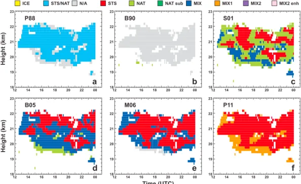
Figure 2. Classification of a PSC observed over Esrange between 1430 and 1900 UTC on 27 January 2011 according to six different schemes: (a) P88, (b) B90, (c) S01, (d) B05, (e) M06, and (f ) P11. Colors refer to different constituents: water ice (yellow), a mixture of NAT and STS (light blue, only for P88), not classified (gray), STS (red), NAT (light green), NAT subtypes (dark green, only in S01 and M06), mixtures (dark blue, only in S01, B05, and M06), and the different mixtures resolved only by P11. Note that the combination of MIX 1 and MIX 2 is comparable to the MIX class of other schemes and that MIX 2 enhanced is similar to the NAT subtypes. Missing pixels in individual displays denote bad data (in contrast to not classified). The photo in Figure 1 suggests that this PSC consisted mainly of water-ice crystals.

4.1. Case of an Ice PSC Observed on 27 January 2011

An ice PSC was observed with the Esrange lidar between 1430 and 1900 UTC on 27 January 2011. The cloud showed a colorful mother-of-pearl appearance (Figure 1) that is a clear sign for the presence of ice particles [Hesstvedt, 1962]. On this day the southern edge of the polar vortex was located over northern Scandinavia. Vertically propagating mountain waves were generated at the Scandinavian mountain range. Stratospheric temperature anomalies were formed parallel to the mountain ridge. Coincident temperature measurements with the rotational-Raman channel of the Esrange lidar (not shown) revealed that the temperature within the PSC reached values of 180 K and lower. This is well below the formation temperature of water-ice crys-tals. Small patches of mother-of-pearl clouds were still visible in the morning hours of 28 January 2011 and indicated relatively stable temperature conditions during this event.

The core of the ice PSC was located between 28 and 30 km height. During the 5 h observation period we observed a mean particle depolarization ratio of 19.2% within the cloud with a maximum of 44.5%. The

backscatter ratios were also increased and showed mean (maximum) values of R‖ = 15.5 (45.3) and R⊥ =

186.9 (945.5). Figure 2 shows the performance of the classification schemes by P88, B90, S01, B05, M06, and P11 when applied to the Esrange lidar observation of 27 January 2011. All schemes identify ice in the PSC, but the actual cloud volume containing ice varies significantly. P11 and B05 show the largest ice region, while M06 only identifies ice in the core of the PSC and only during the first half of the observations. This

performance of the M06 scheme is not surprising since it only classifies measurements with𝛿_par > 30% as

ice PSCs (see Table 2). Consequently, a region that is classified as ice by most of the other schemes is not classified at all by M06.

The different schemes also show a very different performance at the fringes of the PSC. P88, B05, and M06 identify these regions as containing a mixture of STS and NAT (i.e., STS/NAT or MIX) with small patches of NAT. S01 also gives the mixture but shows a dominance of NAT while P11 yields STS and all three MIX classes. B90 shows little STS and cannot classify the main part of the fringe region. This scheme furthermore uses a relatively high threshold backscatter ratio for screening PSCs from background conditions (see Table 2) which leads to parts of the cloud below 28.5 km height being not even identified. The larger background

Figure 3. Temperature profiles from lidar measurements (thick black line) and ECMWF reanalyses (thin black line) during the observations of the PSC on 8 January 2012 averaged for the time periods (a) 1200–1800 UTC and (b) 1800–0000 UTC. The dotted, solid, and dashed gray lines refer to the formation and existence temperatures of ice, STS, and NAT, respec-tively. Values were obtained according to Müller et al. [2001] by assuming 5 ppmv H2O and 9 ppbv HNO3. Gray areas

denote the standard deviation of the temperature measurement. Thin horizontal lines mark the height region in which the PSC was observed.

values most likely originate from the low SNR of the original measurements of B90. The performance of the different schemes in case of the selected ice PSC shows how crucial the choice of proper threshold values is to the classification procedure and how one case (even one as clear as this example of an ice PSC) would be classified quite differently by the available schemes. Furthermore, the differences observed in the fringe region of the example cloud emphasize how signal noise influences the classification procedure. Note that PSC classification will be more reliable in the center of a cloud (i.e., in regions of high SNR) than at the cloud’s edge—independent of the choice of the retrieval scheme.

4.2. Case of a Non-Ice PSC Observed on 8 January 2012

The second case study deals with the observation of a non-ice PSC in the height range from 19.5 to 22.0 km over Esrange between 1200 and 0000 UTC on 8 January 2012. In the beginning of January 2012, northern Sweden was entirely within the polar vortex. The temperature reached 190 K between 100 and 10 hPa dur-ing this time period. Measurements with the rotational-Raman channels of the Esrange lidar presented in Figure 3 show that the temperature during the time of observation of the PSC was below the NAT existence temperature between 18 and 24 km height and below the STS formation temperature in the altitude ranges 21–22 km and 18–21 km height between 1200 and 1800 UTC (Figure 3a) and 1800 and 0000 UTC (Figure 3b), respectively. Between 1800 and 0000 UTC the temperature at around 20 km height decreased to 190 K, which is close to the frost-point temperature. During the 12 h observation period we observed a mean par-ticle depolarization ratio of 3.0% between 20 and 22 km height with a maximum of 12.3%. These rather low values are indicative for an absence of ice crystals in the cloud. The backscatter ratios showed slightly

increased mean (maximum) values of R‖= 1.6 (4.2) and R⊥= 3.3 (13.5), respectively.

The performance of the different classification schemes is presented in Figure 4. Compared to the rela-tively straightforward case of the ice PSC in the previous section, we now find that there is less agreement in the outcome of the different classification schemes. While the temperature measurements in Figure 3b do not fully exclude the possibility of an existence of ice at the bottom of the PSC for the time period from 1800 to 0000 UTC, no classification scheme identifies ice from the lidar measurements. The observed

Figure 4. Same as Figure 2 but for a non-ice PSC observed over Esrange between 1200 and 0000 UTC on 8 January 2012. The absence of a mother-of-pearl appearance suggests that there was only a minor or no contribution of ice to this PSC. temperatures above the frost point give an indication that the contribution of ice crystals was likely to be small to negligible.

The oldest classification schemes (P88 and B90) give the coarsest information about the composition of the second example cloud. P88 goes with an STS/NAT mixture, while B90 is not able to give any information on cloud composition besides some tiny patches of NAT at cloud bottom. The performance of P88 and B90 is in accordance with the knowledge of PSCs at the time. STS is found to be the main constituent of the PSC when the schemes by M06 and P11 are used. S01 and B05 also see coherent regions of STS but identify the main part of the cloud as NAT and MIX, respectively. S01 is the only scheme in which NAT is the dominant contributor, and besides B05, which shows NAT at the cloud bottom, all other schemes show no pure NAT layers. The coincident temperature measurements in Figure 3 reveal that conditions for the formation of STS only prevailed between 21.0 and 22.0 km height and between 18.5 and 21.0 km height during the first and second halves of the PSC observation, respectively. The output of the classifications by S01 and B05 seem to agree best with these conditions. M06 and P11 show widespread occurrence of STS which is not in agreement with the prevailing temperature conditions. Note that P11 does not include a pure NAT class and that P88’s classification is too coarse to yield unambiguous information since it puts NAT and STS into one category.

4.3. Application to the 16 Year Data Set

The strong variation in PSC classification in the second case study already suggests that we will get very different statistics for a time series of PSC observations when a variety of schemes is considered. This point will be further explored in this section.

Figure 5 presents 2-D histograms that show how the 542 h of PSC measurements of the 16 year Esrange lidar time series scatter in the space that is controlled by the parameters used in the classification schemes of S01, B05, M06, and P11. Only the B05 classification displays the measurements in a space opened by a log-arithmic display of the co- and cross-polarized backscatter ratios with different types of PSC aligning along lines that represent the particle depolarization ratio. The other schemes use the particle depolarization ratio and the parallel or total backscatter ratio which provide less contrast for cases with low backscatter and depolarization ratios and cause scatter of the data close to the axes.

For a detailed discussion of the performance of the different classification schemes, it is necessary to quan-tify what is shown in Figure 5. Figure 6 shows the frequency of PSC types extracted from the 16 year Esrange

Figure 5. Composite 2-D histogram of the 16 year Esrange lidar time series according to four classification schemes: (a) S01, (b) B05, (c) M06, and (d) P11. Details about the threshold values are given in Table 2.

lidar time series according to seven different classification schemes discussed in this paper. This display also shows the evolution of the classification from a simple separation between spherical (STS and STS/NAT mixtures) and nonspherical (ice) PSC constituents to sophisticated schemes with up to six constituents. Let us start the discussion with the unclassified cases. The older schemes by P88 and B90 have the biggest problems in this regard and fail to classify 6.5% and 85.5% of all observations, respectively. A minority of 1.5% of all observations cannot be classified according to B05. These numbers are similarly low for the equally elaborated schemes by S01 (1.6%) and M06 (2.2%). A negligible amount of unclassified measure-ments (0.1%) is found by B01. The newest scheme by P11 for the analysis of CALIPSO observations leaves no data bin unclassified.

Observations of ice seem to be scarce over Esrange. This is reasonable since PSCs of type II are only formed at temperatures below the ice-frost point. Such temperatures are rarely reached in the Arctic polar vor-tex. The lowest frequency of observations of ice is found in the classifications according to S01 (0.4%), M06 (0.4%), and P88 (0.6%). B90 and B01 both show an intermediate value of 2.3%, while B05 and P11 show the highest values of 6.0% and 5.2%, respectively. Note that P11 report that a maximum of 4.4% of all Arctic PSCs observed by CALIPSO between 2006 and 2010 were classified as ice. This is in good agreement with the values obtained by using B05 and P11—especially when considering Esrange’s location downstream of the Scandinavian mountains and the resulting increased formation probability of wave-induced ice PSCs compared to other parts of the Arctic. The findings are affected by the fact that different schemes classify ice PSCs according to different assumptions. B05 and P11 classify all observations with increased backscat-ter ratio and particle depolarization ratio as ice, while other approaches demand a significant increase in only the latter parameter (see Table 2 and Figure 5). For instance, M06 uses a very conservative approach and only identifies cases as ice for which particle depolarization ratios are above 30% (i.e., in the range of values observed for cirrus clouds [Sassen and Benson, 2001]). It is likely that S01 and M06 underestimate the

occurrence of ice PSCs. Furthermore, it seems like the threshold of𝛿par > 2% used by B05 and P11 is too

small when considering the scattering properties of ice particles. In Figure 5 most of the ice PSC

Figure 6. Frequency of PSC types extracted from the 16 year Esrange lidar time series according to seven different classification schemes. The colors refer to the same constituents as in Figures 2 and 4. The exploded parts of the pie charts refer to unclassified (gray), ice (yellow, type II), and STS and/or NAT (remaining colors, type Ia, type Ib, and mixtures) to allow for a comparison of early schemes with later and more detailed ones. Note that STS/NAT (light blue) is only featured in P88; NAT subtype (dark green) is only classified by B01, S01, and M06, while the detailed separation of different MIX classes (orange, purple, and pink) is only incorporated in P11.

ice observations with relatively low particle depolarization ratios could be the result of particles with sizes that are not optically active at the used laser wavelength.

Figure 5 shows that most of the observations feature low particle depolarization ratios and low backscatter ratios. These observations are classified as STS (46.8%) or MIX (32.7%) when using B05. A similar bimodal dis-tribution shows B01 for NAT (48.3%) and MIX (39.0%) and P11 for STS (51.2%) and MIX1 (36.1%), respectively. The other advanced schemes show the dominance of a single constituent: NAT in S01 and MIX in M06. Note that P88 do not separate between STS and NAT and, thus, have 93.1% of all observations in the STS/NAT cluster. The dominance of NAT in S01 is due to the high value of the lower threshold of the total backscat-ter ratio for STS (see Table 2 and Figure 5a). In the output of the discussed classification schemes, STS cases make up between 6.9% (B90) and 51.2% (P11) of the total observations. B90 and S01 show the lowest

fre-quency of STS due to a higher threshold of the backscatter ratio (> 2) and lower thresholds of 𝛿_parcompared

to B05, M06, and P11. Consequently, using S01 is very likely to lead to an underestimation of the occurrence of STS and an overestimation of the occurrence of NAT. M06 also underestimates the contribution of STS when compared to B05 and P11 and compensates this with the highest occurrence (80.8%) of MIX (i.e., mix-tures of STS and NAT) of all schemes. Note that the second highest MIX occurrence rates of 39.0% and 36.4% derived when using B01 and P11, respectively, are less than half that value. P11 separate between differ-ent mixtures based on the concdiffer-entration of STS and NAT and arrive at a value of 43.5% when the differdiffer-ent classes of MIX are combined. S01 give the lowest value of 13.5%.

NAT enhanced is only classified in B01, S01, M06, and P11. However, only a minority of observations (0.2%–1.7%) is actually put into this cluster. Note that from the measurements performed with the Esrange lidar, we cannot resolve if this particle type is being misclassified, if it is of minor importance in PSC classification, or if it simply is not abundant over our measurement site.

A small influence on the frequency of STS observed in the different classification schemes can also be attributed to the threshold used for identifying background conditions (last column in Table 2). The

back-ground aerosol consists of a binary solution of H2SO4−H2O droplets and causes low backscatter and particle

depolarization ratios (see Table 1). The thresholds of the backscatter ratio for background aerosol vary between 1.06 and 2.6. P11 features the highest threshold (between 1.32 and 2.5 depending on the horizon-tal averaging length) compared to the other schemes (between 1.06 and 1.4). This is because spaceborne lidar observations suffer from much lower SNR ratios than ground-based measurements and require the higher threshold for a reliable feature identification. We accounted for this by reducing the threshold value of the backscatter ratio for background aerosol to 1.1 when applying the P11 scheme to the time series

of Esrange lidar measurements. Even though this value is not as low as the one of 1.06 applied in B05, the occurrence rate of STS is higher in P11 (51.2%) when compared to B05 (46.8%).

The results shown in Figures 2, 4, 5, and 6 show a strong variation in the lidar-based classification of PSC types derived for measurements of ground-based and spaceborne instruments. Publications by the CALIPSO PSC team (P11 and references therein) state that their scheme was designed for spaceborne CALIPSO obser-vations. Consequently, it needs to consider lower SNR and threshold values that are adapted to different horizontal averaging lengths. However, there is no reason why the optical properties of different PSC types should vary when observed from ground and space and it is visible in Figures 5 and 6 that the performance of P11 applied to ground-based lidar measurements is comparable to that of B05—especially when it comes to the detection of ice PSCs. Again, it is likely that using only intensive parameters (e.g., particle depolar-ization ratio, color ratio, and lidar ratio) rather than a combination of intensive and extensive scattering properties will enable more reliable PSC classification.

4.4. The Influence of Measurement Errors on PSC Classification

As stated earlier, known instrumental and methodological effects might be accounted for in the devel-opment of some PSC classification schemes without an explicit discussion in the respective publication. In addition, incomplete characterization of the instrument (i.e., of the polarized channels) might cause systematic errors that affect the classification output. This is most likely the case for schemes that show unrealistically low or high threshold values. The most likely instrumental effects that could affect lidar mea-surements of PSCs are contributions of cross talk to the cross-polarized channel or depolarization effects of the receiver optics [Mattis et al., 2009]. Trustworthy particle depolarization ratios can only be obtained with well-calibrated instruments and after a suitable correction of instrumental effects. Consequently, informa-tion on measurement errors is required to assess the reliability of particle depolarizainforma-tion ratios within PSCs and of PSC classification schemes.

With the advances of optical elements used in modern instruments and the sophisticated calibration routines developed over the last two decades of lidar research, we think that it is fair to assume that instru-mental effects of state-of-the-art lidar systems are well characterized and considered in the data analysis (see section 2). For a comparability of the application of the Esrange lidar data set to different classification schemes, we will assume that systematic errors have a minor impact on the measurements and on PSC clas-sification. Here, we want to explore the effect of statistical (measurement and methodology) errors as the main part of the overall uncertainty of individual observations to the classification of PSCs from lidar mea-surements. We will restrict our discussion to the application of the scheme by B01 and B05. The thresholds for the different PSC types in B01 depend on the relative error of the measurements. B05 has been devel-oped for the analysis of measurement with the Esrange lidar. Based on the similarity of the used input data (i.e., all currently used combinations of parameters presented in section 3.3 can be obtained from polarized backscatter coefficients measured with the Esrange lidar), it can be assumed that the conclusions drawn from the discussion in this section are representative for the problems encountered by all the classification schemes when it comes to statistical measurement uncertainties.

Figure 7 shows how PSC classification according to B05 is affected by measurement errors. The measure-ment uncertainty of the parallel and perpendicular backscatter ratio was retrieved as the average relative error of individual measurements and is used to obtain the regions of uncertain PSC type that appear on both sides of the borders shown in Figure 5b. This relative error depends on methodological and specific atmospheric measurement conditions [Biele et al., 2001]. The purple area represents cases that cannot be clearly classified as STS or MIX. The orange area refers to observations that border to the ice cluster but could also be MIX or NAT. The resulting effect on the occurrence of different PSC types is shown in Figure 7b. The legend also gives the change of occurrence rate when using classification without and with error regions, respectively. The largest change is observed for the STS and MIX classes. Consequently, the main part (8.3% of all cases, purple) of the uncertain cases (9.0% of all cases, purple and orange) is caused by observations that cannot be clearly classified as STS or MIX. The purple area is likely to contain cases with a very low con-centration of NAT. The change in STS occurrence is a result of instrumental precision since even a small increase in the perpendicular backscatter ratio will have a huge effect on STS detection. Consequently, signal noise affects STS detection much larger than all other PSC types. The decrease in observations of ice (from 6.0% to 5.7%) and NAT (from 13.0% to 12.7%) is very small (less than 1% of variations). This is because these PSC types generally show much higher SNRs than STS measurements and are less affected

Figure 7. (a) The effect of accounting for measurement errors in PSC classification when applying B05 to the Esrange lidar data set and (b) the resulting changes in the frequency of PSC types. Black/white dashed lines in Figure 7a refer to the threshold values for the original classification scheme given in Figure 5. Pink and orange areas mark the regions of unambiguous classification when shifting the threshold values in accordance to the median measurement error representative for the 16 years of observations with the Esrange lidar.

by statistical errors. Even for STS (from 46.8% to 42.1%), accounting for measurement errors causes less than 10% difference. This supports the robustness of PSC classification when using quality-assured lidar measurements.

As a last point, Figure 8 shows how the schemes of B05 with accounting for measurement errors and B01 (which also considers relative errors; see section 3.3) perform for the case studies presented in sections 4.1 and 4.2. The relative errors for the PSC measurement of 27 January 2011 (8 January 2012) are 5.2% (4.7%)

Figure 8. Same cases as presented in Figures 2 and 4 but using the classification schemes of (a, b) B01 and (c, d) B05 and accounting for the statistical error in the measurement. The main PSC types are color coded as in Figures 2 and 4. Pink and orange areas mark the regions of unambiguous classification when shifting the threshold values in accordance to the relative measurement error representative for the 16 years of observations with the Esrange lidar (see Figure 7).

and 9.4% (8.8%) for the parallel and perpendicular polarized backscatter ratios, respectively. B01 classifies the PSC of 27 January 2011 in a similar way as S01 but with a larger contribution of ice and MIX rather than the unclassified bins in Figure 2c. The effect of measurement errors (orange and purple pixels) to the clas-sification of B05 is almost negligible when comparing Figure 8c with Figure 2d since there are only minor contributions of STS and MIX to the ice PSC on 27 January 2011. For the case of the non-ice cloud in 8 Jan-uary 2012 we now find that including the measurement error to B05 produces uncertain regions around the patches of STS detected in the center of the cloud. This shows that it is not certain where the transition between regions of STS and MIX occurs and that the total contribution of STS is likely to be overestimated in the original classification. The results of applying B01 to this measurement vary a lot from all the other schemes shown in Figure 3. According to B01, the cloud mainly consists of MIX (more than in B05) with patches of NAT at the bottom (as in B05). As already shown in Figure 6c where B01 is applied to the entire Esrange lidar time series, the high occurrence rate of MIX and NAT seems to be a feature of this particular scheme. This is due to B01’s conservative approach regarding the treatment of STS with an upper thresh-old of the particle depolarization ratio close to zero. Generally, it can be concluded that ice is detected with the highest confidence while measurement errors have the strongest effect on the occurrence of STS and MIX.

5. Discussion

There is a wide range of overlap in the thresholds for the definition of PSC subtypes in the different classi-fication schemes which complicates an assessment of their validity. Furthermore, results strongly depend on the SNR of the used lidar data. This is best visible in the threshold of the backscatter ratio used to sep-arate PSCs from the background. Temporal averaging in case of ground-based measurements and spatial averaging in case of airborne or spaceborne observations and vertical smoothing of the lidar data have to be adapted to minimize the influence of signal noise. Signal noise in ground-based measurements is usually further reduced through vertical smoothing of the lidar data. Hence, it would be desirable to extend studies that compare modeling results of PSC-related processes to spaceborne CALIPSO lidar observations [Hoyle

et al., 2013; Engel et al., 2013] to include ground-based PSC measurements. The much higher SNR of the

lat-ter and their capability of capturing the temporal development of a PSC at one location are an additional asset in understanding the formation and evolution of different PSC types. On the other hand, signal noise in spaceborne lidar observations and PSC classification could be reduced if CALIPSO profiles would also be smoothed vertically.

When using a single polarized backscatter ratio or a total backscatter ratio (S01, M06, and P09/P11), two dis-tinct maxima appear in the occurrence rate of PSC types (see Figure 5). Both cases show a low to medium backscatter ratio, but one features a small particle depolarization ratio (STS) while the other comes with a medium to large particle depolarization ratio (NAT). Using backscatter ratios in both planes of polarization as in the case of B05 increases the contrast for observations with weakly backscattering and weakly depolar-izing particles. The now resolved third maximum in the occurrence rate represents a mixture of STS and NAT particles. Hence, both backscatter ratios should be used independently and not as a total backscatter ratio to better distinguish between STS, NAT, and MIX. Even though the different MIX and NAT classes are quite similar regarding their optical properties, it is most likely that they show different microphysical properties. MIX cases will show bimodal size distributions, while the size distribution of pure NAT can be expected to be monomodal. To distinguish optically between these subtypes is difficult since a single PSC usually does not consist of only one particle type. Lidar observations of PSCs often reveal several layers of varying PSC types and external mixtures [Daneva and Shibata, 2003].

It has to be emphasized that spherical STS particles should not show particle depolarization ratios that vary much from zero. Hence, it is likely that schemes that apply threshold values of the particle depo-larization ratio that differ strongly from zero overestimate the occurrence of STS—as can be seen when P09/P11 which was designed to account for the lower SNR of spaceborne lidar observations is applied to ground-based measurements. In fact, it is likely that even the value of 0.7% used in B05 is still too high for the detection of pure STS and that an improvement would be to reduce this value to 0.4% (in accordance with the peak at the STS label in Figure 5b). If STS is classified for values of the particle depolarization ratio larger than zero, it might be the case that STS is present in a mixture with solid particles or that depolariza-tion effects of the instrument are accounted for in the design of a respective classificadepolariza-tion scheme. On the other hand, the conservative particle-depolarization-ratio threshold for ice detection in M06 most probably