Reconstructing mechanistic models of alpine basins
hydro-climatic behaviour using observed data
Paolo Perona1and Paolo Burlando
Institute of Environmental Engineering, ETH Zurich, Switzerland
Abstract. Time series of mean daily values of precipitation p, temperature T and
river runoff Q for a glacio-pluvial basin are analyzed with the purpose of obtaining a 2-D differential model describing the hydro-climatic basin behaviour at a seasonal scale. This is done without claiming any classic empirical link between the volume V of water that is stored on the basin and the corresponding river runoff Q. Such a rela-tionship is directly obtained from observed basin data in two steps. We first propose a differential input-output model of the state variables (V, Q) having considered both the physics of the system and the link among the observed quantities (p, T, Q). Second, we extract the numerical value of the unknown model coefficients by analyzing the trajectory in the state space (V, Q) using the “Trajectory Method” for the reconstruc-tion of differential equareconstruc-tions from time series. The nonlinear model that is obtained mimics well the original data, and seems to catch some essential properties of the un-derlying system dynamics. Moreover, it appears to be robust enough against forcing, and is thus able to describe the basin dynamics at daily and weekly time scales rea-sonably well. Results show the benefit of this approach not only to study the linear vs non-linear role played by the different terms of the model, but also to investigate the long-term system behavior under different forcing scenarios.
1. Introduction
The hydrological regime of alpine basins is influenced by many climatic (e.g., precipitation, temperature, solar radiation, wind, etc.) and geomor-phological (e.g., topography, soil properties, orientation, etc.) factors, whose interrelated actions determine the evolution of the hydrologic variables (snowdepth, river runoff, evaporation, evapotranspiration, etc.). The resulting dynamics are complex: the input of precipitation is transformed into the streamflow output via a mechanism of accumulation, successive ablation, and runoff, which all occur at different spatial and temporal scales. Through this sequence the irregular input of precipitation is eventually transformed into a more regular output on which high frequency oscillations suggest the presence of hourly and daily time scale phenomena (Figure 1). At such short time scales, accounting for the role of all the involved variables may be critical for a cor-rect modeling approach. This requires detailed knowledge about the above-mentioned variables, and a simulation approach involving appropriate models such as the “Temperature index” (Ohmura 2001) or the “Energy-Mass bal-ance” (Corripio and Purves 2005) ones. Notwithstanding being computation-ally demanding, these models are particularly useful in predicting the availabil-ity of fresh water at hourly and daily time scale. This makes them particularly useful for short-term forecasting. Unfortunately, not that much knowledge is
1
Tel: +41(0)44 63 24118
Figure 1. Precipitation – river runoff transformation for an alpine basin (Mean of 14 years,
Runoff measured at Tavagnasco station, Aosta valley, Northern Italy) Climate, Hydrol-ogy, Topography, Soil properties, etc. S treamf low [m 3 /s] Months Precipitation [mm] Days
presently available to model routing phenomena across glaciers, snowpack, and the watershed itself, hence making such models still limited.
At the long term, the increased uncertainness in climatic and hydrological variables introduces further noise in the system dynamics. As a result, annual temperature variations become by far the main driving actions influencing the occurrence of storage and the late release of water through the watershed at monthly and seasonal time scales. Figure 1 shows, in this respect a more lumped interpretation of the whole basin dynamics. In turn, this questions the necessity of using detailed models when considering long term evolution. The idea that a fundamental link among only few representative variables is suffi-cient to capture the essence of the interannual dynamic is therefore appealing. Although not useful at shorter time scales, simplified physical models can have a clear structure that allows enough understanding of the system dynamics in the whole (see, for instance Saltzmann (1983)). Lumped models can in princi-ple perform equally well provided that an intimate link between the main vari-ables of the real system is represented.
A similar idea is pursued in this work, and we use the Valle d’Aosta region located in Northern Italy as an example of an alpine basin dominated by a gla-cio-pluvial dynamic. Despite referring to this specific case, our idea is of larger applicability and will be soon extended to other basins. Indeed, thanks to the inductive approach being used we do not need to claim any classic formulation for the precipitation-runoff transformation. This is the interesting and appeal-ing novelty. That is, we accomplish the reconstruction of the seasonal system dynamics by using a recently proposed system identification technique for the reconstruction of differential equations from time series (Eisenhammer et al. 1991, Perona et al. 2000). This method in principle allows to adapting what-ever nonlinear differential models linear in the parameters to the phase space trajectory of the measured data. We transfer the potentials of such a technique to reconstruct a semi-empirical differential system driven by two exogenous variables. The reconstructed model can infer important insights on the type and role of the nonlinearities that lump input and outputs. Moreover, it allows us to study the dynamical characteristics of the system and its response to changes in the driving variables (Perona et al. 2000).
2. Data
The Valle d'Aosta region is principally a mountainous area with a surface of
covers 5.7% of the entire surface, hence contributing to the glacio-pluvial hy-drological regime. The climate of the region and the soil characteristics reduce to a minimum the water loss due to evaporation and infiltration. Hence, solid and liquid precipitations are almost entirely conveyed by the Dora Baltea river, which runoff is measured at the basin closure section, being this latter located in Tavagnasco (263 m above the sea level). Some small reservoirs are present in the valley, but their relevance to the streamflow hydrograph of the Dora Bal-tea river is practically negligible. The whole dataset accounted for 31 years of continuous spatial measurements of precipitation (mm/day of water equivalent in 22 gauging stations), temperature (Celsius degrees in 8 gauging stations) and streamflow (m3/s, in Tavagnasco). This data is available at a daily time scale in the period 01/01/1951- 12/31/1981. The spatial distribution of the hy-drological stations gave a reliable representation of both the daily pluviometric and thermometric regimes of the whole basin.
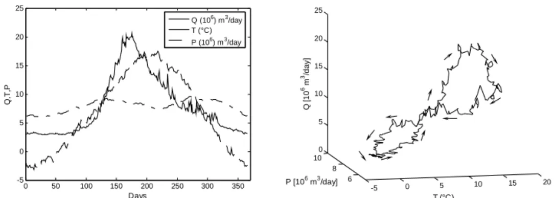
A first data analysis was made for all the variables. Data from the leap year were redistributed in order to reset all time sequences to have 365 data points. Precipitation and temperature were spatially averaged, and a time average of the year-to-year daily data was then made in order to obtain a representative set of the typical interannual basin behavior. Eventually, in order to extract the seasonal component that characterizes precipitation, a moving average with a running window equal to 91 days was applied to the data. This window has been proved to be an optimal compromise to extract the seasonal component without smoothing the series too much (Saltzman 1983). The resulting typical annual behaviour is shown in Figure 2. We call this set of data the “training set”. Notice the typical periodicity characterizing both temperature and stream-flows. The central part of the year shows an evident maximum dictated by the warmer season. In such basins, temperature drives the melting of the snow and is responsible of the earlier maximum of river runoff. Melting of ice, which represents the old water, occurs later and tends to bring the flow in phase with temperature. Also, is worth noting the behavior of the autumnal river runoff when temperatures are still above zero.
0 50 100 150 200 250 300 350 -5 0 5 10 15 20 25 Days Q, T ,P Q (106) m3/day T (°C) P (106) m3/day -5 0 5 10 15 20 6 8 10 0 5 10 15 20 25 T (°C) P [106 m3/day] Q [1 0 6 m 3/day]
Figure 2. Mean annual hydro-climatic behaviour of the Valle d’Aosta basin. (Left panel) The
training data set of precipitation (p) , temperature (T) and streamflow (Q). (Right panel) Corre-sponding trajectory in the state space of three variables p,T,Q: arrows indicate evolution.
3. Reconstructing differential equations from time series
We now build up a 2-D nonlinear differential model forced by two exogenous variables (Figure 3). The aim is to obtain for each equation a simple polyno-mial form involving the hydrological variables up to a certain algebraic degree. Both p(t) and T(t) are considered as being the independent forcing actions. We start by expressing the volume V and the runoff Q in the outlet section as,
). , ( ) , ( V T Q Q Q p V V = = (1a,b)
By differentiating the previous equations and taking advantage of the continu-ity equation for the basin we have
. dt dV V Q dt dT T Q dt dQ Q p dt dV T V ∂ ∂ + ∂ ∂ = − = (2a,b)
In Eq. 2a we deliberately neglected contributions by evaporation, evapotranspi-ration and deep infiltevapotranspi-ration. An explicit form for the second equation can be obtained by considering the data plots in the planes (Q,T) and (Q,V) and as-suming a possible dependence on the two variables V and T . Note that the two equations are coupled by a physical condition that assures the continuity of mass over the domain. While details are reported elsewhere (Perona et al., in preparation), here we show the mathematical form of the resulting differential model . 7 2 6 5 4 3 2 1V c VQ cVp c VT c p cVT c Q c dt dQ Q p dt dV + + + + + + = − = (3a,b)
This is a nonlinear model in the state variables (V, Q), parsimonious in the number of involved coefficients ci, and forced by the presence of the
exoge-nous variables p(t) and T(t). The second equation accounts for nonlinear effects in the product of the two state variables, as well as non-linearities that are
im-) , ( ) , ( V T Q Q Q p V V = = & & 0 50 100 150 200 250 300 350 400 2 4 6 8 10 12 14 16 18 20 22 Streamflow output 0 50 100 150 200 250 300 350 400 5.5 6 6.5 7 7.5 8 8.5 9 9.5 10 Precipitation input 0 50 100 150 200 250 300 350 400 -5 0 5 10 15 20 Temperature input
plicitly contained in the non-homogeneous terms. Such an equation therefore represents a precipitation-storage-runoff transformation in the form of a set of coupled nonlinear ordinary differential equations.
Model coefficients have been estimated using the “Trajectory Method” (Eisen-hammer et al. 1991), which has the peculiarity of considering at the same time the short and long-term behavior of the system trajectory in the corresponding phase space (see also, Perona et al. 2000). First of all, the phase space trajec-tory of Figure 2 has been interpreted as being periodic and a sequence of 20 years was built. This step, as well as the presence of some irregularity in the data are important for the learning procedure, and make the extracted model more robust against forcing (Perona et al. 2000). After having chosen several initial conditions xrj≡(Vj, Qj) on the phase space trajectory and fixed a trial set
of coefficients ci, the method uses Equations (3) and the values of the
exoge-nous variables (p(t), T(t)) to obtain an estimate of the successive states of the system xm(tj+∆tl)≡(V(tj+∆tl), Q(tj+∆tl)) where ∆tl =h2(l-1), with l=1,..., lmax. In
this way a quality function W can be constructed,
∑ ∑
= = ∆ + − ∆ + = max max 1 1 ) ( ) ( j j l l l j r l j m t t t t W x x , (4)where ||•|| is the euclidian norm and xm , xr are the modeled and real states. The
parameter ∆tl represents the extent to which the medium and long-term
behav-ior of the system is considered starting from jmax initial conditions. Thanks to
the already know form of the continuity equation (3a), the problem reduces here to the scalar form
. ) ( ) ( ) ( max max 1 1 2
∑ ∑
∫
= = ∆ + ⎥ ⎥ ⎦ ⎤ ⎢ ⎢ ⎣ ⎡ ∆ + − + = j j l l l j r j m t t t m d Q t Q t t Q W l j j τ τ & (5)The optimum values of the coefficients ci are obtained by minimizing the
qual-ity function (5) using the least-square method, i.e. iteratively looking for the condition in the linear space of the coefficients. The reader is referred to Perona et al. (2000) for details.
W W i c min min =
4. Results and model performances
The reconstruction technique was performed using different combinations of the method’s parameters (i.e., jmax, lmax, d), and starting with an initial
condi-tion for the reconstructed stored volume equal to 7000⋅107
m3. This volume was roughly estimated based on the current snow and ice reserves of the Valle d’Aosta region. Figure 4 shows a compilation of reconstruction sequences per-formed on the training set. The mechanism with which the model learns about the system dynamics is thus evident. In panel (a) the trial set of coefficients gives an unstable model, regardless of the initial condition from which the model starts on. After a few iterations the current set of coefficients already
al-lows for a better approximation of the phase space trajectory (panel b). Things improve with successive iterations (panel c); the procedure is then
65000 6600 6700 6800 6900 7000 7100 7200 7300 7400 7500 5 10 15 20 25 V [107 m3] Q [1 0 6 m 3/d a y ] 65000 6600 6700 6800 6900 7000 7100 7200 7300 7400 7500 5 10 15 20 25 V [107 m3] Q [1 0 6 m 3/d a y ] 65000 6600 6700 6800 6900 7000 7100 7200 7300 7400 7500 5 10 15 20 25 V [107 m3] Q [1 0 6 m 3/day ] 65000 6600 6700 6800 6900 7000 7100 7200 7300 7400 7500 5 10 15 20 25 V [107 m3] Q [ 1 0 6 m 3/day] (a) (b) (d) (c)
Figure 4. Reconstruction of model’s coefficients via successive iterations. (a) trial set of
coef-ficients at the first run, where the model’s behaviour (broad line) is evidently different from the observed one (thin line). (b) Fifth iteration, (c) tenth and (d) the fiftieth one when the proce-dure was stopped.
stopped as soon as coefficients do not appreciably change with further itera-tions (panel d).The scenario described by Figure 4 is essentially the same when the procedure parameters are changed. Only minor differences would result, for instance in the extent of the model trajectory (i.e, shorter or longer depend-ing on the parameter lmax), the number of initial conditions (i.e., decided upon
changing jmax), and the frequency with which this latter are chosen (i.e.,
pa-rameter d that fixes the distance between them). The reconstruction is likely to be successful within a specific range of such parameters (see, Perona et al. (2000) for details). From each reconstruction, seven coefficients were ob-tained; their average is shown in Table I.
The model with the coefficients of Table I reproduces the training set of data well (Figure 5a,b). While the shape of the mean annual behaviour of stream-flow is well reproduced, some of the residual oscillations that still characterize it are instead automatically smoothed. That is, the model catches the main be-haviour underlined in the data and, at the same time, seems to endure high fre-quency oscillations. Unlike some previous efforts (see, Perona et al 2000), a considerable advantage of inferring the structure of the model since the begin-ning is the intrinsic robustness that the model develops against dynamical noise. This indicates the possibility of reproducing the basin behavior not only
Table 1. Averaged numerical value of the model coefficients corresponding to the 15 best
re-construction performed with different parameters (jmax, lmax).
c1 c2 c3 c4 c5 c6 c7 1.0437⋅10-5 1.6935⋅10-4 -8.9120⋅10-5 5.9776⋅10-7 6.4442⋅10-1 3.8864⋅10-7 -1.2518⋅100 0 50 100 150 200 250 300 350 -5 0 5 10 15 20 25 Days Q, T,P Q (106) m3/day T (°C) P (106) m3/day 0 50 100 150 200 250 300 350 6600 6700 6800 6900 7000 7100 7200 7300 7400 7500 Days V V (107) m3 Reconstructed (a) (b) 18000 2000 2200 2400 2600 2800 3000 5 10 15 20 25 30 35 Days Q Original (106) m3/day Reconstructed 18000 2000 2200 2400 2600 2800 3000 5 10 15 20 25 30 35 40 45 50 Days Q Original (106) m3/day Reconstructed (c) (d)
Figure 5. Comparison between the observed data (precipitation smoothed with a 91 day
mov-ing average), and the modeled one. (a) Snapshot of the three time series of precipitaton, tem-perature and streamflow and related comparison for this latter; (b) Reconstructed volumes on the basin. Model behaviour when used to mimic daily streamflow starting from more or less filtered data of precipitation and temperature: (c) 31 days moving average and (d) original daily data.
when inputs are not periodic, but also when they contain natural oscillations as those appearing at weekly and daily time scales. This is shown in Figures 5c,d: three consecutive years of simulation and the comparison with observations are shown in panel c and d. These results come from using either smoothed (31 days m.a.) or original daily data of precipitation and temperatures as new in-puts to the model. The comparison is satisfactory, albeit some significant dif-ferences are still evident for large events. However, the purpose of such model is not to have a tool for short terms prediction, but to have a determinist tool, which is robust enough against forcing, and is thus able to infer some clues about the system behaviour at a longer term.
The model represents a dissipative nonlinear dynamical system as can be seen by rewriting the equation as a canonical non-homogeneous 2nd order ODE (Perona et al., in preparation). This system has a periodic attractor (i.e., a limit cycle of period one) when forced with the “training” data set. Viceversa, for hypothetic vanishing precipitation, the system possesses an invariably stable equilibrium point at zero. The high sensitivity of such systems versus
precipi-tation (Dingman 2002), allows for other scenarios where periodic or quasi-periodic attractors can be obtained depending on the forcing characteristics and frequency (Perona et al., in prepar.). The possibility that transition to chaos oc-curs is also being investigated, as well as the effects of trends in the inputs. Figure 6 shows, for instance, the transitory induced by a weak linear trend in the historical data (here positive for temperature and
0 1000 2000 3000 4000 5000 6000 7000 8000 5000 5500 6000 6500 7000 7500 8000 Days V 0 1000 2000 3000 4000 5000 6000 7000 8000 0 5 10 15 20 25 30 Days Q (a) (b)
Figure 6. Effects of linear trends in the inputs in the resulting volume (a) and streamflow (b)
evolution. In this case for an increase of 2 degrees over 30 years and a 20 % reduction in pre-cipitation volume, the model foresees a 15% reduction of the stored volume.
negative for precipitation) on the stored volumes and the corresponding river runoffs. Further analyses are being explored (Perona et al., in preparation).
5. Conclusions
The possibility of reconstructing a meaningful mechanistic model to reproduce the complex dynamics of alpine basins has been described in this work. Recon-structing the lumped input-outputs dynamics by exploring the trajectories of the system in the phase space allows the differential model to experience the effects induced by noise in the inputs directly. This makes it robust and attrac-tive with regard to future speculaattrac-tive and applied works. Speculaattrac-tive will aim at characterizing the system under a more dynamical viewpoint; applied works will look at the possibility of assessing the future system behaviour, as well as transferring the present approach to other alpine basins.
References
Corripio, J. G., and R.S. Purves, 2005: Surface energy balance of high altitude gla-ciers in the Central Andes: the effect of snow penitents, in Climate and Hydrology
in Mountain Areas, Edited by de Jong, C., Collins, D, Ranzi, R., John Wiley &
Sons, 15-27.
Dingman, S. L. Physical hydrology, Second Edition, Prentice Hall, New Jersey, 2002; Eisenhammer, T., A. Hübler, N. Packard, and J.A.S. Kelso, 1991: Modeling
experi-mental time series with ordinary differential equations, Biological cybernetics, 65, 107-112.
Ohmura, A., 2001: Physical basis for the temperature-based melt-index method,
Jour-nal of Applied Meteorology, 40, 753-761.
Perona, P., A. Porporato, and L. Ridolfi, 2000: On the Trajectory Method for the re-construction of differential equations from time series. Nonlinear Dynamics, 23, 13-33.