Multi-site CO₂ sequestration optimization using a dynamic programming approach

(1)

Multi-site CO

2

Sequestration Optimization using a Dynamic

Program-ming Approach

Brent Cody1, Ana González-Nicolás2, and Domenico Baù3

Civil and Environmental Engineering Department, Colorado State University

Abstract. Increased greenhouse gas emissions, resulting from our heavy dependence upon fossil fuels, have been found to be directly related to global warming. Global warming may lead to adverse conditions, such as the melting of polar ice caps, raised ocean levels, as well as altered weather patterns producing higher intensity hurricanes and storms. While technological advances, public education, and enacting policy changes are excellent long-term solutions to this problem, carbon sequestration (CS) in addition to other short term solutions may provide a bridge to a sus-tainable future. Unfortunately, leakage of sequestrated CO2 may contaminate air and water

re-sources as well as adversely affect plant and animal life. These risks must be fully understood and minimized before implementation.

A preliminary decision support system (DSS) has been constructed to optimize CS at a given number of potential injection sites, with the goal of minimizing the total cost of CO2 leakage while

meeting a specified sequestered mass target. This DSS uses a graphic user interface (GUI) and employs CSUDP, a generalized dynamic programming software, as an optimization driver. A semi-analytical leakage model was integrated into CSUDP’s objective function to estimate leakage costs. Based upon work by Nordbotten et al. (2009), this model quantifies the mass of CO2 leakage

through weak areas, such as abandoned oil wells, of the caprock overlying the injected aquifer. The resulting DSS uses a wide range of geological, economical, and infrastructural parameters to output optimal CO2 injection rates and injection durations for each site.

1. Introduction

The average CO2 concentration in the atmosphere has increased from approximately 280 to 385 ppm over the last 250 years. Approximately two thirds of this increase has oc-curred in past 60 years (Keeling and Whorf, 2000). These increased greenhouse gas emis-sions have been found to be related to global warming (Ledley et al., 1999). CS may help to provide a short term solution of reducing greenhouse gas emissions.

CS prevents CO2 from entering the atmosphere by capturing it at emission sites (coal power plants, manufacturing sites, etc.), compressing it into a supercritical phase, and in-jecting it into deep, unusable aquifers where, ideally, it will remain for an indefinitely long time period. Unfortunately, this technology is relatively new and its long and short term risks must be minimized. It is possible for sequestrated CO2 to migrate through the subsur-face and eventually reach usable ground water resources or even the ground sursubsur-face. Leakage of sequestrated CO2 may contaminate air and water resources, as well as adverse-ly affect plant and animal life (Bachu, 2003). Before implementation of CS technologies, these risks must be fully understood and minimized.

1_e-mail:_{codybm@engr.colostate.edu} 2_e-mail:_{anagna@hotmail.com} 3 _e-mail:_{domenico.bau@colostate.edu}

(2)

Cody, Gonzalez-Nicolas and Baú

Several past studies have applied optimization methods to CS. The most common form of optimization studies in this field have focused upon using CO2 injection for en-hanced oil recovery. For example, Babadagli (2006) used numerical models to compare multiple injection/recovery strategies. Others focused on optimizing CO2 sequestration in-to depleted oil reserves. Han (2009) used numerical models in-to test the feasibility of se-questering CO2 below depleted oil reservoirs and compare competing properties and pro-cesses. There are also several studies (Akimoto et al. 2004; Keller 2008) attempting to timize the large scale economics of CS. Middleton (2009) attempted to economically op-timize CO2 source outputs with prospective CS sink capacities as well as transport pipeline sizing and location. To the best of the authors’ knowledge there are no studies to date which consider the risk of CO2 leakage resulting from CS as a one of the management tar-gets.

The present work attempts to address risk of CO2 leakage by minimizing a penalty, re-ferred to as the leakage cost. The leakage cost is calculated as a function of the total mass of CO2 leakage resulting from sequestering a specified mass of CO2 into multiple potential injection sites. Governmental agencies wishing to employ CS technologies may have sev-eral injection sites available and, although sevsev-eral of the parameters affecting the cost of carbon dioxide leakage are non-variable, the rate and duration of injection may be con-trolled by project planners. A DSS may thus be beneficial in choosing injection rates and injection durations for each site which i) minimizes the total cost of carbon dioxide leakage and ii) meets the total targeted storage of carbon dioxide.

In this work, a user-friendly DSS has been constructed which is able to optimize injec-tion rates and durainjec-tions at each locainjec-tion in a series of potential injecinjec-tion sites. This DSS stems from the combination of CSUDP with a semi-analytical leakage model that esti-mates leakage costs.

This article is organized as follows. Section 2 provides details of the simulation-optimization framework for the DSS. Sections 3 and 4 give a detailed description and dis-cussion of the results obtained from three hypothetical simulation-optimization tests. The extent and origin of site characteristics and parameters are explained. Also, an analysis of the effects of several parameters upon the injection strategy is presented. Section 5 summa-rizes the work to date and suggests possible future improvements. Details concerning use of the DSS may be found in Appendix A.

2. Simulation-Optimization Framework

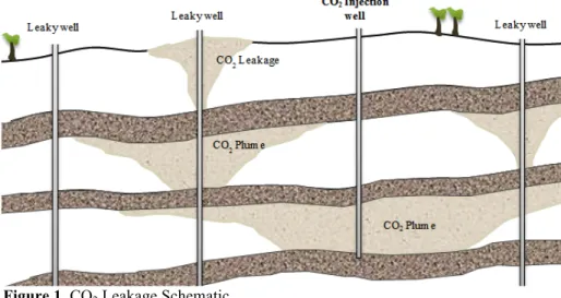
Consider that a hypothetical governmental agency wishing to employ CS has several suitable injection sites. The subsurface geology of these injection sites consist of multiply horizontal aquifer-aquitard layers (see Figure 1 below). The goal is to find an optimal in-jection strategy in these candidate sites which:

1) Minimizes the total cost of CO2 leakage using rate of injection and injection dura-tion as decision variables;

2) Sequesters the total targeted mass of CO2.

The solution to this problem may be addressed by embedding a simulation model into an optimization algorithm. These two tools are presented in the following.

(3)

2.1. Semi-Analytical Leakage Model

As seen in Figure 1, CO2 sequestered into deep aquifers can migrate to the surface through abandoned oil wells or weak areas in aquitards separating aquifer layers. A relia-ble, yet efficient, method of quantifying the mass of CO2 leakage for a given injection rate and injection duration must be determined before optimizing a multi-site injection strategy.

Figure 1. CO2 Leakage Schematic

A semi-analytical leakage model using a wide range of geological and infrastructural parameters (Table 1) was employed to accomplish this task. Based upon works by Nord-botten and Celia (2006, 2009), this model quantifies the mass of CO2 leakage through weak areas in the system’s aquitards, referred to herein as ‘leaky wells’, for subsurface sys-tems containing multiple aquifer-aquitard layers and multiple leaky wells.

This algorithm stems from several simplifying assumptions. Some of the most im-portant of these assumptions are:

• All aquifers are initially saturated with water;

• All aquifers are horizontally level, homogenous, and isotropic; • All aquitards are impermeable, except where there is a leaky well; • Injection and leakage rates for each time step are constant;

• System matrix and fluids are slightly compressible; • Capillary forces are ignored.

(4)

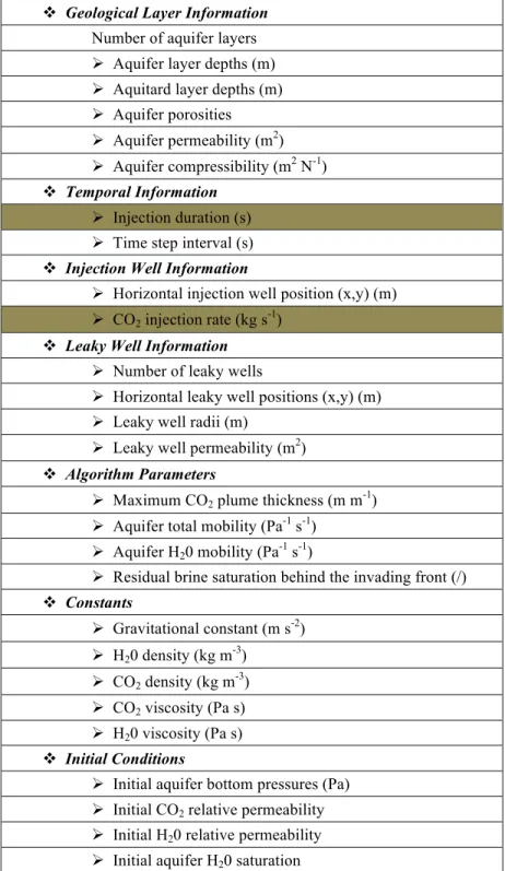
Table 1. Model Input Parameters with Decision Variables Highlighted Brown

v Geological Layer Information Number of aquifer layers Ø Aquifer layer depths (m) Ø Aquitard layer depths (m) Ø Aquifer porosities Ø Aquifer permeability (m2₎

Ø Aquifer compressibility (m2_N-1₎

v Temporal Information Ø Injection duration (s) Ø Time step interval (s) v Injection Well Information

Ø Horizontal injection well position (x,y) (m) Ø CO2 injection rate (kg s-1)

v Leaky Well Information Ø Number of leaky wells

Ø Horizontal leaky well positions (x,y) (m) Ø Leaky well radii (m)

Ø Leaky well permeability (m2₎

v Algorithm Parameters

Ø Maximum CO2 plume thickness (m m-1)

Ø Aquifer total mobility (Pa-1_s-1₎

Ø Aquifer H20 mobility (Pa-1 s-1)

Ø Residual brine saturation behind the invading front (/) v Constants Ø Gravitational constant (m s-2) Ø H20 density (kg m-3) Ø CO2 density (kg m-3) Ø CO2 viscosity (Pa s) Ø H20 viscosity (Pa s) v Initial Conditions

Ø Initial aquifer bottom pressures (Pa) Ø Initial CO2 relative permeability

Ø Initial H20 relative permeability

(5)

According to Nordbotten and Celia (2006), the pressure distribution of two-phase flow in the injected formations relies upon the following differential equation, derived from principles of mass conservation, energy minimization and Darcy flow:

⎥ ⎦ ⎤ ⎢ ⎣ ⎡ Γ + + − = − χ χ λ λ χ 2 1 ' ' 1 ) 1 ( ' 1 ' d dh h h d dp (1) where, ⎪ ⎪ ⎩ ⎪ ⎪ ⎨ ⎧ ≥ < < ⎟⎟⎠ ⎞ ⎜⎜⎝ ⎛ − − ≤ = − ≡ ≡ Δ ≡ Γ ≡ − ≡ . 2 for 0 2 2/ for 1 2 1 1 2/ for 1 ' ) 1 ( 2 , 2 ' , ) ( ' 2 2 λ χ λ χ λ χ λ λ λ χ πφ χ λ λ λ λ ρ π ρ ρ α α h t Q r S H Q H gk H h h gH p p i res w c w c w

In these equations, the subscript α denotes fluid type (w = water and c = CO2), λ is the fluid mobility (λα = kr,α/µα), krα is the relative permeability, µα is the dynamic viscosity, φ

is the aquifer porosity, H is the aquifer depth, Sres is the residual water saturation behind

the invading CO2 front, ri is the radius of well i, Q is the mass flow rate into the aquifer, ρ

is the fluid density, g is the gravitational constant, and k is the aquifer permeability. The pressure solution throughout the domain is found by integrating Equation (1):

(

)

[

]

(

)

(

)

[

]

(

)

[

]

⎪ ⎪ ⎪ ⎪ ⎪ ⎪ ⎪ ⎪ ⎩ ⎪⎪ ⎪ ⎪ ⎪ ⎪ ⎪ ⎪ ⎨ ⎧ ≥ < ≤ − ⎟⎟⎠ ⎞ ⎜⎜⎝ ⎛ Γ − < < − ⎪⎭ ⎪ ⎬ ⎫ ⎪⎩ ⎪ ⎨ ⎧ ⎥ ⎥ ⎦ ⎤ ⎢ ⎢ ⎣ ⎡ − ⎟ ⎠ ⎞ ⎜ ⎝ ⎛ Γ − ⎪⎭ ⎪ ⎬ ⎫ ⎪⎩ ⎪ ⎨ ⎧ − ⎟⎟⎠ ⎞ ⎜⎜⎝ ⎛ + ⎥ ⎥ ⎦ ⎤ ⎢ ⎢ ⎣ ⎡ ⎟ ⎠ ⎞ ⎜ ⎝ ⎛ − − + ≤ − ⎟⎟ ⎟ ⎟ ⎠ ⎞ ⎜⎜ ⎜ ⎜ ⎝ ⎛ Γ − = ψ χ ψ χ λ ρ ρ ψ χ λ χ λ ρ ρ λ χ χ λ λ χ λ λ λ χ ρ ρ λ χ λ for 2 for ln 2 1 2 2/ for * 1 2 1 1 2 2 ln 1 2/ for 2 ln 2 1 ) ; , ( 0 0 5 . 0 5 . 0 5 . 0 2 1 2 p gH p gH p gH p t z r p c w c w c w (2) where,

(6)

(

)

[

]

(

)

[

(

)

]

. ~ ~(1 ) 4.5 1 2 2 1 1 2 2 2 2 ln 1 2 ln 2 1 ) 0 ; , ( 5 . 0 5 . 0 5 . 0 2 1 2 0 1 0 w w c c eff res w c w c w Q Q Q Q c S K H gH p p gH p p t z r p p ρ ρ φλ π ρ ρ λ λ λ λ λ λ λ λ ρ ρ ψ λ + ≡ − ≡ Ψ − ⎪ ⎪ ⎭ ⎪ ⎪ ⎬ ⎫ ⎪ ⎪ ⎩ ⎪ ⎪ ⎨ ⎧ ⎥ ⎥ ⎥ ⎥ ⎦ ⎤ ⎢ ⎢ ⎢ ⎢ ⎣ ⎡ − ⎟⎟ ⎟ ⎟ ⎠ ⎞ ⎜⎜ ⎜ ⎜ ⎝ ⎛ Γ − ⎪ ⎪ ⎭ ⎪⎪ ⎬ ⎫ ⎪ ⎪ ⎩ ⎪⎪ ⎨ ⎧ − ⎟⎟ ⎟ ⎟ ⎠ ⎞ ⎜⎜ ⎜ ⎜ ⎝ ⎛ + ⎥ ⎥ ⎥ ⎥ ⎦ ⎤ ⎢ ⎢ ⎢ ⎢ ⎣ ⎡ ⎟⎟ ⎟ ⎟ ⎠ ⎞ ⎜⎜ ⎜ ⎜ ⎝ ⎛ − − + = − ⎟⎟⎠ ⎞ ⎜⎜⎝ ⎛ Γ − = = =

In the above equations ceff is the effective compressibility of the system. According to

Nordbotten and Celia (2009), leaky well flow rates across each aquitard can be determined as: ⎟⎟⎠ ⎞ ⎜⎜⎝ ⎛ − ₊ − = + − g B p p k k r Q _l l T l B r l w w α α α α α π 2 _µ ρ ρ (3)

where pBl+ and pTl- denote the fluid pressures directly above and below the aquitard,

re-spectively, kwl is the leaky well’s water saturated permeability at aquitard layer l, and B is

the aquitard thickness. Equation (3) assumes that CO2 flow at each well begins upon plume arrival. After subdividing the injection time horizon into a finite number, nts, of time steps,Δ , the mass of CO2 leakage, Mleak, into a prescribed aquifer, L, overlying the t

injected formation may be calculated as:

∑∑

= = _Δ = nts ts nw i L l i ts c t Q Mleak 1 , , ₍₄₎

where w is the leaky well index, and nw is the number of leaky wells.

The semi-analytical model estimates CO2 mass leakage using the following steps: 1. The pressure distribution is found throughout the domain at the end of the current

time step using Equation (2).

2. Leaky well flow rates are found for the next time step using Equation (3).

3. The total CO2 leakage mass is obtained as the sum of each time step’s CO2 leakage mass into the top geological layer using Equation (4).

This semi-analytical model needs to be calibrated with site data before being used for real-world decision-making purposes. Additionally, the solution is not accurate if its un-derlying assumptions are grossly violated. In this case, a more accurate, yet computation-ally costly, numerical model must be applied.

(7)

2.2 Dynamic Programming and CSUDP

The semi-analytical model described above returns the mass of CO2 leakage for a spec-ified injection time and duration (Equation (4)), however, this model turns out to be highly non-linear and mildly computationally intensive. A dynamic programming (DP) approach is used as a method of finding a global injection scheme that minimizes the total cost of leakage over a number of potential injection sites.

DP is used to separate a large problem into several smaller problems. Unlike several optimization methods, it uses discrete rather than continuous variable ranges. In our prob-lem, the mass of CO2 that each site is able to sequester ranges between 0 and a specified upper bound. This range is then discretized using a specified interval. For example, sup-pose an injection site is able to hold 40 million kg of CO2 and the discretization interval is set at 20 million kg. This would result in three injection options for this site; 0 kg, 20 mil-lion kg, or 40 milmil-lion kg. As expected, the computational cost and accuracy of the DP method are directly related to the size of the discretization interval of the considered deci-sion variable.

Site locations, as opposed to DP’s more typical method of using time steps, are defined as stages. That is, in a forward-looking DP method, leakage costs for all feasible injection quantities are calculated for each injection site starting at the initial site and continuing to the final site. The remaining mass of CO2 to be sequestered (kg) after injection into pre-ceding sites is defined as the state variable. The state variable is initially set at the speci-fied sequestered mass target and must be reduced to zero after the final stage. This simply means that the entire specified sequestered mass target must be distributed and sequestered into the injection sites.

The objective function represents CO2 leakage cost ($), as is specified below, as a non-linear function of the mass CO2 leakage found using Equation (4). DP optimization finds a minimal objective function value while reducing the state variable to zero after looking at all possible injection sites (stages):

⎭ ⎬ ⎫ ⎩ ⎨ ⎧ ₌

_∑

= n i p i iMleak i c t LeakageCos Objective 1 min : (5a) max 0 : 1 Q Q Constraint ≤ _inj≤ (5b) max 0 : 2 T T Constraint ≤ ≤ (5c) max 0 : 3 t t Constraint ≤ _start ≤ (5d) . 0 : 4 t t_max

Constraint ≤ _end ≤ (5e)

end start t

t

Constraint5: ≤ (5f)

In Equation (5), LeakageCost is the total cost ($) incurred from CO2 leakage, n is the number of injection sites (or stages), i is the site (or stage) index, ci is the cost per unit

mass ($ kg-pi_{) for well i, Mleak}_i_{is the mass (kg) of CO}_{2 leakage for well i, p}_i_{is a nonlinear} leakage cost coefficient for well i, Qinj is the rate (kg s-1) of CO2 injection, Qmax is the

max-imum rate of CO2 injection, T is the targeted mass (kg) of CO2 to be sequestered, Tmax is

the maximum CO2 mass target, and tmax is the maximum time of simulation. Injection

(8)

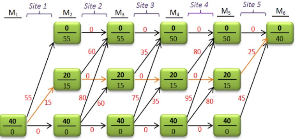
A simple example (see Figure 2) may provide clarification of the DP approach. In Figure 2, the bold black font numbers represent the state variable, or the mass of CO2 yet to be injected (i.e. 0, 20 million, or 40 million kg). The costs of reducing the state variable by injecting CO2 into each site are represented in red font, and the current objective value (or cost incurred after sequestering into previous sites) may be found below the line in each box in standard black font. For a minimization project, if multiple arrows (choices) inter-sect the left side of a box (state), DP uses the choice resulting in the lowest incurred cost for the current stage and state.

Figure 2. Dynamic Programming Schematic. CO2 masses (in bold black

font) are in millions of kg and costs (in red and standard black font) are in thousands of $

In the example shown in Figure 2, there are initially 40 million kg of CO2 to sequester. Site 1 is first location to be analyzed. The options are to inject 0, 20 million, or 40 million kg, with hypothetical leakage costs of $0, $15,000, or $55,000, respectively. Next, for Site 2, the options are to inject 0, 20 million, or 40 million kg, with leakage costs of $0,

$60,000, or $80,000, respectively. The objective values for each state cannot be improved by sequestering CO2 into Site 2. For Site 3, an injection of 0, 20 million, or 40 million kg produces leakage costs of $0, $35,000, or $70,000, respectively. The DP approach is thus able to reduce the objective function at “state 0” from $55,000 to $50,000 by injecting 20 million kg into Site 1 and 20 million kg into Site 3. The method continues analyzing the remaining sites looking for an injection strategy that results in the minimum possible leak-age cost. In this example, the optimum injection strategy, represented by orange arrows in Figure 2, is to inject 20 million kg into Site 1 and 20 million kg into Site 5, resulting in a total leakage cost of $40,000.

The actual DP routine looks at a much larger range of the state variable (0 to 1.58 x 1011 kg) with a more representative discretization interval. CSUDP is a dynamic pro-gramming software developed by Labadie (1999). Because CSUDP is quite general, sev-eral user options must be specified. Ranges and discretization intervals must be set for both decision and state variables. Also, three user function files must be produced; the state function, objective function, and read-in function. The state and objective function files govern how costs are calculated while the read-in function assigns data from input files to variables.

Figure 2. Dynamic Programming Schematic. CO2 masses (in bold black

font) are in millions of kg and costs (in red and standard black font) are in thousands of $

In the example shown in Figure 2, there are initially 40 million kg of CO2 to sequester. Site 1 is first location to be analyzed. The options are to inject 0, 20 million, or 40 million kg, with hypothetical leakage costs of $0, $15,000, or $55,000, respectively. Next, for Site 2, the options are to inject 0, 20 million, or 40 million kg, with leakage costs of $0,

$60,000, or $80,000, respectively. The objective values for each state cannot be improved by sequestering CO2 into Site 2. For Site 3, an injection of 0, 20 million, or 40 million kg produces leakage costs of $0, $35,000, or $70,000, respectively. The DP approach is thus able to reduce the objective function at “state 0” from $55,000 to $50,000 by injecting 20 million kg into Site 1 and 20 million kg into Site 3. The method continues analyzing the remaining sites looking for an injection strategy that results in the minimum possible leak-age cost. In this example, the optimum injection strategy, represented by orange arrows in Figure 2, is to inject 20 million kg into Site 1 and 20 million kg into Site 5, resulting in a total leakage cost of $40,000.

The actual DP routine looks at a much larger range of the state variable (0 to 1.58 x 1011 kg) with a more representative discretization interval. CSUDP is a dynamic pro-gramming software developed by Labadie (1999). Because CSUDP is quite general, sev-eral user options must be specified. Ranges and discretization intervals must be set for both decision and state variables. Also, three user function files must be produced; the state function, objective function, and read-in function. The state and objective function files govern how costs are calculated while the read-in function assigns data from input files to variables.

(9)

In the considered optimization problem (Equation (5a-e)) there are infinitely many pos-sible combinations of CO2 mass injection rates and injection durations for each site. For example, an injection of 20 million kg of CO2 into Site 1 would take 10 years at 2 million kg yr-1_{, 4 years at 5 million kg yr}-1_{, or 1 year at 20 million kg yr}-1_{. All possible rate and} time combinations (using a 1 year temporal discretization between the user specified injec-tion time range) are tested for each possible CO2 injecinjec-tion mass.

In order to determine leakage costs (Equation (5a)), the semi-analytical model (Equa-tion (4)) is integrated into CSUDP. CSUDP is able to determine site specific mass leakage by reading each scenario’s input parameters. The parameters for Equation (5) are read from an input database, enabling the estimation of leakage costs from the leakage mass quantities calculated using the semi-analytical model (Equation (4)). Within the CSUDP framework, all discrete rate-duration combinations for each possible mass injection deci-sion are tested. The rate-duration combination giving the minimum cost of leakage for the site and injection quantity being analyzed is finally selected to provide the cost of leakage, i.e. the red numbers in Figure 2’s example. Once all costs are calculated, CSUDP can identify the optimal injection strategy, represented with orange arrows in Figure 2’s exam-ple.

3. DSS Procedure

Three hypothetical simulations were carried out to analyze the performance of the de-veloped DSS. Each simulation determined an optimal injection strategy for five hypothet-ical sites. Site 1 was considered as the “reference” site for each simulation. Sites 2 - 5 were “variations” of Site 1. Reference site input parameters are listed in Table 2. The co-ordinates of leaky well locations are provided in Table 3. The injection well is positioned at the origin of the reference system.

The first DSS simulation altered specific geological parameters in an attempt to deter-mine how varying aquifer and aquitard thickness would affect CO2 leakage quantities. In the second DSS simulation, the number, radii, and permeabilities of leaky wells were al-tered. For the third DSS simulation, economic parameters were varied to determine how a change in the leakage cost per unit and the leakage coefficient would affect the injection site ranking. Table 4 shows site specific parameter changes in accordance with each simu-lation.

4. Results and Discussion

4.1 Geological Parameter Testing

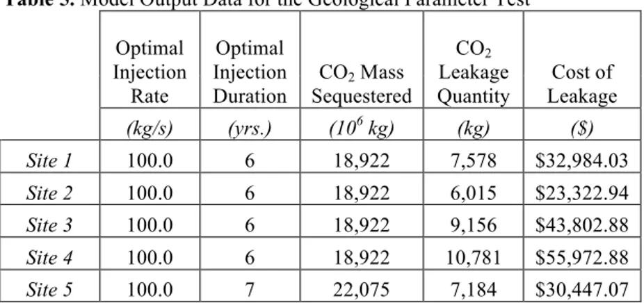
Aquifer and aquitard thickness were altered against the reference site (Site 1) with the intent of determining the effect upon CO2 leakage quantities. As shown in Table 4, the aq-uifer thickness was decreased and increased by 20% in Sites 2 and 3, respectively, whereas an aquitard thickness decrease and increase of 20% was simulated in Sites 4 and 5, respec-tively. Table 5 shows the DSS output information for this geological parameter test.

As expected aquitard thickness seems to be inversely correlated with leakage quantity and thus cost. Additionally, CO2 leakage seems to be very sensitive to aquitard thickness. Site 4 had the lowest aquitard thickness (4 m) and, although each site had an equal quantity

(10)

of mass sequestered, was estimated to leak approximately 42% more CO2 mass than the reference site.

Table 2. Model Input Parameters for the Reference Site

Sequestration Target (kg) 9.78E+10

Injection time range (yr) 6-10

Leakage Cost per Unit ($ kg-p₎ _0.05

Leakage Cost Coefficient 1.5

Number of aquifer layers 4

Aquifer layer thicknesses (m) 100

Aquitard layer thicknesses (m) 5

Aquifer porosities 0.15

Aquifer permeabilities (m2) 1.00E-11 Aquifer compressibilities (m2 N-1) 1.00E-12 Injection duration (s) Decision Variable

Time step interval (s) 3153600

Horizontal injection well position (x,y) (m) (0,0) CO2 injection rate (kg s-1) Decision Variable

Number of leaky wells 8

Horizontal leaky well positions (x,y) (m) Random Generation

Leaky well radii (m) 0.2

Leaky well permeabilities (m2₎ _1.00E-16

Maximum CO2 plume thickness (m m-1) 0.5

Aquifer total mobilities (Pa-1_s-1₎ ₁₅

Aquifer H20 mobilities (Pa-1 s-1) 20

Residual brine saturation behind the invading front (/) 0.08 Gravitational constant (m s-2) 9.81

H20 density (kg m-3) 1000

CO2 density (kg m-3) 600

CO2 viscosity (Pa s) 0.00005

H20 viscosity (Pa s) 0.0005

Initial aquifer bottom pressures (Pa) Hydrostatic with a bottom da-tum of 3000 m below surface Initial CO2 relative permeability 0.0001

Initial H20 relative permeability 1

Initial water saturation 1

Maximum CO2 injection rate (kg s-1) 100

Maximum sequestration target (kg) 1.58E+11

(11)

Table 3. Leaky Well Coordinates Well ID X (m) Y (m) 1 -9337 3663 2 3019 3898 3 -508 663 4 -651 2713 5 7145 -7270 6 -7552 7807 7 -9642 2607 8 -9516 8324 9 -9812 -8491 10 -5452 5381

Table 4. Simulation Site Parameters

Factor Tested Site 1 Site 2 Site 3 Site 4 Site 5 Geological Parameters Reference Case 20% thinner aquifers 20% thicker aquifers 20% thinner aquitards 20% thicker aquitards Leaky Well Parameters Reference Case 2 less leaky wells 2 more leaky wells 20% greater leaky well radii 20% greater leaky well conductivity Economical Parameters Reference Case 2× Leakage Cost per Unit 10× Leakage Cost per Unit 5% greater leakage co-efficient 20% greater leakage co-efficient

Table 5. Model Output Data for the Geological Parameter Test

Optimal Injection Rate Optimal Injection Duration CO2 Mass Sequestered CO2 Leakage Quantity Cost of Leakage (kg/s) (yrs.) (106_kg) _(kg) _($) Site 1 100.0 6 18,922 7,578 $32,984.03 Site 2 100.0 6 18,922 6,015 $23,322.94 Site 3 100.0 6 18,922 9,156 $43,802.88 Site 4 100.0 6 18,922 10,781 $55,972.88 Site 5 100.0 7 22,075 7,184 $30,447.07

Interestingly, aquifer thickness was found to be directly correlated with CO2 leakage quantity. Site 3 had a 20% greater aquifer thickness and leaked 21% more CO2 per mass sequestered than the reference site.

(12)

4.2 Leaky Well Parameter Testing

For the second simulation the number, radii, and permeabilities of leaky wells were al-tered against the reference site (Site 1) with the intent of determining the effect upon CO2 leakage quantities. In Sites 2 and 3 the number of leaky wells was decreased and increased by 2, respectively, while an increase of 20% in the radii of leaky wells and the well perme-abilities were simulated in Sites 4 and 5, respectively. Table 6 shows the DSS output in-formation for the leaky well parameter test.

Table 6. Model Output Data for the Leaky Well Parameter Test

Optimal Injection Rate Optimal Injection Duration CO2 Mass Sequestered CO2 Leakage Quantity Cost of Leakage (kg/s) (yrs.) (106_kg) _(kg) _($) Site 1 100.0 6 18,922 7,578 $32,984.03 Site 2 100.0 7 22,075 7,194 $30,505.70 Site 3 100.0 6 18,922 9,467 $46,059.20 Site 4 100.0 6 18,922 13,169 $75,557.30 Site 5 100.0 6 18,922 10,112 $50,843.05

The number of leaky wells was found to be directly correlated with CO2 leakage quan-tity. The two additional leaky wells in Site 3 caused a 10% increase in CO2 leakage of per mass sequestered than the reference site. The two less leaky wells in Site 2 caused a 7.5% decrease in CO2 leakage per mass sequestered than the reference site.

As expected, both leaky well radius and conductivity were found to be directly corre-lated with leakage quantity. Increasing the leaky well radii seems to have the greatest ef-fect with Site 4’s 20% increase causing a 30% increase in CO2 leakage per mass seques-tered than the reference site. A 13% increase in CO2 leakage per mass sequesseques-tered was found by increasing the leaky well permeabilities by 20% in Site 5.

4.3 Economical Parameter Testing

The final test varied economical parameters. Sites 2 and 3 had leakage cost per unit that was 2 and 10 times greater, respectively, than the reference site. The leakage coeffi-cient was increased by 5% and 20% in Sites 4 and 5, respectively. The results for the eco-nomical parameter test may be seen below in Table 7.

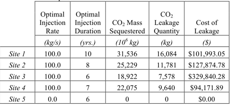
Table 7. Model Output Data for the Economical Parameter Test

Optimal Injection Rate Optimal Injection Duration CO2 Mass Sequestered CO2 Leakage Quantity Cost of Leakage (kg/s) (yrs.) (106_kg) _(kg) _($) Site 1 100.0 10 31,536 16,084 $101,993.05 Site 2 100.0 8 25,229 11,781 $127,874.78 Site 3 100.0 6 18,922 7,578 $329,840.28 Site 4 100.0 7 22,075 9,640 $94,171.89 Site 5 0.0 6 0 0 $0.00

(13)

As seen from Table 7, the leakage coefficient has the greatest affect upon the leakage cost. An increase of 20% resulted in the DSS choosing not to inject any CO2 into Site 5. In fact, an increase of only 5% resulted in a 33% reduction of mass sequestered in Site 4 from the reference site. Not surprisingly, increasing the leakage cost per unit directly in-creased the leakage cost.

5. Conclusions

A DSS has been developed and implemented to optimize CS over a number possible injection sites. CSUDP, a generalized dynamic programming tool, was used as a method of finding a global injection scheme which minimized the total cost of leakage over all possible injection sites. CSUDP called upon a semi-analytical model based upon work by Nordbotten and Celia (2009) to return the mass of CO2 leakage for a specified injection time and duration.

Three hypothetical sets of injection sites were simulated to analyze the performance of this DSS. Each test focused on a different group of parameters. The first simulation per-turbed specific geological parameters to see how varying aquifer and aquitard thickness would affect CO2 leakage quantities. The number, radii, and permeabilities of leaky wells were altered in the second simulation. The third simulation changed economic parameters in an attempt to determine how varying the leakage cost per unit and the leakage coeffi-cient would affect injection site ranking.

The results of these simulations showed relationships between the altered parameters and the mass or cost of CO2 leakage. It was found that an increase in aquifer thickness, number of leaky wells, radii of leaky wells, conductivity of leaky wells, cost per unit leak-age, or leakage coefficient caused an increase in the cost of CO2 leakage making the site less suitable to CS. An increase in aquitard thickness resulted in a decrease in the cost of CO2 leakage making the site more suitable to CS.

This prototype DSS provides a template for a general CO2 injection plan optimizer. The analytical leakage model must be first calibrated and validated against actual leakage data before applying this DSS to real-world situations.

With additional effort, the presented concept may become a valuable tool for decision makers faced with the task of sequestration site selection and identification of optimal in-jection well locations. This may possibly be achieved by coupling the dynamic program-ming optimizer with evolutionary algorithms, although the computational cost is bound to significantly increase. The application of stochastic dynamic programming may also be useful as several variables such as leaky well permeabilities and aquifer porosities may be known with uncertainty.

Acknowledgements. This research was supported by the U.S. Department of

Energy-NETL Office (Grant DE-FE0001830). The authors wish to extend their continued appre-ciation.

References

Akimoto, K. et al. (2003). “Evaluation of carbon dioxide sequestration in Japan with a mathematical model” Energy, 29, 1537-1549.

Bachu, S. (2003). “Screening and ranking of sedimentary basins for sequestration of CO2 in geological media

(14)

Babadagli, T. (2006). “Optimization of CO2 injection for sequestration / enhanced oil recovery and current

status in Canada” Advances in the Geological Storage of Carbon Dioxide, 261-270.

Celia, M.A. and Nordbotten, J.M. (2009) “Practical modeling approaches for geological storage of carbon dioxide” Ground Water, 47(5), 627-638.

Han, W.S. and McPherson, B.J. (2009) “Optimizing geological CO2 sequestration by injection in deep saline

formations below oil reservoirs” Energy Conservation and Management, 50, 2570-2582.

Keeling C. D. and T. P. Whorf (2000). “Atmospheric CO2 Records from Sites in the SIO Air Sampling

Net-work,” in Carbon Dioxide Information Analysis Center, Trends: A Compendium of Data on Global Change, Oak Ridge, TN: Ridge National Laboratory.

Keller, K., McInerney, D., and Bradford, D.F. (2008) “Carbon dioxide sequestration: how much and when?” Climate Change, 88, 267-291.

Labadie, J. (1999) “Generalized dynamic programming package: CSUDP” Documentation and user manual, Department of Civil Engineering, Colorado State Univ., Ft. Collins, CO.

Ledley, T. S., Sundquist, E. T., Schwartz, S. E., Hall, D. K., Fellows, J. D., and Killeen, T. L. (1999). Cli-mate change and greenhouse gases. EOS, Trans. AGU, 80(39), 453-458.

Middleton, R.S., and Bielicki, J.M. (2009) “A comprehensive carbon capture and storage infrastructure mod-el” Energy Procedia, 1, 1611-1616.

Nordbotten, J.M., Celia, M.A., and Bachu, S. (2004) “Analytical solutions for leakage rates through aban-doned wells” Water Resources Research, 40, W04204.

Nordbotten, J.M. and Celia, M.A. (2006) “Similarity solutions for fluid injecttion in confined aquifers” J. Fluid Mech., 561, 307-327.

Nordbotten, J.M. and Celia, M.A. (2009) “Model for CO2 leakage including multiple geological layers and

(15)

Fig. 1. Dynamic Programming Schematic

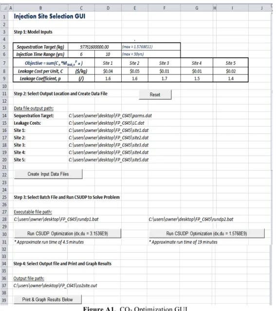
Figure A1. CO2 Optimization GUI

Appendix A

The DSS consists of a Microsoft Excel file having 6 worksheets. Worksheets 2-6 are the database for this DSS and contain the semi-analytical model’s site specific geological, infrastructure, and algorithm parameters previously listed in Section 2.1. The first work-sheet contains a GUI. As seen in Figure 3, the GUI is divided into four steps: 1) Enter model input values, 2) Generate input data files, 3) Run CSUDP, and 4) Output results.

Figures A1-A4 provide an illustration of how the GUI is operated. The user must first specify the targeted mass of CO2 for sequestration, a range of time in which to accomplish this, and the ten cost function parameters. After entering the model inputs, a button is pushed for each step with the selection of the level of accuracy in Step 3 being the only remaining user decision. Figure A2 shows the user creating all required input files by pushing the ‘Create Input Data Files’ button.

(16)

Figure A3. Run CSUDP Figure A2. Generate Input Files

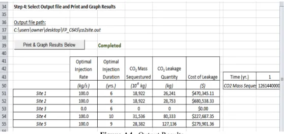
The executable CSUDP file can be seen running in Figure A3. In this step the user has the option of a 3.1536 x 109 kg or 1.5768 x 109 kg discretization interval. The finer dis-cretization interval gives more accurate results but requires more time (~20 minutes as op-posed to 5 minutes on a standard laptop). Finally, the user is able to output the results in tabular form (Figure A4) and in plot form (Figures A5-A12). The Reset button should be used to reset all “Completed” notifications and outputted values and plots before running the next simulation.

(17)

Figure A4. Output Results

Figure A5. Sequestered Mass vs. Time

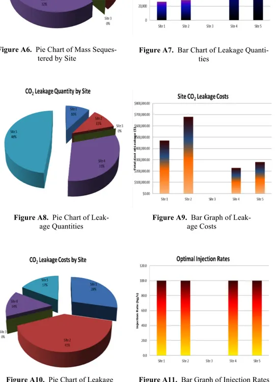
Figure A5 shows how much will be sequestered at any given time over the life of the project. This may be beneficial to project managers planning carbon capture schedules as well as monitoring projected vs. actual carbon storage. Figures A6-A12 graphically show the tabular data given in Figure 6.

(18)

Figure A6. Pie Chart of Mass

Seques-tered by Site Figure A7. Bar Chart of Leakage Quanti-ties

Figure A10. Pie Chart of Leakage

Costs

Figure A9. Bar Graph of

Leak-age Costs

Figure A8. Pie Chart of

Leak-age Quantities

(19)

Figure A12. Bar Graph of Injection