B
AIHETAN DISCHARGE TUNNEL
-U
SING
C
OMPUTATIONAL
F
LUID
D
YNAMICS
Carin Alderman & Sophia Andersson
© Carin Alderman & Sophia Andersson 2012
Degree Project for the master program in Water Systems Technology Department of Land and Water Resources Engineering
Royal Institute of Technology (KTH) SE-100 44 STOCKHOLM, Sweden
Reference to this publication should be written as: Alderman, C., Andersson, S., (2012). “Cavitation assessment of the Baihetan discharge tunnel – Using Computational Fluid Dynamics” TRITA-LWR Degree Project 12:13. 32 p.
The discharged water flows with a free water surface through the tunnel and has the characteristics of an open channel flow. Computational Fluid Dynamics (CFD) is used as a tool to retrieve the static pressures along the tunnel and to conduct a cavitation assessment of the structure.
Three different discharges– calibration, design and normal – are tested on the tunnel to see how the pressure is affected by varying flood situations. The results indicate three areas of interest where there is a risk of cavitation; these areas are located at the three existing disruptions of the bottom of the discharge tunnel. A slight difference in pressure between the discharges is observed, and cavitation will occur in all three cases.
Two major modifications of the tunnel are made in order to test the sensitivity of the results and to investigate what could be the ramifications due to construction errors or aging. These changes regard several variations of the tunnel bottom as well as altering the roughness height of the concrete lining. By changing the gradient of the tunnel at different locations the static pressure distribution is considerably affected, and in one case heavily reduces the risk of cavitation occurring in one of the troublesome locations. The changes made with regard to the roughness height barely alter the pressure distribution at all, and there is still a risk of cavitation at all of the three disruptions of the bottom.
The results of the CFD simulations are validated using recent cavitation theory as well as comparing the study to previous studies in the same area, and the values are found to be reasonable. Cavitation mitigation is recommended within the Baihetan tunnel to prevent heavy erosion. By aerating the water at the three disruptions of the tunnel bottom, the pressure of the fluid can be increased and thus prevent several severe damages to the structure. Since there is a lack of open channel flow research within the field of fluid dynamics, the results in this study can be used together with experimental data as a basis for future work in developing a system for confirming the accuracy of CFD simulations.
utskovstunnlarna från Baihetan-dammen för att utreda riskerna för kavitation i tunneln. Med hjälp av Computational Fluid Dynamics (CFD) modelleras vattenflödet för att ta reda på de statiska trycken längs tunneln och på så sätt kunna göra en sammanställning över kavitationsriskerna. Vattnet flödar med fri vattenyta genom tunneln och har samma egenskaper som öppen kanalströmning.
Tre olika flöden simuleras i tunneln för att undersöka hur trycket påverkas av vattenmängden. Dessa representerar det normala flödet, det dimensionerande flödet och kalibreringsflödet. För att undersöka hur känsliga resultaten är för eventuella konstruktionsfel görs två större modifikationer av tunnelns uppbyggnad. Dels testas flera variationer på tunnelns lutning, dels ändras råheten hos betongen på tunnelns yta. Resultaten visar att tre områden, alla tre placerade vid trappsteg i tunnelbotten, som löper speciellt stor risk att utveckla kavitation. Skillnaden i tryck mellan de tre fallen är liten, och kavitation kommer att uppstå vid samtliga flöden. En ändring av lutningen i tunnelns olika delar påverkar det statiska trycket i allra högsta grad - i ett fall minskas risken för kavitation avsevärt i ett av de riskfyllda områdena. Ändringen i råhet påverkar istället tryckfördelningen minimalt, och risken för att kavitation uppstår är fortfarande stor i alla tre områden.
Resultaten från CFD-analysen stämmer bra överens med både aktuell kavitationsteori och tidigare vetenskapligt arbete inom samma område, och värdena visar sig falla inom ett rimligt intervall. För att förhindra kraftig erosion i Baihetan-tunneln rekommenderas motverkande åtgärder. Genom att spruta in luft i vattnet vid de tre trappstegen i tunneln kan trycket i vätskan höjas och på så sätt förhindra skador på konstruktionen.
Då forskning om öppen kanalströmning inom flödesdynamiken är ringa skulle resultaten från denna studie kunna användas i framtida forskning tillsammans med provdata från modeller, för att utveckla ett system som kan bekräfta sannolikheten hos CFD-beräkningar.
高压力的强大射流。如果很多如此射流作用在同一表面,表面会开始侵蚀, 引起结构的巨大破坏。 该学位项目的目的是:为了确定是否存在空化的危险,深入研究白鹤滩泄洪 隧洞的泄流特性。在隧道中所泄水流的流动具有自由水面,具有一个明渠流 的特征,采用计算流体动力学的方法来获得沿隧道的静水压力的分布,并对 结构的空化进行评估。 对隧道的三种泄洪工况(校核、设计和正常泄洪工况)进行了测试,来看看 沿程压力如何随着泄洪的变化而变化。结果表明存在三个感兴趣的区域,那 儿存在着空化的危险;那些区域位于泄洪隧道底部三个突变的地方。在不同 泄洪量间仅存在着一个小的压力差,并且在所有三种工况都发生空化。 对隧道进行了二个主要的修改,其目的是为了测试结果的敏感性,以及研究 由于施工误差或结构老化可能产生什么后果。这些变动涉及数个隧道底部的 变化以及混凝土衬砌粗糙高度的变化。 通过改变在不同位置处的隧道底部的梯度,明显地改变了静水压力的分布, 在一种工况在三个不利位置中的一个空化产生的风险得到明显地降低。关于 粗糙高度的变更仅改变压力分布,但在三个底突变部位仍然存在着空化的风 险。 使用最近的空化理论以及对现在研究与同一领域中以前的研究进行了比较, 从而验证了 CFD 模拟结果,发现计算结果是合理的。建议了一些减轻白鹤滩 泄洪道产生空化的方式。通过对三个隧道底部突变区域内通气,可以提高流 体的压力,因此阻止几个严重的结构破坏。由于在流体动力学领域缺乏明渠 流的研究,可以使用本项研究及实验数据作为未来开发数值计算系统的基础, 以确认CFD 模拟的精度。
We owe our thanks to Dr. James Yang from Vattenfall R&D/KTH for making the trip possible and for all necessary arrangements. This project was funded by Elforsk AB within the frame of dam safety, where Mr. Cristian Andersson and Mrs. Sara Sandberg are program directors. Some funding was also obtained from KTH which enabled the accomplishment of the project.
Our supervisor Associate Professor Hans Bergh at the Department of Land and Water Research at Kungliga Tekniska Högskolan (KTH) was of great support to us, and we owe him our thanks and gratitude. Without his insights, this thesis would not be.
Last but not least we would like to thank our friends and families who supported us through the process and picked us up when our spirits were down.
Stockholm, February 2012
radiant/buoyancy [Pa/s] Slope gradient [-] Radiation intensity [-]
Kinetic energy per unit mass [J/kg] Pressure [Pa, bar]
Atmospheric pressure [Pa, bar] Critical pressure [Pa, bar] Vapour pressure [Pa, bar] Discharge [m3/s]
Entropy per unit mass [kJ/kgK]
Mass added to continuous phase from dispersed second phase [kg/(m3∙s)]
Source terms [-]
Time [s]
Temperature [°C, K]
Velocity/ Velocity vector/Component of velocity vector [m/s] Mean velocity/Fluctuating velocity [m/s]
Horizontal distance [m]
Depth [m]
Contribution of the fluctuating dilatation to dissipation rate [kg/(m∙s3]
Vertical distance [m] Volume fraction variable [-] Kronecker’s delta function1 [-] Turbulent dissipation rate [m2/s3]
Dynamic viscosity/Turbulent eddy viscosity [Pa∙s] Kinematic viscosity [m2/s]
Density [m3/s]
Cavitation index [-] Stress tensor [Pa]
Transferred heat per unit mass[W/kg]
Abstract ... 1
1. Introduction ... 1
1.1. Objectives ... 3
2. Theoretical background ... 4
2.1. Cavitation erosion ... 4
2.2. Computational Fluid Dynamics ... 7
3. Methods ... 11
3.1. Pre-processing ... 11
3.2. The solver stage ... 13
3.3. Post-processing ... 15
4. Results ... 17
4.1. The proposed tunnel design ... 19
4.2. Modifications of the tunnel ... 19
4.3. Velocity ... 24
4.4. Validation of the numerical model ... 24
5. Discussion ... 25
5.1. Method and accuracy ... 25
5.2. The proposed tunnel design ... 27
5.3. Modifications ... 28
5.4. Error assessment ... 29
6. Conclusion ... 29
References ... 31
Other references ... 32
Appendix A: CAD-drawing of the Baihetan discharge tunnel ... I
Appendix B: Geometry and mesh ... III
Appendix C: Ansys FLUENT settings ... VIII
Appendix D: Result of the static pressure ... X
The Baihetan dam is one of the largest hydro power projects in China at present. It has three discharge tunnels that all run the risk of developing cavitation damages. By modelling one of the tunnels using Computational Fluid Dynamics (CFD) it is possible to investigate where in the tunnel structure cavitation is likely to occur. This degree project assesses the risk of cavitation erosion in the Baihetan tunnel using the static pressure distribution, the velocity distribution and modern cavitation theory. Several modifications of the tunnel – including alterations in the gradient and construction parameters – are simulated in order to investigate if changes in the design can mitigate the cavitation problem. None of the analysed modifications completely eliminate the problem and aeration is recommended to counteract the problem. This study indicates where cavitation might be a problem in the Baihetan tunnel and can be used as a basis for further research.
Key words: Computational Fluid Dynamics (CFD); Discharge tunnel; Cavitation; Open channel flow; Static pressure; Baihetan hydropower project
1. I
NTRODUCTIONChinas fast growing economy in the past years has led to increased energy consumption in all levels of society. In order to fulfil this need, the Chinese government has decided to increase the national energy production with a special focus on renewable energy. The aim is to expand the production to 15% of the total usage of energy by 2020 with the main focus on development and expansion of hydropower. This decision has led to the construction of several new hydroelectric plants – mainly in western China. These new power plants are part of a project aiming to transfer available power from the west to the east where most of the energy is consumed (Ling, 2006).
In the construction of high dams in China, it has become increasingly common to build large-scale discharge tunnels (Han et al, 2008). These tunnels are normally used to handle excessive floods that cannot be discharged through spillways or bottom outlets (Zhang, 2011). One of the most important hydraulic parameters of a discharge tunnel is the design flood, due to the large flow rates discharged through the tunnel (Han et al, 2008). The high-velocity flow often produces a series of hydraulic problems in the tunnel due to the prevailing conditions of large discharges and high water heads (Canhua, 2001).
Discharge tunnels can be constructed in a large variety of ways, but generally the water first discharges through an intake orifice located near the bottom of the reservoir into a pressure tunnel. Water then arrives to a chamber where the operating gate is located (Han et al, 2008). The inlet gate controls the flow discharge and operates under high-pressure and high-velocity conditions (Mohagheg & Wu, 2010). This gate acts as the boundary between the pressure chamber and the free flow tunnel constructed on the other side. The free flow tunnel often consists of an upper section with a fairly straight slope, a parabolic section, a middle
section with a steeper slope, a bucket section and finally a ski-jump bucket outlet (Han et al, 2008). Stepped conduits constructed at the lower part of the tunnel have lately become the standard when designing a free flow tunnel as an alternative to a smoother design. The reason for this is the large difference in the maximum hydraulic load (Mohagheg & Wu, 2010). These steps can be employed as energy dissipaters, reducing the impact of the large flow on downstream constructions (Vischer & Hager, 1998). They are however subject to a suction that reduces the hydraulic pressure and induces the risk of cavitation occurring in the structure. This suction will increase with increasing velocities of the water flow (Mohagheg & Wu, 2010).
A relatively common way to reduce the costs of the construction of large-scale hydropower is to reuse diversion tunnels as discharge tunnels (Canhua, 2001). These tunnels are used during the construction stage of a dam to pass the flood flows (Plyushin & Gurtovnik, 1976).To be able to conduct this transformation, energy dissipaters have to be installed due to the high water head (Tian et al, 2009).
One of the largest on-going power projects is the construction of the Baihetan hydroelectric power plant and dam. It is located on the Jinsha River; a tributary of the Yangtze River in the provinces of Sichuan and Yunnan in south-western China (Fig. 1). The construction of the dam began in 2008 and is expected to be complete in 2019. The power station will have a total generating capacity of 13.05 GW produced through 18 turbines, each with a generating capacity of 725 MW. With this capacity the plant will be the third largest hydroelectric power plant in in the world after the Three Gorges Dam in China and Itapúa in Brazil. It will also be the fourth largest in the world in terms of reservoir volume and with a height of 289 m this double-arc concrete dam will be the third highest in the world as well (Zhang, 2011).
Baihetan will be able to handle a maximum discharge of 42 356 m3/s,
which can lead to critical problems in the spillways in aspect of energy dissipation and flood release. In the project the flood discharge problem has been solved by constructing six surface spillways, seven bottom outlets and three discharge tunnels. As water is discharged from the dam
Figure 1. Map over the Yangtze River showing the different on-going hydropower projects (Tian, 2009).
through the surface spillways and the bottom outlets, two horizontal layers of jets are formed that collides in the air; the energy then dissipates in the constructed basin in the narrow valley below (Fig. 2). By doing this the flow energy can be dissipated efficiently and have little impact on the different dam structures (Zhang, 2011).
A physical model of the Baihetan Dam with a scale of 1:100 has been built in the hydraulic laboratory of Tsinghua University in order to investigate the discharge capacity and the energy dissipation (Fig. 3). By using the model, an optimization of the design of the layout and the outlet structure could be proposed (Zhang, 2011). The model only studies the spillways and the bottom outlets and not the discharge tunnels.
One of the Baihetan discharge tunnels will have a total length of 2248.5 m and an arched roof where the internal height in the centre is 18 m throughout the geometry (Appendix A). The width of the tunnel is 15 m at the inlet and increases with 1 m after the second and third stepped conduit, to finally have a width of 17 m at the outlet. The gate chamber is situated at the beginning of the tunnel with a partly opened gate that divides the chamber from the upper section of the free water tunnel. The length of the upper part is 1873.56 m, with a gradient of
i=0.02. This is connected to the parabolic section which is curved
according to
The lower part of the tunnel includes three offsets, each with a height of 1.5 m. The length of this part is 245 m and has a gradient of i=0.25. The next unit is the bucket section which has a bucket radius of 300 m. The final part of the discharge tunnel is the ski-jump bucket outlet.
1.1. Objectives
The main purpose of this thesis is to assess the risk of cavitation occurring in one of the three discharge tunnels constructed at the
Figure 2. The Baihetan hydroelectric plant showing the two hori-zontal layers of jets and the constructed basin below (HHEC, 2011).
Baihetan hydroelectric plant. The high water head and the high-velocity flow in the tunnel increase the cavitation risk significantly, and can lead to hazardous erosion of the tunnel lining and underlying material. Computational Fluid Dynamics (CFD) modelling is used to investigate and analyse flow characteristics, such as the free water height, the velocity field and the pressure distribution along the tunnel bottom. Three types of flows were tested in the tunnel; the normal flow, the calibration flow (corresponding to a probability of 0.1%) and the design flow (corresponding to a probability of 0.01%). All flow through the tunnel with a free water surface. The sensitivity of the construction parameters where also tested by altering the tunnel design in the model. The result of this thesis can help conduct a rapid optimization of the structure design of the discharge tunnel and thereby improve the design efficiency.
2. T
HEORETICAL BACKGROUN DThis chapter describes the theoretical background on which the method, results and discussion in this thesis are based. The cause and impact of cavitation is discussed, with emphasis on what problems are likely to occur in spillways and possible mitigations. The equations governing turbulent fluid flow is presented together with the theoretical background to Computational Fluid Dynamics (CFD).
2.1. Cavitation erosion
All liquids have a vapour pressure, pv, which is dependent on temperature. If the temperature of the liquid is increased, the vapour pressure increases as well, up to the point where it assumes the same magnitude as the atmospheric pressure, p0. During this process, small bubbles containing the fluid in its gas phase start to grow in the liquid. When the atmospheric pressure is reached, the bubbles grow bigger until they collapse on themselves. This is the ordinary process of boiling (Khatsuria, 2005).
Another way for a liquid to boil is by lowering the surrounding pressures so that the liquid pressure is lesser than the vapour pressure in the
Figure 3. The physical model of the Baihetan surface spillways constructed at Tsinghua University 2011.
bubbles (Chow et. al., 1988). This phenomenon is called cavitation, and is defined as the breakdown of a liquid medium under very low pressures. The lowering of pressure typically forms at large turbulent pressure fluctuations (e.g. at turbines or fans), where local roughness of the wall produces wakes for cavities to develop in or where wall geometry creates local velocity acceleration of the fluid reducing the pressure (Franc & Michel, 2005). The most common places in a spillway for pressure decrease is at abrupt curvatures and where gate slots or similar constructions disrupt the smooth flow along a boundary (Fig. 4). The critical pressure for cavitation to occur is thus dependent on the temperature of the water. A lowering of the pressure can be present without causing cavitation if the deviation from the atmospheric pressure is smaller than the critical pressure, pc. The critical pressure is calculated as
In order to predict where cavitation has the possibility to appear or disappear, a parameter known as cavitation index (σ) is calculated. It is based on the Bernoulli equation:
Rearranging the Bernoulli equation gives the pressure coefficient Cp, also known as the Euler number.
The Euler number will remain constant along a body as long as the smallest pressure on the body is greater than the vapour pressure of the fluid. If the pressure drops to the minimum Euler number it will not decrease further, thus – using the vapour pressure – the upstream conditions corresponding to that critical pressure coefficient can be calculated and give a prediction of the extent of cavitation. This coefficient is called the cavitation index, σ.
Cavitation bubbles form and grow locally in areas where the pressure is far below the atmospheric pressure. As long as the pressure remains low the bubbles will not constitute a problem, but when the pressure increases again the bubbles cannot sustain their size and collapse on themselves. Each collapse creates a shockwave with the approximate velocity of the speed of sound in water (Fig. 5). The local pressure intensity at these infinitesimal shock areas is increased to about 200 times the local pressure. When many of these shockwaves act on the same
Figure 4. The formation of bubbles and location of erosion at non-uniformities in the spillway (Falvey, 1990).
place in a pipe, on a turbine or in a spillway, it causes erosion which in some cases can be very severe (Falvey, 1990).
2.1.1. Impacts
The extent of cavitation damage is dependent on the cavitation index, as well as the strength of the concrete surface. A cavitation index lower than 0.20 has been shown to cause considerable damage. In some cases, very deep pits (>10 m) have been discovered at the inspection of discharge tunnels and spillways. Nevertheless, minor damage might occur even if the cavitation index is higher. Usually, these minor damages are accounted for and are not considered important from a design point of view (Falvey, 1990).
Cavitation erosion is always found downstream of its source. When cavitation appears on a structure it will occur in similar locations elsewhere on the structure, making the targeting of additional damage control easy to position. Cavitation has many negative impacts on a system, and once cavitation damages occur it accelerates the rate of cavitation erosion. Some of the most severe impacts by cavitation on a system according to Khatsuria (2005) include:
Alterations in the performance of the system, usually to the worse
Appearance of additional forces not designed for on solid structures
Production of noise and vibrations
Erosion of the underlying material 2.1.2. Mitigation
Damage experience from the United States Department of the Interior (Falvey, 1990) show that cavitation damage on spillways become significant at water velocities exceeding 30 meters per second. Through small construction changes, the problem can be mitigated before any damages occur. The common mitigation method is aerating the water. Small quantities of air dispersed in the water have been shown to reduce the risk of cavitation erosion by increasing the surrounding pressure and preventing bubble growth. The quantity of air needed can vary between 3-10% of the total flow, and increases as the strength of the concrete in the spillway decreases. Several methods for aerating the water flow are presently in use. By changing the original construction, aeration can be performed without using energy-requiring mechanical pumps (Falvey, 1990).
Figure 5. The principle of bubble collapse causing cavitation erosion (Falvey, 1990).
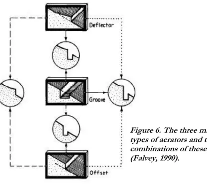
Three main groups of aerators are common; deflectors, grooves and offsets (Fig. 6). They can be used separate, but are often combined with each other. The function of the deflector is to lift the flow away from the boundary in order to allow aeration of the underside of the flow. If enough air is entrained in the flow, the resulting pressure will protect the downstream surface from cavitation erosion. Combining the deflector with a groove, offset or air duct in connection with the atmosphere is often essential for proper aeration of the flow (Falvey, 1990).
2.2. Computational Fluid Dynamics
Handling problems related to fluid flows have been a corner stone in the development of new technology during the 20th century, e.g. airplanes,
turbines and medical equipment. These flows often include turbulence and are thus difficult to describe and even more difficult to solve using simple calculation systems. With the development of computational power during the latter half of the 20th century, solving these problems
with the help of computers has to a greater extent been considered as an option. Today, Computational Fluid Dynamics (CFD) are a large part of the industry, with companies like General Electric and Boeing being frequent users, and numerous new models are initially designed and redesigned in the computer long before the first prototype is built (Hirsch, 2007). A lot of research has been associated with these applications, and the merits of CFD are well known. However, the use of CFD in open channel flows has hitherto been limited and little attention has been given to solution credibility for this area (Hardy et al, 2003).
2.2.1. Background
The non-linear partial differential equations that describe the behaviour of turbulent fluid flows are called the Navier-Stokes equations and are derived from applying Newton’s second law on fluid motion. In order for the equations to be valid the flow has to be continuous, and the conservation of mass, motion and energy within the fluid are essential when setting up the equations (Hirsch, 2007).
Figure 6. The three main types of aerators and the combinations of these (Falvey, 1990).
Conservation of mass is the first equation in the system and is described as
The second equation set up in the Navier-Stokes system is the conservation of momentum (motion) and is described as
Where the stress tensor is
The third equation is the energy equation, which governs the conservation of energy in a fluid flow.
The energy equation is only employed if the temperature is of interest or governs the flow in some way. If the temperature of the flow can be considered constant, the energy equation can be excluded (Hirsch, 2007). 2.2.2. Pre-processing
In the pre-processing stage, the studied structure is transformed into a computable model using pre-processing software. This software is often compatible with modern CAD-software, but has the option of altering designs or even building the complete structure within the program itself. Both 2D and 3D models can be generated, complete with mesh and boundary conditions (FLUENT, 2000).
The first step of the discretization process is to transform the drawings of the system into a computer model. The extent of the model in space is important and has to be taken into consideration when building the model. In order to reduce the number of calculations, justifiable simplifications of the model, e.g. symmetrical links or generalizations of the geometry that will not affect the outcome, can be made (Hirsch, 2007).
The resulting geometry is meshed. Meshing is the process of dividing the model into many small control volumes, or cells, that are used for the calculations in a solver. The mesh can be structured or unstructured. In 2-dimensional space, an unstructured mesh is represented by triangular
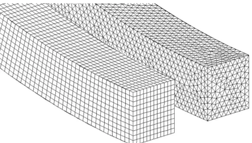
Figure 7. Showing the difference between applying a structured (right) and an un-structured (left) mesh at the outlet of the Baihetan tunnel.
proper unstructured mesh without user interaction. This is because unstructured meshes are far easier to fit to complicated geometries, but the arbitrary number of neighbouring cells demands a lot of computational power. The difficulties of aligning the cells with the flow direction lead to false diffusion –a numerical error not represented by a physical phenomenon. Therefore, the aim is to achieve a structured mesh whenever possible (Blazek, 2002).
The density of the mesh is of high importance and will affect the final result. The mesh size should thus be determined by the desired level of accuracy. Other aspects to consider are the computational power available and the extent of the model in time and space. If computational power is low, refining the mesh just at the critical locations (e.g. close to boundaries) in the model can be an option (FLUENT, 2000).
The final step of the pre-processing is assigning boundary conditions to the model. Boundary conditions specify flow and thermal variables at the boundaries of the physical model and are essential in creating an appropriate model for turbulence simulations (FLUENT, 2000).
2.2.3. Solver
Turbulence is the time-dependent chaotic behaviour seen in most fluid flows. Although the problem is universal and has applications in many different fields, it has not yet been proven that the Navier-Stokes equations have three-dimensional solutions that do not contain any one singularity and thus describe the problem accurately. Still, the Navier-Stokes equations provide the best solution currently available and are therefore widely used as the basis for turbulence problems (Hirsch, 2007).
There are many solvers on the market that deal with turbulence problems. The final mesh from the pre-processing stage is imported into the solver and the flow parameters are set in the program in order to give as accurate a description of reality as possible. However, turbulence problems tend to be very complicated and require an extremely fine mesh in order to produce a stable solution, to the point that computational power is insufficient or unobtainable (Hirsch, 2007). Laminar solvers use considerably less computer power, but usually fail to converge when dealing with turbulence. To counter this problem, time-averaged equations like the Reynolds-time-averaged Navier-Stokes equations (RANS) are used in CFD (FLUENT, 2006).
The idea behind RANS is the Reynolds decomposition, where a time-dependant quantity is decomposed into its average and fluctuating value at any instant, in the form
, where
When applied on the Navier-Stokes equations they give an approximate solution to otherwise near-impossible problems. The momentum equation will be given the following appearance:
Integration in time removes the time dependence of the resultant term and the momentum can then be calculated as
The velocity fluctuations due to the inertia of the fluid are the source of eddies in a turbulent flow and the physical manifestation of turbulence kinetic energy (TKE). In order to accurately calculate the TKE, the flow field has to be discretized as far as the Kolmogorov micro scales2 –
which require too much computer power to be realistic. To cope with this problem, there are many simplified turbulence models in use; such as the RANS k-ε model, the RANS k-ω model and the large eddy simulation (LES) model. The most common model used is the k-ε model, which is a two-equation model that assumes isotropy of turbulence, resulting in equal normal stresses. Its popularity is mostly due to its usefulness in a wide range of turbulence problems (FLUENT, 2006).
The turbulence kinetic energy and its dissipation (denoted k and ε, respectively) can be calculated using two transport equations:
Relating the RANS stresses to the mean velocity gradients is in the k-ε model commonly done by means of the Boussinesq hypothesis3. This
approach reduces the computational costs associated with calculating the turbulent viscosity, μt, as a function of k and ε.
A large number of flows encountered in fluid problems consist of multiple phases flowing together, e.g. water and air, water and oil, ink and air etc. It is thus important to choose a multiphase model for the calculations. One such model is the volume of fluids (VOF) model first published by Hirt & Nichols (1981). The model can be used on two or more phases when the intersection between the phases is of interest. VOF proposes that the phases never interpenetrate and tracks the content of a phase in each cell throughout the domain. For the qth phase,
the continuity equation for the fraction of that phase is
2 In 1941, Andrey Kolmogorov introduced the idea that the smallest scales of turbulence depend only on ε and ν and are similar for every turbulent 3 Boussinesq’s hypothesis from 1877 assumes that eddy turbulence can be modeled using a scalar μt for eddy viscosity (FLUENT, 2006).
2.2.4. Post-processing
The Navier-Stokes equations dictate velocity rather than position, and the solution consists of a velocity or flow field. These solutions can be shown directly by the solver in the form of graphs, tables or animations. The interpretation then rests on the user. If needed, the parameters sought can be exported for further computations in other software. 2.2.5. Model validation
Difficulties regarding solution credibility when modelling open channel flows are discussed by Hardy et al (2003). They pointed out that while a lot of research has gone into discretizing and solving the RANS-equations, little attention has been given to developing a definite way of verifying and validating the 2D or 3D model. They developed a technique called Grid Convergence Index (GCI) as a way of determining if a proposed grid would provide accurate results, but concluded that depending on the variable measured, the GCI could verify and disprove a grid simultaneously.
An alternate way of validating a CFD model is by comparing it with experimental data from physical model tests. This was done by for instance Axelsson & Knutsson (2011) and Margeirsson (2007). Both studies concluded that CFD modelling of a spillway has some merits, but that it can differ a lot in singular points and that further studies are needed.
3. M
ETHODSThe different steps conducted during this study are presented in this section. The pre-processing was carried out before any calculations could be performed. During this step a model of the discharge tunnel was produced in GAMBIT 2.3.16. This software generated the geometry, the mesh and provided the model with boundary conditions. GAMBIT is the pre-processing software associated with Ansys FLUENT, into which the final model was imported. FLUENT 6.3 was used both as the solver program and as a part of the post-processing combined with Microsoft Excel.
3.1. Pre-processing
The geometry of the discharge tunnel was created using information from a CAD-drawing (Appendix A) provided by Associate Professor Li Ling (2011). Due to the uncertainty of the water surface’s symmetrical behaviour in the tunnel, a 3-dimensional model was desirable in order to correspond better with reality.
To make further calculations in the solver stage easier, several simplifications were carried out regarding the geometry of the tunnel. Both the gate chamber at the inlet and the ski jump bucket outlet were completely removed from the model, since they were not of interest in the assessment. These simplifications caused the model to stretch from 17.88 m to 2248.5 m in the horizontal direction (x) and from 650 m to 787.65 m in the vertical direction (z) (Appendix B).
It was also assumed that the shape of the ceiling of the tunnel would have little effect on the static pressures since only the primary phase would exist here at all times during the calculations. Considering this, and to reduce the difficulties of meshing, the arched roof of the tunnel was altered into a rectangular one with a constant height of 18 m.
3.1.1. Establishing the mesh
When computing a complex three-dimensional model it is essential to optimize the total number of cells in the meshing stage. The computer capacity significantly limits the amount of cells practical to use, but with a decreasing number of cells the accuracy of the final result reduces. By devoting time at the beginning of the solver stage to establish the optimal number of cells for the desired calculations, the computing time used in further analysis can be heavily reduced.
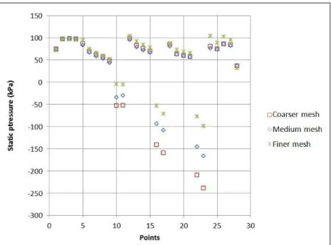
To determine the optimal number of cells for the calculations in this research, three different cases with identical geometry were studied to see how their differences would affect the end results. Three meshes with different intensities were created (Table 1). All meshes were generated in a structured grid to save computational power and avoid false diffusion complications associated with turbulence. These cases were imported into FLUENT to compare the static pressure distribution along the bottom of the tunnel (Fig. 8).
Accuracy, time frame and computational power are all important factors to consider when choosing a final mesh. The time frame of the project determined how much time could be devoted to calculations and naturally the best accuracy possible was sought. Due to lack of computational power, but with the ambition of producing the most accurate results possible, the medium sized mesh of case 2 was chosen
Table 1. The amount of cells for each case
Case Mesh Number of cells
1 Coarse mesh (4x20 meters) 2 632
2 Medium coarse mesh (2x10 meters) 17 566
3 Finer mesh (1x5 meters) 125 875
Figure 8. The static pressure distribution for the different mesh cases.
3.2.1. FLUENT settings
A steady state solution was enabled as recommended by FLUENT (2006) when modelling open channel flows. Since cavitation erosion is the result of long term exposure to below-atmospheric pressures, the intermediate flow between the initial water flow in the tunnel and the stabilized flow is of little interest.
The volume of fluid (VOF)-scheme with two phases, one primary and one secondary, was chosen as the multiphase model in accordance with FLUENT (2006). The primary phase was defined as air and the secondary as liquid water, using the material attributes provided by the software. The parameters of VOF enabled were the open-channel flow and the implicit scheme. By enabling implicit body force the solution will be more robust and converge faster. This application also takes into account the equilibrium between the body force in the momentum equation and the pressure gradient. The energy equation was disabled since the temperature was not of interest and the force of the energy was negligible compared to the other acting forces.
The model chosen for the viscous model was the standard RANS k-ε model, since it is the most common model used for these types of cases and requires less computational effort in comparison with other k-ε models. The operating pressure of the calculations was defined as the atmospheric pressure and the location of the reference pressure was placed at the top of the inlet, since at no point during the calculation process will the secondary phase occur at this spot. In addition, gravity was activated since it is recommended when modelling an open channel flow. The specific operating density was set to 1.225 kg/m3, the
density of air at normal temperatures, which is the density of the lightest phase.
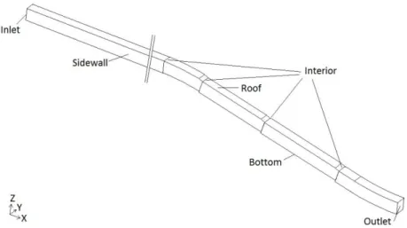
Figure 9. The Baihetan tunnel (cropped) with the names of the boundaries assigned in GAMBIT.
The model imported from the pre-processer had been assigned general conditions for each boundary, but the specific settings were defined in the solver (Table 2). The upstream conditions of the dam regulate how much water will be released through the tunnel, and three flow rates were considered in the calculations. The flow rates correspond to an initial free water surface level in the tunnel and determine the mass flow rate used as specific settings for the mass flow inlet (Table 3). All other settings remained the same for all flow rates.
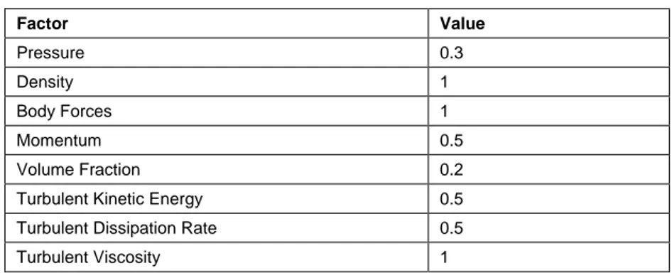
FLUENT uses different algorithms for its calculations. The chosen algorithm for the pressure-velocity coupling was SIMPLE, since it handles turbulence with good precision and is recommended for steady state flows (FLUENT, 2006). PRESTO! was selected for the pressure discretization and Modified HRIC (High Resolution Interface Capturing) was enabled for the volume fraction because it improves the accuracy of the VOF calculations. The first order upwind discretization was set for the momentum, the turbulent kinetic energy and the dissipation rate. The setting was chosen due to lack of computer power, nonetheless the discretization gives a better convergence than the second order upwind, but it gives less accurate results.
3.2.2. Monitoring of convergence
An absolute criterion for the residuals was set to evaluate whether the solution reached convergence or not. For the solution to be considered converged all the residuals had to be less than 10-3. In order to force the
solution to converge the under-relaxation factors were reduced to a lower value than their default ones (Table 4). Another way to monitor the calculations is to examine the flux report; it shows the balance between the overall mass, momentum, energy and scalar balances. When the imbalance of the flux is less than 0.2% the solution has converged. The solution can also be considered converged when the result does not change with more iteration (FLUENT, 2006).
Table 2. Boundaries and settings in FLUENT
Boundary name Boundary type Phase Settings
Bottom Wall Mixture Roughness height = 0.003 m Inlet Mass Flow Inlet Mixture Open Channel
Free surface level = * m Bottom level = 769.64 m Air Mass flow rate = * kg/s Water Mass flow rate = * kg/s
Interior Interior - -
Outlet Pressure Outlet - -
Roof Pressure Inlet - -
Sidewall Wall Mixture Roughness height = 0.003 m
*See Table 3 for the specific setting.
Table 3. Discharge capacities with corresponding flow details
Normal Q=3789.3 m3/s Calibration Q=3905.8 m3/s (P=0.1%) Design Q=4083.0 m3/s (P=0.01%)
Inlet Free surface level 778.64 m 778.75 m 779.14 m
Mass flow rate (air)
3 174 kg/s 3 203 kg/s 3 108 kg/s Mass flow rate
(water)
Turbulent Dissipation Rate 0.5
Turbulent Viscosity 1
3.2.3. Modifications of the tunnel
When constructing a discharge tunnel of the same magnitude as the Baihetan tunnel, some minor or major construction errors are probable to occur. A small miscalculation may lead to a flatter or steeper slope than originally intended. Some material parameters, such as the roughness of the lining concrete, also change with age and usage (Falvey, 1990). When these types of incidents occur, it could increase or decrease the risk of cavitation erosion. To investigate this risk, small modifications of the geometry and the construction parameters were made in the model. All modifications were calculated for and compared with the normal flow rate, Q = 3789.3 m3/s.
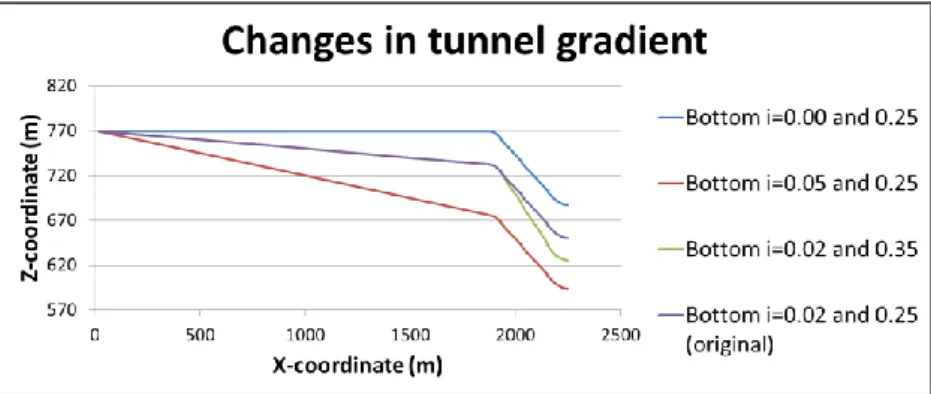
To monitor how a gradient change would affect the flow characteristics, the tunnel was divided into three parts; before the bend, the bend itself and after the bend (Fig. 10), and three conditions were created where one part of the tunnel differed from the original slope. Condition 1 and 2 were given two completely different gradients before the bend, but both had the same gradient as the original condition after the bend. In condition 3 the slope gradient after the bend was altered instead, but kept unaltered before the bend (Table 5, Fig. 11).
The second modification was an alteration of the roughness height of the walls. This parameter is dependent on the features of the concrete lining used on the tunnel surfaces. Two additional conditions were tested apart from the original condition, one lower and one higher (Table 6). Both conditions are within reasonable values for concrete lining (Bergh, 2011; Chen et. al., 2010).
3.3. Post-processing
In the post-processing stage the calculations made by the solver were treated and analysed. Both FLUENT and Microsoft Excel was used in the acquiring and presentation of the results.
Figure 10. The three parts of the Baihetan tunnel, 1=before the bend, 2=the bend, 3=after the bend.
3.3.1. Static Pressure Distribution
In order to determine where cavitation might occur, the pressure distribution along the bottom of the tunnel had to be established. This was done by manually allocating a number of carefully selected points along the bottom to monitor the pressure. The points represent areas of special interest as well as an evenly spread distribution along the boundary. The total number of points was determined to be 28 (Appendix D) and the value of the static pressure at each point was obtained and plotted.
3.3.2. Velocity
Another of the characteristics investigated was the velocity throughout the tunnel. Examining the velocity will make it easier to understand the relationship between the velocity and the pressure. The velocity also affects the impact caused by cavitation.
Table 5. Modifications made to the slope of the tunnel
Condition Slope before the bend Slope after the bend
Original i=0.02 i=0.25
1 i=0.00 i=0.25
2 i=0.05 i=0.25
3 i=0.02 i=0.35
Table 6. Modifications of the roughness height
Condition Roughness height
Original 0.003 m
1 0.001 m
2 0.005 m
Table 7. A compilation of the different CFD simulations tested
Discharge Type Slope Roughness height
Q=4083.0 m3/s Original cases i=0.02 and 0.25 k=0.003 m Q=3905.8 m3/s i=0.02 and 0.25 k=0.003 m Q=3789.3 m3/s i=0.02 and 0.25 k=0.003 m Gradient modifications i=0.00 and 0.25 k=0.003 m i=0.05 and 0.25 k=0.003 m i=0.02 and 0.35 k=0.003 m Roughness modifications i=0.02 and 0.25 k=0.001 m i=0.02 and 0.25 k=0.005 m
Figure 11. The four different modifications made to the slope in relation to each other.
Figure 12. Pressure level along the whole tunnel for all three discharges.
Figure 14. (a) top – Pressure difference at all three offsets along the tunnel bottom for a discharge of 3 789.3 m3/s.
(b) middle – Pressure difference at all three offsets along the tunnel bottom for a discharge of 3 905.8 m3/s.
(c) bottom – Pressure difference at all three offsets along the tunnel bottom for a discharge of 4 083 m3/s.
The static pressure distribution along the bottom of the tunnel was sought since areas of lower than atmospheric pressure run the risk of developing cavitation damages. The value of the static pressure was related to the atmospheric pressure at 28 points along the tunnel bottom, showing pressures below atmospheric pressure as negative (Fig. 12). Because of the three-dimensional extent of the model, the central y-axis was considered representative for the pressure distribution, and all points were located along this axis.
A closer examination of the pressure levels in the upper part of the tunnel reveals that the pressure increases gradually along the bottom until the bend, where it starts to drop. Three areas of interest emerge from analysis because they differ from the remainder of the pressure results (Fig. 13). These all occur at the same locations – at each offset of the bottom – for all of the flow conditions. In these areas, the static pressure decreases to a negative value and increases again almost directly until it reaches a fairly constant positive pressure. The decrease in pressure in the three areas is greater with each offset along the tunnel bottom for all of the flow conditions (Fig. 14a-c). It can also be noticed that the pressure drops to a lower positive value at the outlet of the discharge tunnel.
With a higher discharge the static pressure increases in all points making the negative values less negative and the pressure difference at each drop decreases. All the values of the statistic pressure at each point can be seen in the appendices.
4.2. Modifications of the tunnel
Two different types of modifications were made on the tunnel model. The first was the change in gradient at different sections of the tunnel, which resulted in three different conditions. The second modification studied was a presumed change in roughness height.
Figure 16. (a) top – Static pressure difference between the three changes in gradient at the first offset in the tunnel.
(b) middle – Static pressure difference between the three changes in gradient at the second offset in the tunnel.
(c) bottom – Static pressure difference between the three changes in gradient at the third offset in the tunnel.
For the second condition with a gradient of i = 0.05 in the first part the result shows that all of the three interest areas have negative static pressures (Fig. 17). This modification gives a higher pressure difference at all of the three offsets (Fig. 16a-c).
In the third condition the modification was made in the third part of the tunnel, where the slope was set to i = 0.35 (Fig. 18). From the pressure distribution it can be noted that the pressure difference in the third offset is affected more than in the other offsets; the difference is almost as high as for the second condition (Fig. 16c).
Figure 17. Pressure level along the tunnel bottom with an increased gradient of
i=0.05 in the first part of the tunnel.
4.2.2. Modification of roughness height
With a change in surface roughness the results show that the same three areas – the offsets - are subjected to negative pressures in both the conditions (Fig. 19). The difference in pressure between the cases does not alter significantly (Fig. 20).
By lowering the roughness height to 0.001 meters, the pressure decreases in all points except at the outlet where a small increase occurs. The negative values are affected more than the positive and decreases significantly. Increasing the roughness height to 0.005 meters reverses this effect, i.e. the static pressure increases at all points with the exception of the outlet where it decreases. With the higher roughness height the negative pressures are shown to be less negative and the pressure difference is decreased (Fig. 21a-c).
Figure 19. Pressure level along the whole tunnel for all three roughness heights.
Figure 20. Pressure level along the lower part of the tunnel for all three roughness heights.
Figure 21. (a) top – Pressure difference at the first offset for all three roughness heights.
(b) middle – Pressure difference at the second offset for all three roughness heights.
(c) bottom – Pressure difference at the third offset for all three roughness heights.
4.3. Velocity
A continuous field was used to illustrate the velocity throughout the tunnel. To investigate how much the velocity influences the pressure, it is interesting to compare the cases that have the greatest pressure difference. These cases are the normal flow and the three gradient modifications, all with an inlet velocity of 28 m/s. In the original condition, the velocity increases with each offset and the highest velocities occur in the central cross-section of the flow (Fig. 22). Examining condition 1 shows an overall decrease in the velocity throughout the tunnel compared to the original condition, but especially in the first section of the tunnel (Fig. 23). In condition 2 the velocity increases in the entire tunnel (Fig. 24), while in condition 3 the velocity only increases after the second offset (Fig. 25). The maximum and minimum velocity for the entire tunnel was extracted for each condition (Table 8), revealing that condition 2 has the highest maximum velocity and condition 1 the lowest. The widening of the tunnel –at the second and the third offset – displays low velocities at the downstream side walls of the offsets, nevertheless the velocity in the middle of the tunnel will still be high.
4.4. Validation of the numerical model
Comparing the numerical data to some form of experimental data is a common way of conducting model validation for dam structure models. Since no experimental data exist for the Baihetan tunnel, other measures had to be taken to ensure that the computational results are valid. The GCI technique was dismissed, since it has not been proven to be of universal applications and not all required parameters where known. Instead, investigating the model according to cavitation theory was used for locating vulnerable places in the tunnel. Cavitation typically forms at disruptions of a smooth boundary, suggesting that the three offsets found in the Baihetan tunnel can be problematic areas (shown as B in fig. 4). The bend could also be of interest, since sharp curvatures also can be subject to cavitation (shown as C in fig. 4). Another way to indicate where cavitation may occur is the cavitation index. By calculating the cavitation index (Fig. 26) for all 28 pressure points along the bottom, potentially problematic areas could be identified as having an index value lower than 0.20 (Appendix E).
The result was also compared with a similar study made by Axelsson and Knutsson (2011). They modelled a spillway system using CFD to investigate the discharge capacity, the pressure distribution along the
conclusion was that CFD produces realistic values for the pressure distribution, but that the deviation from scale models can, in complex geometries, be greater than desired. The calculations were conducted using the same software and all major settings were the same in both studies, which suggest that similar problems can be present in the Baihetan study.
5. D
ISCUSSIONThe results of the CFD simulations employed in this degree project were compared with theories presented in previous research and were shown to agree with the expectations of an open channel flow. The following section discusses in detail both the original model and the modifications made, along with evaluation of the CFD method and possible sources of error.
All of the results showed that negative pressures will occur downstream of the offsets. Depending on the magnitude of these pressures, they could be potentially harmful. To determine whether a specific negative pressure can generate cavitation, the critical pressure is of interest. The temperature of water determines the vapour pressure which in turn determines if cavitation will occur. An assumption of the water temperature being 10°C in the discharge tunnel will lead to the water vaporizing if the pressure drops to 1 kPa or less. The critical pressure will then be pc = -10 kPa if the atmospheric pressure is assumed to be 101.3 kPa. A lower water temperature will decrease the critical pressure, while a higher temperature places the critical cavitation point closer to the atmospheric pressure.
5.1. Method and accuracy
The widespread use of CFD in the industry by companies such as Boeing and General Electric shows that the method has respectable credibility among the very top experts in their respective field and that has a variety of applications where it has been proven to produce accurate results. The use of CFD in open channel flows has not been as thoroughly researched as it has for other fields and therefore there is no validation method of universal application. Even so, there are still ways of confirming the results from the CFD; e.g. by completing it with experimental data. The Shibuya study by Axelsson and Knutsson (2011) shows that even though the numerical model seems to have an internal logic, the pressure difference in a single point can still be almost 600% between the scale model and the numerical model. The problem with CFD is not the equations, since the Navier-Stokes system is valid for all flows. Instead, more research regarding settings and algorithms used for open channel flow is needed. Hopefully, in the near future CFD simulations can be carried out without completing it with other research in order to ensure compliance with reality
Figure 23. Velocity field of the lower section of the tunnel, with a decreased gradient to i=0.00 in the upper part of the tunnel and a discharge of Q=3 789.3 m3/s.
Figure 24. Velocity field of the lower section of the tunnel, with an increased gra-dient to i=0.05 in the upper part of the tunnel and a discharge of Q=3 789.3 m3/s.
Figure 25. Velocity field of the lower section of the tunnel, with an increased gra-dient to i=0.35 in the last part of the tunnel and a discharge of Q=3 789.3 m3/s.
A specific problem present in this study is the occurrence of impossible pressure values in the CFD calculations. All pressures within the model were referred to the atmospheric pressure, giving pressures below atmospheric pressure as negative pressure. The atmospheric pressure is 101.3 kPa, making 0 Pa the approximate value of -101.3 kPa in the model. Some of the results are lower than this value, some even twice as low. Since this is a factual error that the solver does not take into account, these values have been used as an indication of where cavitation will occur, but their individual values have not been considered reasonable.
CFD is still a valid method for many turbulent fluid flow problems. The technique enables calculations to be performed on a more complex and larger scale, and allows easy modification of the numerical model. Additionally, in this study, the indication of low pressure areas is considered more important than the actual values, and therefore the fact that some pressures may not be exact is of little interest.
The accuracy of a model generated by the CFD method is also dependent on the computational power. It will determine how many calculations can be performed per time unit and thus, how many cells the mesh can consist of without increasing the calculation time to unacceptable values. With a higher capacity at hand, the researcher can also impel the solver software to generate a better and a more precise result since a wider range of settings can be applied in the solver stage. In this study, the lack of computational power limited the optimization of the amount of cells used in the model mesh, which led to a relatively coarse mesh being used for the calculations. Using a denser mesh would have resulted in each simulation taking as long as 24 hours or more to perform and prolonging the study with several months. If more advanced computers had been available, the result might have been more accurate in terms of the actual values.
5.2. The proposed tunnel design
When plotting the static pressure along the tunnel bottom, three different areas were detected that could be of interest when investigating the cavitation risk of the Baihetan discharge tunnel. The modelling showed that these areas had a significant drop of pressure in all cases.
The three areas are all situated at disruptions of the smooth boundary, both along the tunnel bottom and - in the two downstream areas - along the wall. Cavitation theory suggests that these locations will be troublesome, which is confirmed by the CFD results. All three areas have a cavitation index of <0.2 and display pressures below the critical value, which would suggest that cavitation is a serious risk here. Cavitation erosion will invariably occur once the pressure increases again, threatening the structure of the tunnel bottom and walls.
The maximum velocity in the tunnel for all the conditions exceeds the limit of 30 m/s. This indicates that there is a significant risk for more severe impacts on the structure which will become higher at each offset due to an increasing velocity.
The flows investigated represent three floods with a probability of occurrence of 0.01%, 0.1% and a normal flood situation. Since a greater water depth increases the hydrostatic pressure (assuming the fluid is incompressible), it is only to be expected that the pressure increases in all points along the bottom as the flow rate – and thus the initial water level – increases, but the pressure still drops below the critical point in all three areas. The normal flood should be considered to have the greatest risk of cavitation – both because it has the lowest pressures and because it is most likely to occur.
The simplifications made prior to the discretization are thought to have little influence on the final results. The inlet pressures are within the expected range, suggesting that the removal of the inlet gate has little effect on the calculations. At the outlet, where the ski-jump bucket was removed, the pressure changes suddenly in several of the cases. This change is notable but small, and it does not cause any cavitation risk in the area. Therefore, this simplification is considered justified for all conditions. By changing the shape of the roof, and thus increasing the area available for air flow, it is possible that the pressures are affected all through the tunnel. This would be a systematic error that is hard to discover without comparing the results to experimental data. It is assumed that such an error would be proportional throughout the model. Since the focus in this study is on cavitation risk rather than on absolute pressures, the potential errors this could cause is thought to be of little importance to the conclusions.
5.3. Modifications
The modifications were made to investigate what could happen if the construction should change in any way. However, the natural level difference between the reservoir and the downstream basin will govern how much the tunnel has to slope and some of these modifications may not be relevant. The idea of the modification was to function more as a sensitivity check rather than as modifications that could be carried out in reality.
The modifications made in aspects of gradient change at different parts of the discharge tunnel affected the static pressure in different ways depending on where the change was made. A decrease in tunnel gradient as for the first condition slows down the velocity of the water (Fig. 23), increasing the pressure in all points. The initially higher pressure before the bend causes the pressure at the first offset to stay positive, even though the pressure difference is almost as high as for the other conditions. The second and third offsets still have pressures below the critical point and will develop cavitation. Consequently, an increase in tunnel gradient in condition 2 and 3 has the reversed effect. The velocity
affect the pressure significantly and cavitation will still occur at the same three areas. A decreased roughness height reduces the friction of the tunnel surface and thus increases the velocity that in turn decreases the pressure. The reversed effect occurs when the roughness height is increased. Due to the small change in pressure, the concrete chosen initially for the surfaces in the tunnel is not of major importance concerning improvement of the structure to prevent cavitation. An aging concrete will with high probability slightly reduce the problem rather than increasing it, since a rougher surface increases the static pressure. However, concrete may weaken with time and erode easier, thus making the situation worse. This aspect has not been further examined since it does not fall under the scope of this thesis.
5.4. Error assessment
There are many potential errors in the simulations that need to be addressed in order to determine if the modelling can be assumed probable or not. Simplifying the geometry of the discharge tunnel could affect the static pressures more than intended, and possibly more than is realistic. This has not been taken into account when setting up the model. The definition of the boundary conditions in the pre-processor and their individual settings in the solver may have been the result of erroneous assumptions, although this risk is bigger for the specific settings than for the choice of boundary conditions. Other settings in the solver stage, although set using the recommendations by FLUENT (2006), could prove to be unsuitable for this particular problem.
6. C
ONCLUSIONPrevious experiences from other studies regarding cavitation suggest that offsets such as the three existing ones in the Baihetan discharge tunnel are areas with a high risk of cavitation. These three steps in the tunnel disrupt the smooth flow boundary of the spillway and will be subjected to decreased pressures which will generate cavitation bubbles. The CFD simulations and cavitation calculations carried out in this thesis all confirm this. The question is whether these bubbles would be able to damage the structure or not, i.e. if the pressure would drop below the critical vapour pressure of the water. In all of the cases and modifications this has been revealed to be highly likely at all offsets (with one exception), and aeration mitigation is recommended to reduce or prevent the impact of cavitation on the structure.
The three flows simulated in the tunnel represented possible flood situations that the tunnel is designed to handle. The normal flow proved to be the most likely to develop cavitation since it had the lowest static pressures. Although the risk is somewhat reduced for the calibration and design flows it is not completely eliminated, and cavitation is still a major concern during all flood events.