2003:30 Research and Development Program in Reactor Diagnostics and Monitoring with Neutron Noise Methods

SKI Report 2003:30

Research

Research and Development Program in

Reactor Diagnostics and Monitoring with

Neutron Noise Methods

Stage 9. Final Report

I. Pázsit

V. Arzhanov

A. Nordlund

D. Olsson

SKI Perspective

How this project has contributed to SKI’s research goals The overall goals for SKI research are:

• to give a basis for SKI ’s supervision

• to maintain and develop the competence and research capacity within areas which are important to reactor safety

• to contribute directly to the Swedish safety work.

Above all, this project has contributed to the strategical research goal of competence and research capacity by building up competence within the

Department of Reactor Physics at Chalmers University of Technology regarding reactor physics, reactor dynamics and noise diagnostics.

The project has also contributed to the research goal of giving a basis for SKI’s supervision by developing methods for identification and localization of

perturbations in reactor cores. Such an example is the development of a detector (the so-coalled Cf-252) for measurement of the reactivity in subcritical cores. The report comprises stage 9 of a long-term research and development program. The results have been published in international journals and have been included in both licentiate- and doctor’s degrees.

Project information:

Project manager: Ninos Garis, Department of Reactor Technology, SKI

Project number: 14.5-020984-02274

Previous reports: SKI report 95:14 (1995), 96:50 (1996),

97:31 (1997), 98:25 (1998), 99:33 (1999), 00:28 (2000), 01:27 (2001), 2003:08 (2003).

SKI Report 2003:30

Research

Research and Development Program in

Reactor Diagnostics and Monitoring with

Neutron Noise Methods

Stage 9. Final Report

I. Pázsit

V. Arzhanov

A. Nordlund

D. Olsson

Department of Reactor Physics

Chalmers University of Technology

SE-412 96 Gothenburg

Sweden

September 2003

This report concerns a study which has been conducted for the Swedish Nuclear Power Inspectorate (SKI). The conclusions and viewpoints presented in the report are those of the author/authors and do not

Research and Development Program in Reactor Diagnostics

and Monitoring with Neutron Noise Methods: Stage 9

Summary

This report gives an account of the work performed by the Department of Reactor Physics, Chalmers University of Technology, in the frame of a research contract with the Swedish Nuclear Power Inspectorate (SKI), contract No. 14.5-020984-02274. The present report is based on work performed by Vasiliy Arzhanov, Anders Nordlund, Dan Olsson and Imre Pázsit, with the latter being the project leader.

This report constitutes Stage 9 of a long-term research and development program concerning the development of diagnostics and monitoring methods for nuclear reactors. The long-term goals are elaborated in more detail in e.g. the Final Reports of stage 1 and 2 (SKI Rapport 95:14 and 96:50, Refs. [1] and [2]). Results up to stage 8 were reported in [1] - [8]. A brief proposal for the continuation of this program in stage 10 is also given at the end of the report.

The program executed in Stage 9 consists of four parts and the work performed in each part is summarized below.

Development of reactor kinetics and dynamics for systems with non-stationary boundaries

Studies of the space-time dependent neutron flux in systems with a non-constant volume, i.e. having time-dependent boundaries, have been already started at the Department. They were motivated by the need of calculating the neutron noise induced by vibrating control rods and core barrel vibrations. A general formalism was developed in the frame of linear noise theory in the one-group approximation and homogenous bare systems. It was shown that within this formalism, closed form solutions can be obtained, and the original problem of a moving boundary can be replaced by an absorber of variable strength, placed at the static boundary of the stationary system.

In this Stage we have made developments of the theory and the formalism in two different directions. First, in the linear theory, we have extended the treatment to several energy groups, delayed neutron groups, and inhomogeneous cores. It was found that the structure of the formalism remains the same, with due generalisations, as in the previous model, with the possibility of closed form solutions and simplification of the perturbation by the absorber model. This extension will be useful in later work when we plan to investigate the core barrel vibrations in a reflected reactor model in two-group theory. The second extension concerns the treatment of large movements of the boundary, e.g. when describing the rocking movement of a fissile solution, when perturbation theory is not applicable. It was found that large changes of the shape of the system can lead both to the decrease and the increase of the keff of the system, depending on the original geometry of the core. These

results bear some importance for criticality safety of reprocessing and enrichment plants. Theory and dynamics of source-driven subcritical systems

The various reactor kinetic approximations such as the point kinetic, adiabatic, quasistatic etc., are important in a number of diagnostic problems and regarding parameter estimation, including measurement of reactivity. The validity of the various approximations

has been investigated in critical or near-critical cores. However the formalism of these approximations, on which the investigation of their validity is based, is not directly applicable to source-driven subcritical cores. Measurement of reactivity in a core during start-up represents the case of a source-driven subcritical core, in which the validity of e.g. the point kinetic approximation, on which most reactivity measurement methods are based, is not well understood. Hence we have proposed a systematic definition of the kinetic approximations in subcritical source-driven cores, a study of the related formalisms and an investigation of validity of the approximations. In this Stage we have compared the advantages and disadvantages of the eigenfunction expansion for the dynamics of critical and subcritical cores, and investigated the flux factorisation techniques in subcritical cores. It turned out that both the point kinetic and the adiabatic approximation need to be defined differently in subcritical cores compared to critical ones to have a consistent and physically interpretable description.

Preparations for constructing a new type of Cf-252 detector

A PhD project is being conducted at our Department concerning the theory of the so-called Cf-252 method for the measurement of the reactivity in subcritical cores. An important ingredient of the method is the use of a “Cf-252 detector”, which is a neutron source based on spontaneous fission of Cf-252. The source is combined with a detector which detects the fission products, thereby registering the neutron emission processes without consuming the neutrons. The signal of the Cf-252 detector is then correlated with two other neutron detectors, which measure the progenies of the source neutrons after they initiated fission chains.

The existing Cf-252 detectors that were used by others so far have all been of the ionisation chamber type, where the Cf-252 was electrolytically fixed on one of the plates of the ion chamber. We have on the other hand suggested another, simpler construction, which has its origin in a small scintillation detector construction which we previously used as a neutron detector. By replacing the neutron converter with Cf-252, a small size Cf-252 detector could be constructed. We have made an estimate of the possibilities of constructing such a detector. It was found that it is fully possible to manufacture a functioning Cf-252 detector with the scintillation principle, and the construction can be made in Chalmers. We will therefore pursue this line further by constructing such a detector and testing it in real measurements.

Dynamic space-dependent correlation measurements for one-phase flow with ink tracer and image processing

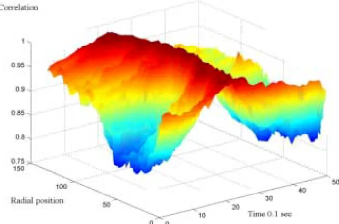
The possibility of extracting quantitative information by image processing of flow struc-tures has been suggested by us a long time ago. The idea arose because we have access to dynamic neutron radiography images of two-phase flow, taken by the Kyoto University Re-search Reactor Institute (KURRI) staff. The images are available as video recordings. Ex-tracting time-dependent intensity data from various pixels, corresponding to various geometrical points in the flow, could make it possible to determine flow velocity profile as well as local radial and axial correlation lengths. The idea is that, by determining the distri-bution of the local correlations lengths and velocity profiles, useful information could be ob-tained for developing an objective flow regime indicator, among others.

Performing such an analysis was hindered so far by the difficulty of extracting time-resolved signals from individual pixels, since earlier this required a so-called frame grabber

with manual control for each frame, which resulted in a very slow and time-demanding procedure. However, digital video recording offers quite different, improved data acquisition possibilities. At the same time, in the frame of an on-going project at the Department, digital video recordings were made of the transport of injected ink in pure water, i.e. one-phase flow. These recordings gave the possibility of testing the principles of the method of correlation analysis of video images. In this Stage a first pilot investigation was made. Time-resolved signals from individual pixels of the recording were extracted, and by using two axially displaced pixels along the same streamline, the transit time of the ink in the water could be determined by correlation analysis. By selecting axially displaced pixels at various radial positions, a velocity profile in the pipe could be determined. The results are quite encouraging and a thorough investigation of the two-phase flow recordings is planned in the continuation.

Forskningsprogram angående härddiagnostik

och härdövervakning med neutronbrusmetoder: Etapp 9

Sammanfattning

Denna rapport redovisar det arbete som utförts inom ramen för ett forskningskontrakt mellan Avdelningen för Reaktorfysik, Chalmers tekniska högskola och Statens Kärnkraftinspektion (SKI), kontrakt Nr. 14.5-020984-02274. Rapporten är baserad på arbetsinsatser av Vasiliy Arzhanov, Anders Nordlund, Dan Olsson och Imre Pázsit, med sistnämnde som projektledare.

Rapporten omfattar etapp 9 i ett långsiktigt forsknings- och utvecklingsprogram angående utveckling av diagnostik och övervakningsmetoder för kärnkraftreaktorer. De långsiktiga målen med programmet har utarbetats i slutrapporterna för etapp 1 och 2 (SKI Rapport 95:14 och 96:50, Ref. [1] och [2]). Uppnådda resultat fram till etapp 8 har redovisats i referenserna [1] - [8]. Ett förslag till fortsättning av programmet i etapp 10 redovisas i slutet av rapporten.

Det utförda forskningsarbetet i etapp 9 består av fyra olika delar och arbetet i varje del sammanfattas nedan.

Utveckling av reaktorkinetik och dynamik i härdar med icke-stationära gränser Studier av rum- och tidsberoende neutronflöden i system med icke-konstanta volymer, dvs sådana som har tidsberoende gränser, har redan inletts vid avdelningen. De motiverades med behovet av att beräkna det neutronbrus som induceras av vibrerande styrstavar och härdhöljevibrationer. En generell formalism har utvecklats inom ramen för linjär brusteori i engruppsapproximationen och homogena system utan reflektor. Inom denna formalism har vi erhållit lösningar på sluten form samt att det ursprungliga problemet med en rörlig gräns kan ersättas med en absorbator med varierande styrka, placerad vid det stationära systemets statiska gräns.

I den här etappen har vi utvecklat teorin och formalismen i två olika riktningar. För det första har vi i den linjära teorin utökat behandlingen till flera energigrupper, fördröjda neutroner och inhomogena härdar. Vi fann att formalismens struktur är oförändrad, med vissa generaliseringar som i den tidigare modellen, med möjlighet till lösningar på sluten form och förenkling av perturbationen med absorbatormodellen. Denna utökning kommer att bli användbar i senare arbeten där vi planerar att undersöka härdhöljevibrationerna i en reaktormodell med reflektor i tvågruppsteori. Den andra utökningen rör behandlingen av stora gränsförflyttningar, till exempel i beskrivningen av den gungande rörelsen hos en fissil lösning, när perturbationsteorin inte går att tillämpa. Vi fann att stora förändringar i systemets form kan leda både till en ökning och minskning av systemets k_eff, beroende på geometrin hos det ursprungliga systemet. Dessa resultat är viktiga för kriticitetssäkerhet i upparbetnings- och anriktningsanläggningar.

Teori och dynamik av källdrivna underkritiska system

De olika reaktorkinetiska approximationerna, t.ex. den punktkinetiska, den adiabatiska och den kvasistatiska, är viktiga i ett antal diagnostiska problem och beträffande parameteruppskattning, inklusive reaktivitetsmätningar. Giltigheten hos de olika approximationerna har undersökts i kritiska och svagt underkritiska härdar. Formalismen hos dessa approximationer, på vilka undersökningarna av deras giltighet är baserad, är inte

direkt applicerbar på källdrivna underkritiska härdar. Mätning av reaktiviteten i en härd under uppstart representerar ett fall hos en källdriven underkritisk härd där giltigheten hos t.ex. den punktkinetiska approximationen på vilken de flesta reaktivitetsmätningar baseras inte har förståtts ordentligt. Sålunda har vi föreslagit en systematisk definition av de kinetiska approximationerna i underkritiska källdrivna härdar, en studie av de relaterade formalismerna och en undersökning av giltigheten hos approximationera. I den här etappen har vi jämfört fördelarna och nackdelarna hos egenfunktionernas utveckling för dynamiken hos kritiska och underkritiska härdar. Det visade sig att både den punktkinetiska och den adiabatiska approximationerna behöver omdefinieras i underkritiska härdar jämfört med kritiska för att få en konsistent beskrivning samt en fysiskaliskt tolkning.

Förberedelser till att konstruera en ny typ av Cf-252 detektor

Ett doktorandprojekt pågår vid vår avdelning angående teorin hos den s.k. Cf-252 metoden för mätning av reaktiviteten i underkritiska härdar. En viktig del i metoden är användningen av en Cf-252 detektor. Källan kombineras med en detektor som detekterar fissionsprodukterna, vilket gör att man kan registrera de neutronemitterande processerna utan att neutronerna absorberas. Signalen från Cf-252 detektorn korreleras därefter med två andra neutrondetektorer som mäter efterföljarna till källneutronerna efter att de initierat fissionskedjan.

De befintliga Cf-252 detektorer som använts av andra har så långt varit av jonkammartyp, där Cf-252 källan fixerats elektrolytiskt på en av jonkammarens plattor. Vi har föreslagit en annan, enklare konstruktion som har sitt ursprung i en liten scintillationsdetektor som tidigare användes som neutrondetektor. Genom att ersätta neutronomvandlaren med Cf-252 kunde en liten Cf-252 detektor konstrueras. Vi fann att det är fullt möjligt att tillverka en fungerande Cf-252 detektor med scintillationsprincipen och att detektorn går att tillverka på Chalmers. Vi kommer därför att fortsätta med att konstruera en sådan detektor och testa den i riktiga mätsituationer.

Dynamiska rumsberoende korrelationsmätningar för enfasflöde med användning av färg och bildbehandling

Möjligheten att få ut kvantitativ information genom bildbehandling av flödesstrukturer har föreslagits av oss länge. Idén dök upp eftersom vi har tillgång till bilder av tvåfasflöde från dynamisk neutronradiografi, tagna av forskare vid Kyoto University Reseach Reactor Institute (KURRI). Bilderna finns tillgängliga som videoinspelningar. Att extrahera tidsberoende intensitetsdata från olika pixlar, motsvarande olika geometriska punkter i flödet, kan göra det möjligt att bestämma såväl flödets hastighetsprofil som lokala radiella och axiella korrelationslängder. Idén är att fördelningen av de lokala korrelationslängderna och hastighetsprofiler ska ge information som kan användas för utvecklandet av en objektiv flödesregimsindikator.

Att genomföra en sådan analys har försvårats tidigare av problem med att extrahera tidsuppslösta signaler från enstaka pixlar eftersom detta tidigare krävt en s.k. “frame grabber” med manuell kontroll för varje bild, vilket ger långsam och tidskrävande databehandling. Digitala videokameror ger helt andra och förbättrade möjligheter att samla in data. Inom ramen för ett pågående projekt vid avdelningen gjordes videoinspelningar av färg som injiceras i rent vatten, dvs enfasflöde. Dessa inspelningar gav möjlighet att testa principerna för metoden med korskorrelationsanalys av videobilder. I den här etappen gjordes en pilotstudie. Tidsupplösta signaler från varje pixel på bilden extraherades och

genom att använda två axiellt separerade pixlar kunde färgens transporttid bestämmas genom korrelationsanalys. Genom att välja axiellt separerade pixlar på olika radiella avstånd kunde en hastighetsprofil i röret bestämmas. Resultaten är uppmuntrande och en grundlig undersökning av bilderna från tvåfasflödesmätningarna planeras i framtiden.

Section 1

Development of reactor kinetics and dynamics for systems with non-stationary boundaries

1.1 Introduction

In our previous work, the need of treating systems with a non-stationary (i.e. moving or oscillating) boundary arose in several problems. The basic question is the calculation of the space- and time-dependent neutron oscillations induced by the oscillating boundary. One classical case is the calculation of the neutron noise induced by vibrating absorbers and fuel rods. Another case is the treatment of the various vibration modes of the core and the core barrel. Finally, the free liquid surface of a molten salt system or a fuel solution in a reprocessing or enrichment plant can also oscillate in time and space, affecting thereby the criticality of the system as well as leading to neutron noise.

The case of the vibrating absorber and the core barrel vibrations has been treated earlier by us. In this Section first a further development of these methods is reported briefly. Namely, the formalism has been elaborated for, and was used so far with, a one energy group treatment. In order for getting a correct description of the core-barrel vibrations when the surrounding reflector is properly taken into account, a two-group treatment is necessary. A generalisation of the previous theory, and the formal solution with the Green’s function technique, was made to a multi-group approach. It was shown that the same closed form formal solution can be obtained in many-group theory as with one-group theory.

The closed form solution mentioned above is possible because these cases, i.e. small vibrations, can be handled by some approximations, such as simplifying a control rod into a Dirac delta function, or replacing the oscillating boundary with a variable strength thin layer of absorber (delta-function in the direction normal to the boundary), placed at the boundary. However, these approximations are based on the application of linear theory, due to the small displacements of the boundary (compared to both the system size and the diffusion length). This is applicable for the case of control rod and core barrel vibrations. The rocking and waving motion of the free surface of a solution of fissile material, on the other hand, does not fulfil the requirement of small shape changes. Hence the treatment of such a problem, and even the calculation of the reactivity as a function of the change of the surface, requires methods that go beyond the limitations of linear theory. In the present chapter such a case is treated. A method is elaborated for the solution of the criticality as a function of the (large) movements of a free surface. It is found that, contrary to intuitive expectations, with the rocking motion of the free surface, an originally critical system can become both super- and subcritical, despite of the increase of the free surface with constant volume (due to which one would expect larger leakage and hence always a decrease in the criticality). This is reported in the second part of the present Section.

1.2 Multi-group approximations for systems with moving boundaries

The recent interest in the noise by vibrating surfaces and interfaces originates from the need of treating the vibrations of a strong absorber [9], [10]. Another case is that of the core barrel vibrations, which have been diagnosed so far through the ex-core neutron noise, which is induced by the varying water thickness between the outer core surface and the pressure vessel [11]. However, the fluctuation of the boundary will also induce in-core

noise in the case of shell-mode vibrations. For the treatment of small variations (vibrations) of the boundary, there are several methods available, which are all equivalent: a time-dependent extrapolation length at the static boundary [10], the assumption of a time-varying absorbing layer at the static boundary, and the recently developed method of coordinate transformations [9]. The equivalence of these methods was first proven for the simpler case of a slab reactor with one fixed and one varying boundary [10], then for the more complicated case of a vibrating absorber rod [9]. In addition, the point kinetic and adiabatic perturbations were also developed and investigated in [10] and [12].

The above investigation, however, all treated a specific, and geometrically simple variation of the boundary. It is of interest to extend the theory to the general case of arbitrary variations of the boundary. In Ref. [12] such a theoretical analysis was given. However, the analysis relied on

• one energy group, one prompt and one average delayed neutron group diffusion approxi-mation;

• homogeneous reactor model.

There is both an academic and a practical interest in extending the formalism of the one group homogeneous model. One question is how the method will work if we drop the limitations. From the practical point of view, treatment of the in-core and in-vessel noise by core barrel vibrations requires the use of two-group theory. To address these questions, the following generalisations of the theory and the associated solutions have been performed: • extension to a multi-group diffusion model with several delayed neutron groups; • treatment of a non-homogeneous reactor model.

A multi-group absorber model has been proposed, which states that, mathematically, the problem of vibrating boundaries is equivalent to placing an infinitely thin absorber of varying strength onto the boundary surface, with a one-to-one mapping of the vibration amplitude normal to but along the boundary to the amplitude of absorber strength fluctuations.

The absorber model turns out to be very useful in extending the formalism of reactor kinetics, including the reactor kinetic approximations such as the point reactor and adiabatic approximations of the neutron noise induced by small but arbitrary fluctuations of the boundary. In addition, the absorber model gives an opportunity to obtain in an elegant way a representation of the neutron noise through the adjoint function of the static problem. This is important for certain practical problems because in energy dependent cases, such as the multi-group approximation, the adjoint function approach has certain advantages over the Green's function method. The work performed in this subject has been published in detail in Annals of Nuclear Energy [13]. For reasons of brevity, the work will not be described here, we refer with the details to Ref. [13].

1.3 Rocking free surface problem

Another practical example of a multiplying system with a time-dependent boundary is the so-called rocking surface problem [15]. For example, when transporting a solution tank of fissile material at an enrichment or reprocessing plant, one needs to know how safe this transport is. Besides the space and time dependent flux variations, even simpler quantities, such as the time dependence of the reactivity, are of vital importance. For instance, it is important to know whether the multiplication factor of the system can increase as compared to the one being at rest? The common physical sense suggests the negative answer because

it relies on the reasoning that, if we increase the outer surface while preserving the volume, the surface leakage of neutrons must increase. However, as it will be shown below, this intuitive expectation does not always hold.

Although one could envisage a variety of shapes for the surface, for simplicity let us assume that it is flat and simply rocks about the midpoint M.

The rocking angle θ = θ(t) can be either a random or deterministic function of time. However, if one introduces time, then we have time-dependent problem which it is best to avoid at this stage. Instead let us assume that P(θ) is a probability distribution that leads to a valueθ. If one can find k_eff(θ) then we may find the statistical moments

(1)

where 0 <θ <θ_m, θ_mbeing the maximum rocking angle.

Ordinary perturbation theory is not applicable here unless the tilt angle is very small. Alternatively, one has to use either direct numerical methods to calculate k_eff(θ) or apply more sophisticated mathematical theory. We are going to demonstrate both approaches. 1.4 Mathematical model

Let us consider the problem in X-Y geometry illustrated by Fig. 1 where the surface (upper side) is allowed to simply rock about a middle point M andθdenotes the tilt angle. We are going to investigate what happens to the effective multiplication factor k_effif we let the angleθ vary from 0 toθ_max = arctan(2H/a).

M

θ

.

Fig. 1. Free surface problem

a

H

∆

b

k_effn 〈 〉 k_effn ( )θ P( ) θθ d 0 θm

∫

=

We assume a one-group diffusion model with space and time independent coefficients. Then k_eff is found as the leading eigenvalue of the following equation

(2)

We set D = 1 cm,Σ_a = 0.1 cm-1, and adjust νΣ_f such that the unperturbed system i.e. the one with θ = 0 becomes critical k_eff = 1. By equating the material and geometrical bucklings for the rectangular system we can express the fission cross section as

(3)

1.5 Numerical simulation

Let the tallness factorτ be defined as

(4)

We first consider a “tall” system with a = 100 cm and H = 400 cm (τ = 4). The criticality condition (2) gives νΣ_f = 0.1010 cm-1. A Matlab code which applies the finite-difference method to find k_eff as function of the tilt angle θ produces an expected result shown in Fig. 2A. The k_eff of the system decreases monotonically with increasing tilt angle.

D∇2φ( )r νΣf k_eff ---–Σ_a    _{ φ( )r} + = 0 φ( )r _Γ = 0      B_m2 (νΣf –Σa) D --- π a ---   2 π H ---   2 + ≡B2_g = ≡ ⇒νΣ_f = B2_gD+Σ_a τ = H a⁄

Fig. 2. k_eff dependence on the angle for tall, flat, and middle systems, Fig.C and Fig.D display the same data on different scales

0 20 40 60 80 0.996 0.997 0.998 0.999 1 K eff ( θ )

Fig.A Tall System

Expected Behaviour τ = 4 0 10 20 30 1 1.001 1.002 1.003 1.004 1.005

Fig.B Flat System

Unexpected Behaviour τ = 1/4 0 10 20 30 40 −5 −4 −3 −2 −1 0x 10 −6 Angle θ [deg] K eff ( θ ) − 1

Fig.C Middle System

τ≈ 0.5 τ = 4 0 20 40 60 0.9999 1 1.0001 1.0002 1.0003 1.0004 1.0005 Angle θ [deg] Fig.D All Systems

τ = 1/4

τ≈ 0.5

By swapping the base and height we keep the fission cross section unchanged, i.e. now we have a = 400 cm, H = 100 cm (τ = 1/4), and again νΣ_f = 0.1010. For this system, however, the k_eff behaviour changes dramatically (Fig. 2.B). The k_eff increases monotonically with increasing tilt angle.

It was found numerically that a “medium-tall” or “medium-flat” system, or just medium system for simplicity, with a = 400 cm, H = 200.0305 cm (τ=0.5001) exhibits a non-monotonic behaviour of k_eff as shown in Fig. 2.C. In this case the change in k_eff is visible only on a very fine scale (change in k_eff is less than 2*10-6). Because of this we plotted k_eff - 1 vs. θ. Fig. 2.D reproduces the same plot as Fig. 2.C to conclude that practically k_eff for the medium system is constant relative to the other systems.

1.6 Analytical estimate for k_eff

To simplify mathematics we slightly rearrange the geometry, as shown in Fig. 3.

The area and boundary of the perturbed system are denoted as S and Γ respectively, whereas refer to a larger rectangle that embraces the tilted one. For future reference we present here some elementary geometric relations

(5)

Mathematically, the problem is to evaluate the minimal eigenpair (k2,ψ) of the equation (6)

x

y

gravity

a

b

c

H

∆

θ

∆

Γ

S

γ

(x)

Γ

'

S

’

Ground

Fig. 3. Perturbed (full line) and static (broken line) systems

S' and Γ' ∆ b 2 ---tanθ = c = H –∆ a = H +∆ y = γ( )x = cot( )θ ⋅x ∇2_ψ k2ψ + = 0 i n S ψ _Γ = 0 on Γ ∂≡ S   

The eigenvalue, k, and the effective multiplication factor k_eff are related to each other as follows.

(7)

One possible solution is to express (k2,ψ) in terms of an other problem, namely,

(8)

for which we know the eigenpairs

(9)

To derive a relationship betweenψandφnwe multiply (6) byφnand (8) byψ, subtract

each other and integrate over the embracing region . Taking into account the boundary conditions we end up with

(10)

Let us define new functions

(11)

Obviously(10), we have

(12)

We representψ as a series

(13)

To find k2 it is sufficient to put the expansion into (10) yielding

(14) k2 νΣ_f k_eff ---–Σ_a D ---= k_eff νΣf k2D+Σ_a ---= ∇2_φ n kn 2_φ n + = 0 i n S' φ_n Γ' 0 = on Γ'≡∂S'      k_n2,φ_n ( ) n≡(n₁,n₂) k_n2 k_n 1 2 k_n 2 2 + πn1 a ---   2 π_n 2 b ---   2 + = = φ_n(x y, ) 2 ab --- πn1x a --- πn2y b ---sin sin =        S' φ_n∂ψ_∂ n ---dl γ

∫

(k_n2–k2) φ_nψdS S

∫

= ∀n Φ_p(x y, ) φp(x y, ) (x y, )∈S 0 (x y, )∉S    ≡ Φ_p N_rpφ_r r

∑

= N_qp φ_p S

∫

φ_qdS ≡ Φ_pφ_qdS' S'

∫

= N_rp φ_r S'

∫

r

∑

= φ_qdS' ψ c_pΦ_p p

∑

= ψ x_pφ_p p

∑

= x_p φ_n∂φ_∂ p n ---dl γ

∫

p

∑

(k_n2–k2) x_p φ_nφ_pdS S

∫

p

∑

=

It is convenient to define the coefficients Anp as

(15)

Then (14) becomes

(16)

Slightly rearranging terms we derive

(17)

By introducing infinite matricesΛ, N, A and a vector

(18)

we arrive, finally, at the basic equation

(19)

which gives k2 as an eigenvalue of the infinite matrix equation (19). Rather strenuous calculations give in the end

(20)

Here

(21)

(22)

The coefficientsα_i and β_i are defined as follows:

(23)

They involve the constants

(24)

The following useful relations hold true

A_np φ_n∂φ_∂ p n ---dl γ

∫

≡ A_npx_p p

∑

(k_n2–k2) N_npx_p p

∑

= ∀n k_n2 N_pnx_p p

∑

A_npx_p p

∑

– k2 N_npx_p p

∑

= ∀n x Λ k₁2 0 k₂2 0 … ; ≡ N ≡ N_np ; A≡ A_np ; x x₁ x₂ … ≡ ΛN –A ( )x = k2N x A_mn 1 a2 --- C₁Sin2α1π 2 --- C₂Sin2α2π 2 ---– ; m ≡ = (m₁,m₂); n = (n₁,n₂) C₁ (σn₂+n₁) 1 α₁ --- _β1 3 ---+     _σn 2–n1 ( ) 1 α₃ --- _β1 1 ---+     + = C₂ (σn₂–n₁) 1 α₂ --- _β1 4 ---+     _σn 2+n1 ( ) 1 α₄ --- _β1 2 ---+     + = α₁≡(m₂–n₂) η– (m₁–n₁) β₁≡(m₂–n₂) η+ (m₁–n₁) α₂≡(m₂–n₂) η– (m₁+n₁) β₂≡(m₂–n₂) η+ (m₁+n₁) α₃≡(m₂+n₂) η– (m₁–n₁) β₃≡(m₂+n₂) η+ (m₁–n₁) α₄≡(m₂+n₂) η– (m₁+n₁) β₄≡(m₂+n₂) η+ (m₁+n₁) σ tan aθ b

--- tanθ(τ+0.5tanθ) η btanθ a --- tanθ τ+0.5tanθ --- τ H b ---≡ ; = ≡ ; = ≡

(25)

The coefficients N_mn were found to be

(26)

The above formulas constitute a formal solution to the problem. In practice, the size of the problem and the rank of the associated matrices need to be chosen as finite, by cutting the expansions (13)-(17) after a finite number of terms. The critical buckling is then obtained as the leading eigenvalue of eqn (19), which is then of finite order. No numerical evaluations of the problem have been done so far.

1.7 Conclusions

The examples presented in the paper show that enlargement of the outer surface while keeping the volume constant does not necessarily lead to reduction in the criticality of a fissile system through increase of neutron leakage. From the theoretical point of view the explanation lies in the fact that it is not the size of the outer surface alone that determines the leakage, rather the integral

(27)

Now the current (flux gradient) also changes on the boundary when the boundary is moved, hence the integral in (27) does not behave in a simple way. From the practical point of view it is important to account for this non-trivial effect of the free surface for example when dealing with solutions of multiplying material both in reprocessing plants and in molten salt type future accelerator driven systems.

1 α₁ --- 1 β₃ ---+ 2m2 m₂2–[n₂+η(m₁–n₁)]2 ---= 1 α₃ --- 1 β₁ ---+ 2m2 m₂2–[n₂–η(m₁–n₁)]2 ---= 1 α₂ --- _β1 4 ---+ 2m2 m₂2–[n₂+η(m₁+n₁)]2 ---= 1 α₄ --- 1 β₂ ---+ 2m2 m₂2–[n₂–η(m₁+n₁)]2 ---= N_mn N_mn Amn– Anm k_m2 –k_n2 --- m≠n = π 1 η 2 ---–     n2 2 2ηπ2n₁2(n2₂–η2n₁2) ---Sin2(ηn₁π) m + = n = (n₁,n₂)          = ∂φ ∂n ---dS S≡

∫

∂V

Section 2

Theory and dynamics of source-driven subcritical systems

2.1 Introduction

There are several classical methods that have long been used for the description of the kinetics and the dynamics of critical or non-critical but source-free systems. Two such classical methods are the eigenfunction expansion and the so-called kinetic approximations (point kinetic, adiabatic, quasistatic), the latter being based on the flux factorisation (Henry factorisation) ([17], [18]) into an amplitude and a shape function. There exist of course numerous other, purely numerical schemes for the solution of the space-time-energy dependent neutronic equations, but the power of the classical methods is that they lend physical insight into the behaviour of the system. This is because certain terms of the solution dominate asymptotically as a function of some parameter, and moreover it is very easy to develop an intuitive feeling for such terms, such as the effect of a reactivity change, or the adiabatic distortion of the flux shape etc. This is especially true for the case of neutron noise, induced by stationary and small fluctuations of the cross sections, which will be one of the cases that we investigate.

The dynamic behaviour of source-driven subcritical systems has recently become interesting for several reasons. One reason is due to the increasing popularity of the concept of accelerator-driven subcritical systems (ADS). Another is that measurement of reactivity in a sub-critical system during startup with an extraneous source has received enhanced interest in connection with the incident at the French PWR Dampierre-4. The Department of Reactor Physics at Chalmers has started a PhD project for investigating the effectiveness of the Cf-252 source based and similar stochastic reactivity measurement methods. In all cases the system under investigation is a source-driven subcritical cores. It is obvious that these systems have physical properties that are different from those of critical or source-free systems. Therefore, not surprisingly, the mathematical tools to be used for their description need to be modified. Moreover their properties, including their applicability, will also be different from those in source-free systems.

The purpose of this Section is to investigate two classical methods for the description of source-driven systems. One is the eigenfunction expansion, and the other is the kinetic approximations, based on the flux factorisation technique. The physical situations that we investigate by both of these methods will also consist of two simple basic cases. One is the attainment of the asymptotic behaviour of the flux in a steady system from an arbitrary initial flux shape; the other is the space and frequency dependent response of a system for small, stationary fluctuations of the cross sections. The emphasis is on the physical meaning of the solutions, and on the differences between the source-free and the source-driven cases. The source-driven subcritical case will be described by an extraneous source within the core. This is an approximation used to simplify the situation. Other descriptions are also possible, such as separating the source from the core and imposing the effect of the source through coupling at the interface [19]. The emphasis is however in both descriptions on the fact that the system is source- (or boundary condition)-driven, with relatively loose coupling between different spatial points of the system. This will determine much of the physical properties.

The results described in this Section were presented at the ANS meeting “American Nuclear Society Topical Meeting in Mathematics & Computations”, Gatlinburg, TN, 2003 (Ref. [20]).

2.2 The eigenfunction expansion

Throughout in this Section, we shall use one-group diffusion theory, and one group of delayed neutrons, to keep the reasoning simple. Extension to more complicated cases is straightforward. In what follows, we shall treat two simple cases of time- (or frequency)-dependent solutions: the approaching of the asymptotic state of the flux in a stationary system, and the neutron noise induced in the system by small fluctuations of the cross sections.

Asymptotic solutions in a steady system Source-free system

In a source-free, critical or non-critical system, the diffusion equation can be written symbolically as

(28) The diffusion operator is assumed to have a complete orthogonal set of eigenfunctions

. Using the concept of the -eigenfunctions [18], these are defined as

(29) Actually in this notation it is implicitly assumed that the delayed neutrons are neglected. It is easy to extend the formalism to include even these, but for the simple argument we want to make here it is not necessary. It is straightforward to show that with the use of the expansion (29), the solution of (28), for any given initial condition

(30) is given as

(31) The coefficients can be determined from the initial condition (30) as

(32)

As is known, the eigenvalue with the largest real part, , is real, and the corresponding

eigenfunction, the fundamental mode , is non-negative. The asymptotic behaviour is

therefore

(33)

and the other eigenvalues describe, through (31), how fast the system reverts to the

1 v ---∂φ(r t, ) ∂t --- = L⋅φ(r t, ) L φ_n( )r α Lφ_n( )r = α_nφ_n( )r φ(r t=0, ) φ≡ ( )r φ(r t, ) a_n( )φt _n( )r n=0 ∞

∑

a_neαntφ n( )r n=0 ∞

∑

= = a_n a_n φ( )φr _n( )r dr

∫

φ_n2 r ( )dr

∫

---= α α₀ φ₀( )r φ(r t, ) a₀eα0tφ 0( )r → α_n

asymptotic state. It is also seen that the asymptotic behaviour is point kinetic, i.e. the space-time dependence of the flux is factorised into a space-time-dependent amplitude factor, and a shape function which is identical with the fundamental mode, i.e. the fundamental eigenfunction of

the diffusion operator. As is also well known, for a critical system , i.e. the

asymptotic solution is time-independent. For the case , no time-independent solutions exist.

Source-driven system

For the source-driven subcritical system, the equation corresponding to (28) is written as

(34) Here we only treat the case of a time-independent source, in which case (34) always has a

time-independent static solution , obeying

(35) To describe the relaxation of the system from an arbitrary initial condition to the static solution, one can still use the eigenfunction expansion method, although in a slightly modified way. The eigenfunctions to be used are still those of the operator . However, the

static (asymptotic) solution is no longer an eigenfunction of . An expansion of the

flux in the form (31) is therefore not practical in this case, since the asymptotic form would

consist of the expansion of into the eigenfunctions and hence the transition to

the asymptotic form would not be easily visible. It is therefore more practical to seek the time-dependent solution in the form

(36) From (34)-(36) it is seen that satisfies the homogeneous (source-free) equation (28), hence its solution is worth to be given in the form of an eigenfunction expansion. This will yield the same result as (31), i.e.

(37) with the only difference that the coefficients are now given by

(38)

Hence the full time-dependent solution is given as

(39)

Since the system is subcritical, , and the whole sum in the r.h.s. of (39)

vanishes with increasing time. Eqn (39) shows the transition to the asymptotic state, and it is seen that this transition is not point kinetic. The speed of the initial flux shape to revert to the

α₀ = 0 α₀≠0 1 v ---∂φ(_∂r t, ) t --- = L⋅φ(r t, )+S( )r φ_s( )r Lφ_s( )r +S( )r = 0 L φ_s( )r L φ_s( )r φ_n( )r φ(r t, ) = φ_s( ) ϕr + (r t, ) ϕ(r t, ) ϕ(r t, ) a_neαntφ n( )r n=0 ∞

∑

= a_n a_n φ( ) φr – _s( )r [ ] ( )φ_n( )r dr

∫

φ_n2 r ( )dr

∫

---= φ(r t, ) φ_s( )r a_neαntφn( )r n=0 ∞

∑

+ = ℜe( )α_n <0, ∀n

asymptotic depends on the eigenvalues . In general, the deeper the system subcriticality, the faster the asymptotic state is reached. There is no similar statement for the source-free system, because there the speed of approaching the asymptotic state depends on the ratio between the real parts of the fundamental and higher order eigenvalues.

Neutron noise induced by cross section fluctuations Source-free (critical) system

For this case now we select a concrete representation of the diffusion operator,

corresponding to a bare homogeneous system. Hence, for a source-free system, the time-dependent equations read as

, (40)

(41) We will assume that without perturbations the system is critical, described by

(42) and

(43) with

(44) and with the usual diffusion theory boundary condition

. (45)

We will assume that the dependence of the flux is brought about by the space- and time-dependence of the absorption cross sections:

(46) Since the small cross section fluctuations will induce small flux fluctuations and we shall use linearised equations, we write

(47) (48) Putting (46)-(48) into (40)-(41), subtracting the static equations, neglecting the second order

term and eliminating the fluctuations of the delayed neutrons by a temporal

Fourier-transform, one obtains in the frequency domain the following equation for the neutron noise: (49) α_n 1 v ---∂φ(r t, ) t ∂ --- = D∇2φ+[(1–β)νΣ_f –Σ_a]φ(r t, ) λ+ C(r t, ) C(r t, ) ∂ t ∂ --- = βνΣ_fφ(r t, ) λ– C(r t, ) ∇2_φ 0( )r B0 2_φ 0( )r + = 0 βνΣ_fφ₀( )r = λC₀( )r B₀2 νΣf –Σa D ---= φ( )r_B = 0 Σ_a→Σ_a+δΣ_a(r t, ) φ(r t, ) = φ₀( )r +δφ(r t, ) C(r t, ) = C₀( )r +δC(r t, ) δΣ_a(r t, ) φδ (r t, ) ∇2 _φ r,ω ( ) δ +B2( ) φω δ (r,ω) S r( ,ω) φ0( )r D ---⋅δΣ_a(r,ω) ≡ =

with representing the “noise source” whereas is termed as the perturbation. Further,

(50)

with

(51)

being the zero-reactor transfer function of critical cores.

We shall now seek a solution of (49) with the eigenfunction expansion method as

(52) where the eigenfunctions are now solutions to the equation

(53) with the same boundary conditions as (45). Obviously, criticality requires that in (53) is the same as in (44). Substitution of (52) into (49) yields, using the orthogonality of the

eigenfunctions, an expression for the in the form

(54)

In writing out (52) with (54) it is practical to separate the first term, i.e. that for from the rest:

(55)

where the reactivity of the perturbation, , is given by

(56)

From (55) it is seen that the first term becomes dominant in two distinct cases, so that the last term on the r.h.s. expressed by the sum can be neglected or is vanishing. Whenever this happens, the system behaviour becomes point kinetic, since, again, the time (frequency) and space dependence is factorised, and the space dependence is equal to that of the fundamental mode. The first case of point kinetic behaviour is that of the low frequencies,

S r( ,ω) δΣ_a(r,ω) B2( )ω B₀2 νΣf DG₀( )ω ---– = G₀( )ω 1 iω Λ β iω λ+ ---+     ---= δφ(r,ω) a_n( )φω _n( )r n=0 ∞

∑

= ∇2_φ n( )r Bn 2_φ 0( )r + = 0 B₀2 a_n( )ω a_n( )ω δΣ_a(r,ω)φ₀( )φr _n( )r dr

∫

D –B_n2 B₀2 νΣf D G⋅ ₀( )ω ---– +

∫

φ_n2( )r dr ---= n = 0 δφ(r,ω) δρ ω( )⋅G₀( ) φω ⋅ ₀( )r δΣ_a(r,ω)φ₀( )φr _n( )r dr

∫

– D B_n2–B₀2 νΣf D G⋅ ₀( )ω ---+

∫

φ_n2( )r dr ---⋅φ_n( )r n=1 ∞

∑

+ = δρ ω( ) δρ ω( ) 1 νΣ_f ---δΣ_a(r,ω)φ₀2( )r dr

∫

φ_n2 r ( )dr

∫

---– =

and this observation was made already by Weinberg and Schweinler [21]. As (51) shows, diverges for , whereas all terms in the sum on the r.h.s. of (55) remain finite in this limit. The only exception from this behaviour arises for perturbations whose reactivity effect is exactly zero, i. e. when is orthogonal to . In that case point kinetic behaviour will never occur. The other possibility for point kinetic behaviour is when the perturbation is space-independent, i.e. when

. (57)

or, in other words, when the noise source is proportional to the static flux,

. (58)

In that case, the whole sum in (55) is zero, i.e. for all values. Physically this means that the noise source, due to the perturbation (57), does not excite any of the higher order spatial modes, only the fundamental one, and hence point kinetic behaviour will prevail for any frequency.

Source-driven (subcritical) system

In order to distinguish that the system is now not critical we shall use slightly different notations. Eqn (40) is now replaced by

(59) and the static equation by

(60) The subscript “s” indicates the source-driven subcritical case, in order to distinguish from the geometrical buckling (fundamental eigenvalue) and the fundamental mode. In (60), stands for the static (non-critical) material buckling

(61)

The buckling corresponding to the fundamental mode is related to the above as

(62) Here is the static subcriticality of the source-driven system, not to be mixed up with the reactivity effect of the perturbation, .

To arrive to the noise equations, one again assumes that the time (frequency) dependence is induced by the fluctuations of the absorption cross sections, eqn (46). However the neutron noise needs to be defined as the deviation from the static subcritical flux, i.e. in contrast to (47) one writes

(63) Repeating now the same steps as the one leading to (49) will lead to a formally similar equation in the form

G₀( )ω ω→0 δΣ_a(r,ω) φ₀2( )r δΣ_a(r,ω) = δΣ_a( )ω S r( ,ω) φ0( )r D ---⋅δΣ_a( )ω = a_n = 0 n 1 v ---∂φ(r t, ) t ∂ --- = D∇2φ+[(1–β)νΣ_f –Σ_a(r t, )]φ(r t, ) λ+ C(r t, )+S( )r ∇2_φ s( )r Bs 2_φ s( )r + = S( )r B_s2 B2_s νΣf –Σa D ---= φ₀( )r B₀2 νΣf ⁄k –Σa D --- B_s2 ρsνΣf D ---– = = ρ_s δρ φ(r t, ) = φ_s( )r +δφ(r t, )

(64) with

(65) One can now again seek the solution of (64) in the same form as in (52). After the same manipulations as before one arrives at the solution

(66)

Here

(67)

is the zero reactor transfer function of subcritical cores [22], and the reactivity perturbation is given as

(68)

The properties of the solution (66) are different from those of (55), therefore (66) is less suitable for the analysis of the asymptotic properties of the system. These differences are related to the differences in the physics of the two cases (critical and source-driven systems). First of all, in a source-driven system the point kinetic approximation means a space-time factorisation in which the space dependence is equal to that of the static flux . It is not possible to easily discern any asymptotics in (66) which would lead to such a behaviour. In particular, and in contrast to (55), the first term on the r.h.s. does not represent the point kinetic term. Consistently, this term does not become dominant either in any of the two cases which led to point kinetic behaviour in the critical system. What regards the case of low frequencies, as (67) shows, remains finite even for , hence low frequencies do not induce the dominance of the first term. Likewise, since the static flux is not orthogonal to any of the eigenmodes , a spatially constant perturbation will not lead to the vanishing of the sum in (66) since the static flux is not orthogonal to any of the eigenmodes .

Based on the postulation of point kinetic behaviour in the form of

, (69)

one can try to use an expansion similar to (36) and (37) in the hope of extracting the conditions of point kinetic behaviour. That is, one writes

∇2 _φ r,ω ( ) δ +B_s2( ) φω δ (r,ω) S r( ,ω) φs( )r D ---⋅δΣ_a(r,ω) ≡ = B_s2( )ω B_s2 νΣf DG₀( )ω ---– = δφ(r,ω) δρ ω( )⋅G_s( ) φω ⋅ ₀( )r δΣ_a(r,ω)φ_s( )φr _n( )r dr

∫

– D B_n2–B₀2 νΣf D G⋅ _s( )ω ---+

∫

φ_n2( )r dr ---⋅φ_n( )r n=1 ∞

∑

+ = G_s( )ω 1 iω Λ β iω λ+ ---+    _{ ρ} s – ---= δρ ω( ) _νΣ1 f ---δΣ_a(r,ω)φ_s( )φr 0( )r dr

∫

φ₀2 r ( )dr

∫

---– = φ_s( )r G_s( )ω ω = 0 φ_s( )r φ_n φ_s( )r φ_n( )r A( )φω _s( )r

(70) This trick is, however, not as effective in the present case as in Section 2.1 treating the asymptotic behaviour in a steady system. Executing the same steps as before will lead to

(71)

For this can be simplified to

(72) From (72) it is seen that the frequency tending to zero is not sufficient alone to grant the validity of the point kinetic approximation. It is also necessary that the perturbation

has a special form. It can be shown that if the noise source can be factorised into a frequency dependent factor and a spatial shape equal to that of the static source, i.e.

, (73)

then

(74) and

(75) is a solution of (72). That is, for vanishing frequencies, and a noise source that factorises as the static source, one will have

(76) This solution has already been derived in [23] with much less effort with the use of the Green’s function technique. However, this solution is rather formal and useless, since, strictly speaking, it is only valid for . It is at any rate not suitable to investigate the domain of validity of the point kinetic approximation with increasing frequencies, only for the demonstration of two facts. One is that low frequency alone is not sufficient to impose point kinetic behaviour on a source-driven system, which is a direct consequence of the physics. The second is the fact that the expansion of the solution of a source-driven system into spatial eigenfunctions of the diffusion or transport operator is rather ineffective in treating neutron noise problems, even in cases of low frequency or a special spatial shape of the perturbation. For the treatment of the reactor noise in source-driven systems the flux factorisation technique and the kinetic approximations are more useful.

2.3 Flux factorisation and the kinetic approximations

The possibility of using the Henry factorisation technique [17] for the definition and analysis of the kinetic approximations in source-driven systems was already investigated in [23]. Apparently only the case of fluctuations of the extraneous source were investigated there, but formally, the noise source of the linearised equations, represented by the fluctuations of the absorption cross sections, play a formally identical role. Hence here we only summarize the

δφ(r,ω) A( )φω _s( )r a_n( )φω _n( )r n=0 ∞

∑

+ = A( )ω νΣf D G⋅ ₀( )ω ---φ_s( )r +S( )r – a_n( )ω [B_s2( )ω –B_n2]φ_n( )r n=0 ∞

∑

+ = S r( ,ω) ω→0 A( )ω S( )r – a_n( )ω [B_s2( )ω –B_n2]φ_n( )r n=0 ∞

∑

+ = S r( ,ω) S r( ,ω) S r( ,ω) = f( )ω S( )r A( )ω = –f( )ω a_n( )ω = 0; ∀n δφ(r,ω) = –f( )ω φ_s( )r ω = 0

main points of the analysis given in [23], by formulating it such that the perturbation can be either fluctuations of the extraneous source, or the cross section fluctuations. The system we investigate will be the same as in Section 2.2 above.

The reactor kinetic approximations are all based on a factorisation of the space-time dependent flux into an amplitude factor and a shape function as follows ([17], [18]). One writes

(77)

where is the amplitude function and the shape function. The idea is that any

change in reactor power should be represented by the amplitude factor, whereas deviations

from the stationary flux shape be represented by the shape function . To this order,

and also to make the factorisation (77) unambiguous, one requires the normalisation condition

(78) where is the fundamental mode, i.e. the solution of the eigenvalue equation

(79) Actually, the choice of the weight function in the normalisation condition (78) is not crucial. Other weight functions are also possible.

We shall also assume that at , i.e. before the perturbation started, one had a stationary system with

(80) from which one has

(81) and

(82) Equations (80) and (82) amount to the fact how the point kinetic approximation is defined, and it is consistent with the earlier definition in Section 2. Namely, deviations of the flux shape from that of the static (subcritical) flux will count as deviation from the point kinetics, whereas all changes of power that do not alter the shape of the static flux will count as point kinetic.

The usual way of developing the reactor physics approximations from (80) and (82) is to derive coupled equations for and . Here we shall only consider the linear case of small perturbations. Then, similarly to the previous case, all time-dependent quantities will be split up to static (expected) values and fluctuations as

(83) (84) φ(r t, ) = P t( )ψ(r t, ) P t( ) ψ(r t, ) ψ(r t, ) t ∂∂ ψ

∫

(r t, )φ0( )r dr = 0 φ₀( )r D∇2φ₀( )r νΣf k_eff ---–Σ_a    _{ φ} 0( )r + = 0 t = –∞ φ(r t =, –∞) = φ_s( )r P t =( –∞)≡P₀ =1 ψ(r t, )φ₀( )r dr

∫

=

∫

φ_s( )φr ₀( )r dr P t( ) ψ(r t, ) φ(r t, ) = φ_s( )r +δφ(r t, ) P t( ) = 1+δP t( )

(85) The perturbation is represented by the fluctuations of the absorption cross section as before, (86) Using (85) in (77) and neglecting the second order terms yields the following expressions in the time and frequency domain:

(87) To obtain equations for the fluctuations of the amplitude, , and the shape function, , one has to substitute the flux factorisation (77) into the time-dependent equations, multiply by the fundamental mode and integrate over the volume of the reactor. One also multiplies equation (79) by , integrates, and subtracts the two equations. This manipulation will lead to the point kinetic equations for in the form

(88)

Here, the following functions have been introduced:

(89)

and

(90)

and is the same as in (64).

The point kinetic equations can be solved by direct temporal Fourier transform of Eqn. (88). Eliminating the delayed neutron precursors leads to the frequency domain solution

(91) where is the zero-reactor transfer function of the subcritical system, given by (67).

The equation for the shape function is more involved, and we shall here only treat two simple cases, i.e. the determination of in the point kinetic and adiabatic approximations. The point kinetic approximation actually means to assume

(92) for all time instants. Thus the space-time dependent flux is given as

(93) ψ(r t, ) = φ_s( ) δψr + (r t, ) Σ_a(r t, ) = Σ_a+δΣ_a(r t, ) φ(r t, ) δ = φ_s( ) δr ⋅ P t( ) δψ+ (r t, ) φ(r,ω) δ = φ_s( ) δr ⋅ P( ) δψω + (r,ω) δP( )ω δψ(r,ω) φ₀( )r ψ(r t, ) P t( ) dδP t( ) dt --- = ρ β---_Λ– δP t( ) λδ+ C t( ) δρ+ ( )t dδC t( ) dt --- = _Λ----βδP t( ) λδ– C t( )      δC t( ) δC(r t, )φ₀( )r dr

∫

1 v ---

∫

φ₀2( )r dr ---≡ δρ( )t S(r t, )φ₀( )r dr

∫

νΣ_f

∫

φ_s( )φr ₀+( )r dr ---– ≡ S(r t, ) P( )ω = G_ρ( )δρ ωω ( ) G_ρ( )ω ψ(r t, ) ψ(r t, ) = φ_s( )r φ(r,ω) δ = φ_s( ) δr ⋅ P( )ω = G_ρ( )δρ ωω ( )φ_s( )r

According to this definition the reactor behaves in a point-kinetic manner as long as the flux shape does not deviate from that of the static flux of the subcritical, source-driven reactor.

The solution in the point kinetic approximation given by (93) is defined for all frequencies. Hence the validity of this approximation can be quantitatively checked against the solution of the full space-frequency dependent equation (64). Such a comparison has been performed for a few specific cases of perturbations in [23]. In accordance with what has been stated in the foregoing, the point kinetic approximation performs well for noise sources having the same shape as the static source, but it breaks down even for low frequencies for other perturbations.

The definition of the adiabatic approximation for source-driven systems is different from what one would intuitively suggest. Since the system is now subcritical, the static equation (60) has always a solution with a time-dependent source at any time instant such that is only a parameter and not a variable. It is tempting to define the adiabatic approximation as determining from such a simple calculation.

However, as is described in [23], such a solution is very poor because in treating a fully static equation, one neglects the contribution from the delayed neutrons completely. At low frequencies this solution would be exact, but with increasing frequencies ( ) the decrease of the amplitude due to the disappearing of the delayed neutrons from the dynamic response would not be accounted for. Thus it is much more efficient to still use the factorisation (77), determine the amplitude factor from the point kinetic equations, and determine the shape function from a static equation by using the normalisation (78). This normalisation is not as trivial as in the case of critical systems, where the shape function has to be determined from an eigenvalue equation and needs to be normalised anyway. By the above described strategy the delayed neutrons (or their absence) are accounted for, even if only with a simple space dependence.

Thus, for the definition of the adiabatic approximation, we re-write the time-dependent equation as

(94) Introducing the factorisation (77) into (94) and neglecting all time derivatives leads to the equation

(95) Actually, eqn (95) can be further simplified. According to (78) or (82), the shape function needs to be properly normalised. If we had not neglected time derivatives when going over from (94) to (95), this would have been granted. However, due to the neglections of the time derivatives, the solution of (95) will not, in general, be properly normalized. Since the solution of (95) depends linearly on the last term (which is the inhomogeneous term in the equation), we can replace the factor with unity, since the normalisation will overrule the effect of it anyway. Thus the adiabatic equation for the shape function will be

(96)

with the further condition that must fulfil the normalisation condition (82). How

the normalisation is achieved is described in [23]. Having found , the fluctuation

φ(r t, ) S(r t, ) t t φ(r t, ) ω λ> P t( ) ψ(r t, ) 1 v ---∂φ(r t, ) t ∂ --- D∇2φ(r t, ) [νΣ_f –Σ_a(r t, )]φ(r t, ) ∂C(r t, ) t ∂ ---– S( )r + + = D ψ_ad(r t, ) [νΣ_f –Σ_a(r t, )]ψ_ad(r t, ) S( )r P t( ) ---+ + ∇2 _{= 0} 1 P t⁄ ( ) D∇2ψ_ad(r t, )+[νΣ_f –Σ_a(r t, )]ψ_ad(r t, )+S( )r = 0 ψ_ad(r t, ) ψ_ad(r t, )