Evaluation of a
sustainable spare part
distribution at Tetra Pak
Sea instead of air transportation and its effects
on supply chain inventories
III
1. Acknowledgements
This master thesis has been an interesting and long journey and the fact that the time schedule has been revised at several occasions has actually contributed to a, hopefully, mature and well thought through conclusion. I want to especially thank Peter Berling for his patience and good discussions, the academic view point and approach is definitively one of the lessons learned through this report.
I would also like to thank Jörgen Siversson and Malin Gyllander for their time and equally strong patience with this report, deadlines is a lesson I obviously still looking forward to learn. Malin and Jörgen´s network inside and outside Tetra Pak has made the data collection phase of this report a smooth transaction and enabled the much appreciated visit in Gothenburg harbour. While on the subject I would like to bring a warm thanks to the people at Geodis Wilson for their helpful attitude and time spent guiding me around the world of transports.
Furthermore I would like to thank all the helpful people within Tetra Pak, in the market companies, Transport and Travel, operations and all other departments that have contributed in one or another way to this report.
IV
V
2. Abstract
2.1 Title
Evaluation of a sustainable spare part distribution at Tetra Pak
Sea instead of air transportation and its effects on supply chain inventories
2.2 Author
Niklas Larsson
2.3 Supervisors
Peter Berling, Department of Industrial Management and Logistics, Lunds Tekniska Högskola Jörgen Siversson, Logistics Expert, Tetra Pak Technical Service AB
Malin Gyllander, Transportation Manager, Tetra Pak Technical Service AB
2.4 Keywords
Supply Chain Efficiency, Transportation mode, Environmental cost
2.5 Purpose
The purpose of the report is to look into the effect of changing from air shipments to sea shipments at Tetra Pak Technical Service AB and the economical and environmental impact of such a change on the supply chain.
2.6 Methodology
The report is carried out by collecting the data regarding the different transportation modes in interviews with responsible persons within Tetra Pak and the transporter Geodis Wilson. The data is then simulated for general materials with suitable parameters and a general graph is generated from the simulations. The graphs are applied to the real life materials and a validation of the model is to be done.
2.7 Conclusion
This report shows that a maritime set up for stock refill between local and central warehouses in the affected routes are generally very interesting for heavy weight materials with high demands. There are several interesting materials even within TSAB (Tetra Pak Technical Service AB) but the spare parts business is not the most suitable area for sea transportation due to the low volumes and erratic
VI
materials. Despite this there are still enough incitements even within these materials to introduce a process to handle the few obviously interesting materials.
Regarding the environmental impact (measured as the emission of carbon dioxide) it´s clear that sea transportation is a more sustainable alternative. But as long as the company policy is unclear regarding the value of reducing the impact or no targets are set to reduce the total impact it´s not feasible to include it as a cost in a separate decision as the one discussed in this report.
VII
Contents
1. Acknowledgements ... III 2. Abstract ... V 2.1 Title ... V 2.2 Author ... V 2.3 Supervisors ... V 2.4 Keywords ... V 2.5 Purpose ... V 2.6 Methodology ... V 2.7 Conclusion ... V 3. Introduction ... 1 3.1 Tetra Pak ... 1 3.2 Technical Service ... 2 3.3 Environmental policy ... 3 3.4 Problem background ... 4 3.5 Problem definition ... 4 3.6 Purpose ... 4 3.7 Objective ... 5 3.8 Target group ... 5 3.9 Delimitations ... 5 4. Methodology ... 7 4.1 Scientific approach ... 7 4.2 Data gathering... 7 4.2.1 Literature Study ... 7 4.2.2 Presentation ... 8 4.2.3 Interviews ... 8VIII 4.2.4 Surveys ... 9 4.2.5 Observations ... 9 4.2.6 Experiments ... 9 4.2.7 In this report ... 10 4.3 Methods of analysis ... 10 4.3.1 Credibility ... 10
4.3.2 Approach depending on knowledge ... 11
5. Tetra Pak Technical Service – Set up ... 13
5.1 Supply chain ... 13
5.1.1 Transportation cost ... 15
5.1.2 Storage cost ... 16
5.1.3 Cost of capital... 17
5.1.4 Environmental cost ... 17
6. Theory - Inventory control systems ... 19
6.1 General ... 19
6.2 Single Echelon System ... 19
6.2.1 Ordering systems ... 19
6.2.2 Ordering quantity ... 20
6.2.3 Service level (Availability) ... 22
7. Empirical data ... 25
7.1 Data collection ... 25
7.2 Transportation cost ... 26
7.3 The local sites ... 27
7.3.1 China ... 27
7.3.2 Brazil ... 27
IX
7.3.4 United States ... 28
7.3.5 United Arab Emirates ... 29
7.4 Sea transportation ... 29
7.4.1 To departing port ... 29
7.4.2 Port to port ... 30
7.4.3 From arriving port ... 30
7.5 Air transportation ... 31
7.5.1 To departing port ... 31
7.5.2 Port to port ... 31
7.5.3 From arriving port ... 32
7.6 Storage cost ... 32
7.7 Cost of capital ... 32
7.8 Environmental cost ... 32
8. Analysis ... 35
8.1 The design of the experiment ... 35
8.2 Results of the experiment ... 37
8.2.1 Gain – Service level target (X/X/X = Price/Weight/Standard deviation)... 38
8.2.2 Gain – Price (X/X/X = Price/Weight/Standard deviation) ... 39
8.2.3 Gain – Weight (X/X/X = Price/Weight/Standard deviation) ... 41
8.2.4 Gain – Volume (X/X/X = Price/Weight/Standard deviation) ... 42
8.2.5 Gain – Demand (X/X/X = Price/Weight/Standard deviation) ... 43
8.2.6 Gain – Demand/Std deviation ratio (X/X/X = Price/Weight/Standard deviation) ... 44
8.2.7 Gain – Environmental cost (X/X/X = Price/Weight/Standard deviation) ... 45
8.2.8 Gain – Transportation cost difference (X/X/X = Price/Weight/Standard deviation) ... 46
X
8.2.10 Gain – Transportation cost difference, demand included (X/X/X/X = Price/Weight/Standard
deviation/Demand) ... 48
8.2.11 Gain - Transportation time difference, demand included (X/X/X/X = Price/Weight/Standard deviation/Demand) ... 49
8.2.12 Summary of the graphs ... 49
8.3 Validation of the total gain formula ... 54
8.3.1 Values inside the ranges ... 54
8.3.2 Values outside the ranges ... 55
9. Results ... 59
9.1 High profit materials ... 64
10. Conclusions ... 67
11. Further investigations ... 71
11.1 Transportation contract ... 71
11.2 Door-2-door service ... 71
11.3 Service level targets/definition ... 71
11.4 Buffer stock calculations ... 71
11.5 Global supplier contracts ... 72
Appendix A – Calculations:... 73
1
3. Introduction
3.1 Tetra Pak
The story of Tetra Pak begun with the company of Åkerlund & Rausing where primarily Ruben Rausing and Erik Wallenberg set out to create a substitute for the milk bottle in glass. Their effort led to the creation of Tetra Pak AB in 1951 and the classical tetrahedron shaped carton package. In 1991 the company of Alfa Laval was obtained, thereby the food section were incorporated in the business and now a complete solution from raw material to finished consumer product became available.1 Today the company has a wide range of packaging alternatives and
processing solutions employing almost 22 000 people worldwide. Their cartons can be found in more than 170 countries and they have a total of 40 Market Companies all over the world. With new emerging markets there has been an exploding sales volume the last decades from 20 billion sold packages 1980 to 158 billion packages sold in 20102.
Creating the fundament on which the company stands is the core values: - Customer Focus & Long-term View
- Quality and Innovation - Freedom & Responsibility - Partnership & Fun
1
Tetra Pak – internal material 2
2
3.2 Technical Service
Supporting this global business is the infrastructure of spare parts distribution which keeps the 9 000 packaging machines, 63 000 processing units and 17 000 distribution equipments around the world running. The sales are executed through a global supply chain with two central warehouses as its backbone, located in Lund and Shanghai. These two locations provide both the local European and Asian end customers and the several local warehouses situated around the world. To cover the full variety of parts around 1000 different external suppliers are used and approximately 60 000 articles are sold somewhat frequently.3 The complexity is not dampened by the internal variety and inherited cultural differences between the processing and packaging divisions which are still handled separately to a wide extent. Adding to this is a pallet of side businesses which is mainly ice cream lines and cheese processing equipment.
Delivering the right quality at the right time is a critical factor in the future success story of Tetra Pak. Competition is hardening not only from competitors with the same ambition but in an increasing width from competition which is specialised in
fragments of the concept, e.g. high value spare parts components or the packaging material. Relaying on creating a full picture performance to the customer the
distribution of spare parts is a key component to fulfil the expectations of demanding and global customers. The big challenge is to find the balance between performance and expenditure, optimizing e.g. both the stock value and the availability of spare parts. The last years have been focused on delivering on time and according to confirmation and have been so with great success. These levels have to be maintained simultaneously as the expenditure is decreased.
3
3 Figure I – Cornerstones of Tetra Pak 2020 strategy
To keep the market leading role of Tetra Pak a strategy is set out for the year 2020 with aggressive growth target and emphasis on customer relations. The four
cornerstones in this strategy are Growth, Innovation, Environment and Performance.4
3.3 Environmental policy
The basic fundamentals for the environmental responsibilities within the Tetra Pak Group are to have an “environmentally sound and sustainable manner” and goals should be set for continuous improvement in transportation activities. It´s stated that strategically decisions should “fully integrate environmental considerations” and the work should be carried out proactively. Regarding the environmental impact from transportations within the Tetra Pak Group is aimed to be managed and reduced. When changing or creating transportation set up the environmental aspects should be taken into consideration.5
4
Tetra Pak, internal material 5
4
3.4 Problem background
When Technical Service looked at the different threats that emerge from being a growing global distributor of spare parts, with two central warehouses providing the entire world, there was one interesting threat that emerged, the transportation cost. The oil price has been fluctuating widely over a long period of time and since the largest part of the shipments from Tetra Pak Technical Service AB are sent from the central warehouses to the local warehouses or directly to customer sites throughout the world by air shipments at present it makes the supply chain flexible but it also implies a potential cost saving towards the customer. Connecting this to the global strategy of 2020 where the environment is a cornerstone makes it interesting to look at the options available counter to air shipments.
The investigation comes timely since Technical Service is currently changing their stock management and will within the year move the inventory control from the local warehouses to the central organization enabling an easier change in transportation set up.
3.5 Problem definition
Visualize what materials are suitable for maritime transportation and analyse if the overall gain is enough to change the current set up.
3.6 Purpose
The purpose of the report is to show potential cost reductions at Tetra Pak Technical Service regarding their transportation set up. The report should be seen as decision base for further actions.
5
3.7 Objective
In scope for the report is to build a model for transportation cost, comparing
maritime and air transport. A number of materials are then to be evaluated based on the model and draw conclusions regarding what, if any, materials are suitable to set up with maritime transports. Consequences of a change in set up should be discussed and taken into consideration in the final analysis.
3.8 Target group
The report targets involved people at Tetra Pak, the division of Production Management at Lund University, fellow students at Lunds Tekniska Högskola, especially with focus on logistics, and other players active in the field of transportation solutions.
3.9 Delimitations
In this report only the major flows will be investigated but the model should enable all flows to be applied if it´s a necessity in the future. The major flows are defined as: Lund – United States
Lund – Mexico Lund – Brazil
Lund – United Arab Emirates Lund – China
The materials handled in the report will only be high volume items and materials stocked at both market company and the central warehouse. The model should enable analysis of low volume material as well.
7
4. Methodology
4.1 Scientific approach
When performing a study it can be performed Exploratory, Descriptive, Explanatory or Normative. The existing knowledge base is an important factor when choosing
approach. The exploratory approach is most suitable when the area of research is unknown and a knowledge base is to be found. If the study aims to describe relations in a field where knowledge base exist it´s a descriptive approach and if the approach is to take it one step further and explain these relations it´s explanatory. The
normative approach is to be used when the field of study has a mature knowledge foundation and rather suggest actions then explaining suggestion.6
In this report there will be a normative approach to gather logistical knowledge from both university and industry to make a well evaluated assessment of the situation.
4.2 Data gathering
7Gathering data can basically be done in six different ways, literature study,
presentations, interviews, surveys, observations and experiments. Data itself is divided in two main categories, primary data and secondary data, where the primary data is data created for the specific purpose (in this case the study) and secondary data is created in any other purpose.
4.2.1 Literature Study
The source of literature is a typical secondary source since by definition this is to study anything written in the field of subject. The background of the creator and their
6 Bjorklund, M and Paulsson, U (2003) Seminarieboken – att skriva, presentera och opponera, p.57
7
8
potential underlying message is an important factor when evaluating all secondary sources.
4.2.2 Presentation
A presentation could be performed in many various forms and to various sizes of crowds. Therefore it´s important to choose an appropriate presentation for the depth of knowledge that are in demand. Otherwise the presentation is a lot like the
literature study, it´s important to question the person presenting the data both regarding quality and objectivity.
4.2.3 Interviews
Anything from a spontaneous phone call to a thoroughly planned sit-down is defined as an interview. To separate the many different interview forms they are divided into structured, semi-structured and unstructured. The structured interview is based on already predefined questions and gives results that could be easily compared. A semi-structured approach is similar to the semi-structured but depending on the path of the interview and the answers of interviewed alternative questions should be available for the interviewer. Finally the unstructured interview is not without preparation (!) but without predefined questions and is to be compared with a discussion.
Regardless of what kind of interview that´s going to be undertaken there are some questions that are important to address. Should the interview be performed one-on-one or in group? How should the interview be documented? Recorded, written or memorised? Depending on what choices are made very different outcomes are possible.
9
4.2.4 Surveys
Compared with the structured interview a survey is to take it one step further. Standardized questions are sent out and are to be answered with either graded options or full text answers. Surveys are a great way to reach many people fast but it´s important to be careful before drawing conclusions and analyse the target groups and the questions asked.
4.2.5 Observations
The method to observe an activity or a process could be a very efficient method but is hard to execute. Observations can be made either with or without the knowledge of the object being observed, a knowing object might alter its behaviour. A good example of a succeeding observation was two students writing a report on how to improve a work station. They worked at the work station together with the normal workers for some time and did thereby receive very good insight in the problem and the situation, not to forget the respect of the workers who would finally be the ones affected by the possible changes.
4.2.6 Experiments
Performing an experiment is to create an artificial reality which aims to be as close to the reality as needed. Since the complexity of the reality is hard to recreate it´s important to know the limitations of the experiment when analysing the results. Experiments are often a good way to have good result fast and cost efficient, there is a weight between the accuracy of the experiment and the saving in time and money that has to be done.
In the report the main sources of data gathering will be made from literature studies (building the model), unstructured interviews mainly by e-mail (gathering data to the model) and by experiment (using the model).
10
4.2.7 In this report
The first part of the report, information regarding Tetra Pak and Technical Service, are collected through a combination between literature studies of official Tetra Pak material and unstructured interviews with persons within Technical Service, mainly through their logistics expert.
Data gathering through the inventory control chapter have been collected through literature studies of books in the subject combined with unstructured interviews with supervisor at LTH. The result has then been handled through experiments in form of model building and analyses of the model.
4.3 Methods of analysis
84.3.1 Credibility
To measure the credibility of the report it´s useful to explain it in terms of the three dimensions Validity, Reliability and Objectivity. Briefly the three dimensions are described as followed;
Validity: How well the report measures what is intended to be measured. Reliability: In what extent the measurements produce the same result when repeated.
Objectivity: How well the study is being performed without personal opinions affecting the result.
The validity of the report is increased by the usage of several independent sources when collecting data. This is called Triangulation and increases both validity and
8
11
reliability; triangulation can be performed as data, evaluation or theoretical triangulation. Data triangulation is to use several data sources to confirm the conclusions. Evaluation triangulation is when several sources draw conclusions from the material and finally theoretical triangulation when several theories are used to confirm the conclusions.
When creating a good objectivity in the report it´s important to have well support for all conclusions and results as well as use both negative and positive sources. As long as the result is provided based on fact and well built arguments the report has every opportunity to withhold a high objectivity.
4.3.2 Approach depending on knowledge
Since the field of logistics and transportation is a fairly well studied and explored field this report will aim to apply knowledge and research to a specific problem rather than contribute to the abstract research in the field. The study will be made as a base for further investigation and decision based on both the author and Tetra Pak Technical Service knowledge base it´s not suitable with an in depth analysis.
13
5. Tetra Pak Technical Service – Set up
5.1 Supply chain
TSAB have a global supply chain with a world class developed service network. The heart of the network is the two central warehouses, or Distribution centres as they are called internally in TSAB, in Lund and Shanghai. All external purchase are executed from these two locations, special cases gives each entry point access to retrieve material from an external supplier but the main flow should only enter in the two central warehouses. The goods are then supplied from the central warehouses to the local end customers and the local warehouses. The local warehouses are, as you can see in figure II, both Regional distribution centres and local stores and the idea is that the local stores should be supplied through the nearest situated regional distribution centres or distribution centre, i.e. a material could be sent from the supplier to the a distribution centre to a regional distribution centre to a local store and finally to an end customer. This set up applies to all materials, regardless if they are kept as inventory at the warehouses or if they are procured directly to customer demand. At this point internal deliveries are made mainly by air freight and land transport, the sea routes are used by other parts of the Tetra Pak organization in a much greater extent. The difference between air and sea shipments is comparable to taking the train or driving to work, the goal is the same but price and time varies and the conditions are quite different. The differences between an air bump and a wild storm in mid ocean are miles wide (both literally and metaphorically).
14 Figure II – Distribution channels of Tetra Pak Technical Service
The journey from the central warehouses to the local warehouses is mainly divided into three steps, the transport from the central warehouse to the departing port, the transport from the departing port to the arriving port and finally the transport from the arriving port to the local warehouse. In this report the situation will be like illustrated below with road transportation from the central warehouse and to the market company and either sea or air shipment from port to port.
15 Figure III – General transportation route
When looking at the cost involved in the supply chain it could be divided into four main areas, the transportation cost, the storage cost, the cost of capital and the environmental cost as displayed in figure IV.
5.1.1 Transportation cost
The transportation costs in this report are defined as the total billed amount to the different freighters. This cost could be divided into up to three sub costs, i.e. the total Total cost of the transportation choice
Transportation cost Storage cost Cost of capital Environmental cost
Central warehouse (CW) to port Port to port Port to local warehouse (LW) CW LW CW to port Port to port Port to LW
Fix Var. Fix Var. Fix Var. Figure IV – Total cost of transportation
16
number of separate transports included in the total route. As shown in figure IV there could be separate transportation costs from the central warehouse to the departing port, from the departing port to the arriving port and finally from the arriving port to the local warehouse. Theoretically there could be even more different transportations but not in the scope of this paper.
Each of the separate transportations could then further be broken down into a fix and a variable cost where the fixed cost is paid regardless of the size and the variable is depending on the size of the shipment. This could be done in a wide diversity of approaches e.g. could the transport only consist of a fixed amount but the fixed amount could be in scales in a semi-fixed amount, i.e. if you ship up to 1 kg you pay X SEK and if you between 1 kg and 10 kg you pay Y SEK. A practical example of this pricing is that you pay different fixed costs depending of the size of the pickup car that´s ordered. There are several different set ups existing in the Technical Service network but in this report they will be handled as one fixed and one variable cost per transportation route based on the one that´s the most commonly used today. These variations occur at the route between the arriving port and the local warehouse, the route between the central warehouse and the departing port is always the same although different depending on the mode of transportation.
An important cost model that exists and is being used for one of the sites in this paper is the door-2-door services where the transportation company combines all the sub-routes of the total sub-routes and offers a price that´s from the central warehouse to the local warehouse.
5.1.2 Storage cost
Before and after the shipment the cost of storage is considered. This includes all costs associated to keeping the goods in the warehouse e.g. warehousing cost, insurance
17
etc but also the cost of scrapping due to risk of keeping material in stock. All these costs are easy to measure and well defined but hard to address to each single material since the stock is fluctuating constantly. Therefore a standardized holding cost rate is commonly used defined as percentage of the stock value and the percentage level varies depending on the corporate policy.
5.1.3 Cost of capital
The third cost is the cost that occurs during the transportation due to the capital being tied in the material. I.e. if the capital wouldn´t have been tied into materials they could have been invested and offering a return. There is a cost of capital included in the storage cost as well but in this report the cost of capital will refer to the cost of capital during transportation.
5.1.4 Environmental cost
If the three first costs are considered commonly used in a standardized way globally, the fourth, the environmental cost, is the opposite. The art of setting a cost to the negative environmental impact has been discussed widely for a long time. Many are the reports of win-win situations through an environmental friendly management and green investments and, as being argued in a paper from Michigan State University9, the environmental investments should not be seen as only a forced cost but a competitive advantage compared to investing in e.g. a new technology. An article by Walley, N and Whitehead, B10 creates a good discussion and their report shows that
environmental investment does not automatically generates green dollars and they show that most investments in their research where on the contrary not profitable investments. As is being promoted in the article Green to Gold11 the concern for nature and the environment we live in does not come from sleepless nights and bad conscience but from a classical investment appraisal.
9
Melnyk, S, Sroufe, R and Vastag, G (1998) Environmental Management Systems As A Source of
Competitive Advantage
10
http://hbr.org/1994/05/its-not-easy-being-green/ar/1 - 2012-04-28 11
19
6. Theory - Inventory control systems
This chapter is included to give a brief theoretical framework of the logistic theories used in this report. A more detailed description and explanation of the following chapter could be found in e.g. Inventory Control by Sven Axsäter. Combined with the general theory is the more detailed explanation of the setup used within Technical Service.
6.1 General
Depending on the set up of the distribution system in an organization the inventory control system can look very different. Most organizations, including TSAB, use several storage locations but not all use what is called a Multi-Echelon inventory control system. That´s to say that they don´t control all storage location jointly and considers the impact a decision at one location has on all other locations. Instead they use what is known as a Single-Echelon inventory control system, including TSAB, where each location is controlled independently to minimize its cost given some set operating costs and/or service targets.
6.2 Single Echelon System
6.2.1 Ordering systems12
When setting up an inventory control system it has to be clearly defined when and in which quantities new orders should be placed, this could be done in a numerous different ways and below is three common alternatives listed. Depending on the complexity of the organization an inventory control system could either be
continuous or periodical. A continuous system keeps track of stock levels at all time
12
20
and releases purchase requisitions when needed while a periodical system is updated during regular inspections.
(R, Q)-system - When the stock level is below ordering point R an order of Q units are placed.
(s, S)-system - When the stock level is below ordering point s an order is placed. The quantity is set to refill the stock level to the fix position S.
(S-1, S)-system - When the stock level is inspected an order is placed to reach the fix stock level S. The (S-1, S)-system is a typical periodical system and a review period needs to be defined.
In TSAB a combination(R, Q)-system and a (s, S)-system is used. Most materials are controlled as (R, Q)-items but a (s,S)-system is used for
materials which are manually set as planned, e.g. security parts which are not profitable to stock in an inventory control point of view but are critical to the business and customer satisfaction. I.e. the parts automatically handled by the system are controlled by a (R, Q)-system.
6.2.2 Ordering quantity
When operating in a (R, Q)-system an ordering quantity, Q, needs to be defined. If set to high too much stock is acquired ,which leads to excessive stock, and set too low the cost for placing orders would be too high. A highly appreciated way to set the most economic ordering quantity is to use the EOQ-formula. The formula is simple and has five basics assumptions:
- The demand is constant and continuous - The ordering and storage cost are constant
21
- The ordered quantity is delivered in full - No stock outs are allowed
The formula is based upon a minimization of the total ordering cost per time unit:
Out of this formula the Wilson formula is derived through the optimal ordering quantity (Q*):
The Wilson formula is widely used and easy to implement. Unfortunately the
implementation could face some issues due to different constrains in the operations. This is what TSAB has been facing. When calculating the total number of goods receipts based on the Wilson Formula it would have meant a change that would demand an investment in work stations at the goods reception. Since there were no room for new work station an expansion of the present facilities would have been needed and this is a typical cost that the Wilson formula couldn´t consider.
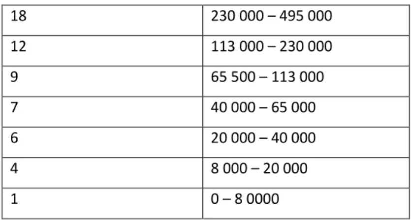
Therefore a set up based on the principals of the Wilson Formula but delimitated by the total number of goods receipt at the current work station was created. In figure V the logic behind the order quantities are described, the more stock value a material generates the more frequent it´s purchased.
Number of orders per year Value of annual usage (SEK)
22 18 230 000 – 495 000 12 113 000 – 230 000 9 65 500 – 113 000 7 40 000 – 65 000 6 20 000 – 40 000 4 8 000 – 20 000 1 0 – 8 0000
Figure V – Order quantity logic
But as this report is being written TSAB is changing their planning system and the new system will use the Wilson formula since the decision regarding maximum number of goods receipts has been re-evaluated and therefore the Wilson formula will be used in this report.
6.2.3 Service level (Availability)
The term service level is used to describe in what extent an item should be available on stock for a customer or, in the case for TSAB´s central warehouse in Lund, be available for stock refill and sales order. Of course a higher service level gives higher customer satisfaction but this must, as always, be taken into comparison with the cost associated with a higher service level in terms of higher stock value. Unfortunately it´s difficult to estimate what, if any, impact a changed service level has on the
experienced customer satisfaction. The service level determinates the safety stock and thereby the deviations that are permitted during an order cycle before a stock out situation occur.
There is actually a commonly used alternative way of looking at how to decide the safety stock, the cost of shortage. It´s based on calculating the cost of each shortage and minimizing the total cost with the shortage cost included and thereby set the
23
safety stock level. This method has an obvious problem, how is the shortage cost set? This is a problem which could ruin all further calculation if it´s not handled with care. As TSAB don´t use the shortage cost definition it will not be discussed further. When deciding the service level there is two main concepts, Serv1 or Serv2. Serv1: Probability of no stock out per order cycle.
Serv2: Fraction of demand that can be satisfied directly from stock on hand during a time period (note that it´s not during an order cycle).
The first service level concept is easier to use but is not as easy to translate to reality. The order quantity is not taken into consideration with the Serv1-concept and could give very misleading results. E.g. if the service level is 90% and the order quantity cover a full year of demand then there is a 10% statistical risk of getting a stock out during a year but if the order quantity cover only one week´s demand then there is a 1- = 99,6% risk of getting a stock out. In other words the service level needs to be higher for materials with short order cycles to keep the same service level. The level of Serv1 should thereby be defined according to the length of the order cycle and this makes it not as tangible as Serv2 which is easy translated to customer satisfaction, the fraction of customer orders will not be sent on time.
Assuming a normal distributed demand during the lead time the Serv1-concept could be calculated according to the cumulative distribution function for normal
distribution:
24
TSAB is using the Serv1-definition when sizing the safety stock and this could be questioned since most of the materials are being purchased several times a year, see figure V, and with the new planning system this is estimated to be even more
frequent since the Wilson-formula will be applied without the limitations of goods reception. Unfortunately this will decrease the availability according to above discussion if no adjustments to the service levels are made.
25
7. Empirical data
This chapter gives an insight in the data collection process, assumptions and limitations made regarding the input data of the calculations.
7.1 Data collection
The data collected for this report are mainly tied to one of two head categories, material data and transportation data. The material data is everything related to the characteristics of the materials analysed and are all extracted from the internal data analysing tool. Examining the materials extracted there are a lot of materials without standard deviation from the report, this is not a likely situation and when looking at the detailed information from the planning system it´s not confirming the strange observation at all, therefore all materials without standard deviation are overlooked. The other problem is the weight data, is it reliable? Many materials have the exact weight of 1 kg and other have no weight. Are these estimates or faulty standard values? In theses analysis they will be considered as correct.
While the material data is straight forward to collect, the transportation data is the opposite. The parameters have been collected from the local warehouses, the central warehouses and the freighters. The basic data regarding transportation cost and agreements were collected through the transportation organization at the central warehouses, in this data the transportation lead time and numbers of departures were included. The most complex data to collect was the local handling at the local warehouses. This process is not centrally controlled and therefore the variations are as many as the sites. All data has been collected through interviews with employees at the sites both regarding transportation costs and transport lead times. Several of the warehouses are not used to sea transportations and therefore no data in that field are available for those sites.
26
Apart from the two head categories described above there are data regarding financial and environmental aspects. The financial data was collected through
interviews with employees at the central warehouse and the environmental data was collected through interviews with employees at the transportation department at the central warehouse and through the webpage of NASDAQ’s CO²-emission trade.
7.2 Transportation cost
Tetra Pak AB (i.e. not only TSAB) has one global contract for both air and sea shipments for each site (although TSAB have set up a local agreement for air shipments to Dubai). The global contracts enable all Tetra Pak organizations to use the contract and the prices are negotiated on the total global volume. The global contract is an important parameter in the evaluation of transportation mode in this report since if the contract wouldn´t have been global the threshold of changing to sea shipments would have been completely different and the current favourable situation wouldn´t have been achieved. The sea contract is truly global since the price per kilogram is the same regardless of destination.
Compared to air freight that are able to ship each day of the week the sea shipments have fixed days in the months for departure which means that an extra stock needs to be included for the possibility that a need occurs outside the shipping dates. This could have been handled as a non constant lead time but due to low impact the deviations will instead be handled as a worst case scenario regarding lead time. Both air and sea transporters use what is called volumetric weight when calculating transportation fees. The volumetric weight is simply the volume of the goods converted to a weight by a predefined constant and then highest weight is used, e.g. if a shipment weigh 3 tonne and is 2 cubical meters large and the freighter uses a conversion constant of 2, then the volumetric weight is 4 tonne and the price is
27
defined as if the weight was 4 tonnes. Sea cargo is less dependent on weight and thereby the conversion constant used are higher.
When using sea freights there are two main concepts used, either LCL (less than container load) or FCL (full container load). The difference between the two concepts is that when using a LCL agreement the prices are defined per kilo and in a FCL agreement they are defined per container. Only the LCL concept will be considered in this report since the regular volumes doesn´t add up to even near a whole container with the current set up and restrains of this report.
7.3 The local sites
Below the situation regarding customs and local transportations are described for each of the local sites.
7.3.1 China
The warehouse in China is located in the harbour of Shanghai and being the world city it´s the infrastructure provides very good alternatives for both sea and air shipments. Due to the warehouse central location in the global Tetra Pak network they are used to handle both air and sea shipments at the site. The custom situation is good and the average customs time is not generally a problem. The local transportations are calculated per whole truck for sea shipments and at a fixed cost per shipment for air shipments but with a maximum of 2 tonnes.
7.3.2 Brazil
In Brazil the warehouse is located in the vicinity of Sao Paulo and the sea shipments through the harbour of Santos. The sea shipment conditions are good and the
warehouse is used to sea shipments but not in a wide extent. This causes the handling at custom to be experienced as longer and more complicated for sea shipments. The
28
general situation with customs is complex and there could be several days of delay. The fees for the local transports of the sea shipments are calculated per truck used and for air shipments a scaled cost model is used with a fixed price for certain weight intervals.
7.3.3 Mexico
The situation in Mexico is similar to the one in Brazil regarding local handling, both sites uses an agreement based on numbers of trucks for sea shipments and both have a set up with a fixed price for predefined weight intervals. The personnel in Mexico also stresses that the lesser experience of sea transportation makes the handling more complex due to the lack of relations and communication routes. Even the geographical setting is similar with the warehouse situated in Mexico City and the port of Veracruz as arriving port, even if the distance is somewhat longer.
7.3.4 United States
The warehouse in the United States is located in Chicago. This location creates some obvious questions regarding the sea shipments since Chicago is located far from the coast. In the agreement with the transporter the total transport time includes the train transportation from New York to Chicago. The warehouse in Chicago is not normally handling sea shipments and therefore no price list exist for this kind of local transports and in this report the cost is assumed equal to the local air shipment handling. For air shipment a flexible pricing model is used where the price is set per kilogram but with a scale system with more discounts the higher the total weight is. Chicago is facing a situation where 10-12 % of the shipments should be controlled and the time in custom could be almost two weeks.
29
7.3.5 United Arab Emirates
The last and most deviating set up is the one at the local warehouse in Dubai. TNT is responsible for the transport from the warehouse in Lund to the warehouse in Dubai, a door-to-door service. This is in a great extent possible due to the geographical vicinity between the airport and the TSAB warehouse in Dubai; they are situated in the same free trade zone. The price model is completely different from the one with Geodis Wilson and is based on different prices depending on each weight. I.e. there is fixed price for all shipments up to 11 kg and then there is a new fixed price for each whole kilogram added. In other words it´s the same price to send 31,2 kg as 31,9 kg. This price model has a non linear price evaluation, the heavier the shipment is the less the price per kilogram is. This creates some difficulties in the calculation since each shipment has a unique price per kilogram but in the report the price is based on the price per kilogram when sending a shipment of 100 kg. 100 kg is namely the average weight sent to Dubai between January and April in 2011. To make the calculations even more complex the fuel cost is added as a varying mark up but in this report the mark up from 2011-06-09 is used, 12,5 %. The warehouse is not used to handle sea transports and due to the location in harbour the local handling is disregarded in this report.
7.4 Sea transportation
7.4.1 To departing port
Geodis Wilson are responsible for the land transports from the warehouse in Lund to the departing port. The departing port is Gothenburg in all cases except Dubai where Malmö serves as outbound port. The transport to Gothenburg and Malmö are considered as one day since for sea shipments there is a last closing date (last date the goods should be at the port) that needs to be respected in order to be included at
30
the next shipment. The time from the closing date to departure varies in this report between 1-3 days.
7.4.2 Port to port
The price for all sea freights are the same unaware of the destination and the
volumetric conversion constant is that one tonne equals one square meter. In the sea freight agreement all shipments are calculated in whole tonne or square meters and for the calculations in this report that´s neglected but will be needed to taken into consideration in the conclusions. It should be noted that TSAB is in an extraordinary situation since their normal volumes wouldn´t be able to provide a contract as the one with Geodis Wilson but since other parts of Tetra Pak are using sea shipments to a great extent they are provided this opportunity.
In the sea freight agreement there is a price agreement but not a transit time
commitment for Dubai. The Dubai transit time has been based on an evaluation from Geodis Wilson and four departures per month are presumed to be available due to the large amount of shipments to Dubai. For all other sites both price and transport time is included in the agreement.
7.4.3 From arriving port
The transportation set up from the port to the local warehouse is handled locally by each market company and therefore there are as many set ups as there are market companies. When it comes to sea shipments neither Chicago nor Dubai had any experience and in this report their local transports regarding sea will be handled in the same way as their local air shipments.
For China, Brazil and Mexico the market companies are used to sea shipments but they could be that these very big shipments will be far greater than the potential
31
Technical Service volumes. For all three sites the price list from the port is set up per truck and not per kilogram. In this report the price per kilogram has been defined as the truck price for the trucks needed in aspect of the average bulk shipments first four months of 2011 divided by the total weight of those shipments.
7.5 Air transportation
Geodis Wilson also takes care of the most of the flight routes; once again it´s only Dubai that´s deviating in the report. The Dubai route is handled by TNT and has a special set up that will be handled below. The air transports are much more flexible and daily shipments are sent to all destinations in this report Monday to Friday for all destinations.
7.5.1 To departing port
As in the case with sea shipments the transporters are responsible for the transport from Lund to the airport and this transport is included in the price from port to port. But the transit time from Lund to departure are much shorter since the loading process are less complex and a shipment departs the same day as it´s shipped from Lund.
7.5.2 Port to port
The agreement with Geodis Wilson is based from the central warehouse to the arriving airport and consists of a fixed and a weight depending part. Apart from that there is a minimum fee charge but this will be disregarded since the volumes in scope for this report will generally not be affected by this fee. Furthermore both Mexico and Shanghai have a less flexible but more expansive route alternative that will not be considered in this report since it´s not commonly used with the current set up. A, in many ways different, set up is made with TNT where the agreement stretches from
32
door-to-door, i.e. TNT are responsible for the transport from the warehouse in Lund all the way to the warehouse in Dubai.
7.5.3 From arriving port
As in the situation with the local transportation from the port to the warehouse the airport transport have different setups at each site. These setups have been described in section 7.3.
7.6 Storage cost
TSAB uses a standard value of 20 % as stockholding cost and this standard value is used throughout this report. An additional parameter that indirectly affects the cost of storage is the cost per order for each site. It´s included together with the
stockholding cost in the calculation of ordering quantities. This data has been provided by the project that is currently implementing the new planning system for TSAB and is € 6 per order for all sites except Lund and Shanghai where it´s € 20 per order. The combination of the calculation of average stock, ordering quantity divided per two added by the safety stock, multiplied by the stockholding cost provides the annual storage cost.
7.7 Cost of capital
The cost of capital is also collected from the standards used within TSAB and the value used is 9 %.
7.8 Environmental cost
To measure the environmental impact of the transportation methods the amount of carbon dioxide emissions has been chosen. The two obvious problems with this method are how high the emissions are for the chosen way of transport and what cost is associated with the emissions. The cost of emissions is a difficult case to solve
33
and fluctuates in line with the political temperature. Many attempts have been made in this field but one the most widespread theory at the moment is the emission rights granted by the European Union. The cost of emission is in this model based on the cost level of this emission rights at the Nasdaq OMX commodities market, € 13/tCO2. The global transportation organization in Tetra Pak has together with NTM –
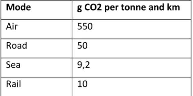
Nätverket för Transporter & Miljö calculated an average emission for each mode of transportation. The data is based upon a large database of real life measurements from transporters. Unfortunately it´s not specifically based on long distance flights and long distance sea shipments. Sea shipments could be argued to be less affected since the start up energy is much less dominant than in the case of flights and thereby the air rate could be modified to a lower value but this factor is not considered in this paper. The sea rate has been down scaled by Tetra Pak since the collaboration with NTM (previously 12). The detailed information could be found in figure VI. The sea and air distances in this report are provided from Geodis Wilson and the road and railroad distances are extracted with the assistance of Google´s distance provider. The ports in Chicago, Shanghai and Dubai and the distances from airports to warehouses are considered to be neglectable in terms of emissions.
Mode g CO2 per tonne and km
Air 550
Road 50
Sea 9,2
Rail 10
35
8. Analysis
8.1 The design of the experiment
To compare the two modes of transportation the first step is to create the formula for the total cost of the both alternatives. The formula for total cost demands all input data on a detailed level. To break this down to a simplified, easy to use formula, an experiment to analyse the detailed total cost formula is conducted and will finally give a “total gain formula” where a separate material could be entered and the (eventual) gain to change from air to sea transportation will be the result. I.e. the experiment should provide a simplified general formula based on analysis of the different affecting parameters and their impact. The first task is to identifying these affecting parameters.
The first interesting parameters are those of the materials since the analysis should be able to be performed for all types of materials, i.e. the parameters service level target, price, weight, volume, demand and standard deviation. The standard deviation is only interesting to look at in comparison to the demand and therefore a ratio between the demand and the standard deviation is used, which gives the volatility of the material.
Apart from the material parameters there are two interesting transportation parameters, the difference in price and transportation time in the both alternatives. The cost is only based on the varying part of the cost since the fixed cost is a very small part of the total picture and it´s difficult to analyse how this cost could develop. The last parameter that´s included is the environmental cost since this parameter could be calculated based on totally different approaches.
36
Below are a summary of the above mentioned affecting parameters in the total cost formula:
- Service level target - Price
- Weight - Volume - Demand
- Demand/standard deviation ratio - Environmental cost
- Transportation cost difference - Transportation time difference
These parameters will all be investigated further to see how they affect the gain of changing from air transportation to sea transportation. To do the analysis of each parameter a fixed high and low value are chosen for the four investigating parameters price, weight, standard deviation and demand (demand is only included in the last two analysis). I.e. each investigating parameter will be denoted high or low and this will generate a maximum a 64 materials. If there would have been only two
investigating parameters there would only have been generated four materials (H/H, H/L, L/H and L/L). In the below graphs there will be a maximum of eight materials simultaneously since a maximum of three investigating parameters will be used. The previously described affecting parameters are then simulated separately for all the, up to eight, materials by the use of the detailed formula. E.g. if the affecting
parameter service level target is to be analysed, first the material with high price, high weight and high standard deviation (demand will be investigated separately) is simulated in the formula with the service level ranging from a low value to a high
37
value. Then the procedure is repeated for the material with high price, high weight, and low standard deviation etc. These results will be displayed below.
Transportation cost and transportation time difference will also be investigated with demand as an parameter since they have not been included in the demand-graph, environmental cost, volume and service level target should also be analysed with demand but since they have an extremely low impact (see graphs below) this will be disregarded.
8.2 Results of the experiment
In the following graphs the result from the simulations of the model are presented. The graphs are built by series that are denounced in the format of X/X/X/X where the different letters stands for Price/Weight/Standard deviation/Demand, the last two from the central warehouse. The four parameters are divided into two levels each, either high or low, denounced as H or L. The graphs show the development of the gain when altering the chosen parameter. The gain is defined as the difference between the total cost of air transportation and the total cost of sea transportation.
In the graphs below it´s important to keep in mind that the sometimes extremely high values on gain could be misleading since all parameters are fictive.
38
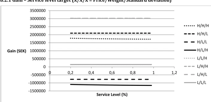
8.2.1 Gain – Service level target (X/X/X = Price/Weight/Standard deviation)
Figure VII – Gain – Service level graph
In figure VII it is clear that the impact of the service level at the central warehouse it´s obviously insignificant in the choice of transportation. But one interesting deviation to notify is the slight decrease of gain for higher service level at the material with high price and high standard deviation. Since high standard deviation increase the safety stock and high price increase the storage cost the decreased waiting time at the central warehouse, which follows from the increased service level, affect the total cost less for air shipments due to the square root in the safety stock calculation at the market company.
The two lines, L/H/H and L/L/H are almost entirely similar with line L/L/H and L/L/L so much that they are not visible in figure VII. Since the standard deviation primarily affects the safety stock it´s natural that materials with low price are very little affected by the change in standard deviation. This is because the safety stock in its
-1500000 -1000000 -500000 0 500000 1000000 1500000 2000000 2500000 3000000 3500000 0 0,2 0,4 0,6 0,8 1 1,2 Gain (SEK) Service Level (%) H/H/H H/H/L H/L/L H/L/H L/L/H L/H/H L/H/L L/L/L
39
turn affects the cost of storage which is an insignificant factor if the value of the goods is low. Not to surprisingly a high weight generates a higher gain since the transportation cost is increasing. And almost as unsurprisingly the lower price generates a higher gain due to the lower storage cost and cost of capital. Looking at the high price items it´s obvious that the change in standard deviation creates a change in gain. This is as mentioned due to the higher level of safety stock.
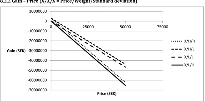
8.2.2 Gain – Price (X/X/X = Price/Weight/Standard deviation)
Figure VIII – Gain – Price graph
In figure VIII it´s very clear that a high price material is less profitable to ship by sea but apart from the obvious there are two observations. The materials with a high standard deviation have a faster decline in gain and this is due to the higher safety stock generated. Also noticeable is the higher starting point for the materials with
-70000000 -60000000 -50000000 -40000000 -30000000 -20000000 -10000000 0 10000000 0 25000 50000 75000 Gain (SEK) Price (SEK) X/H/H X/H/L X/L/L X/L/H
40
high weight. The higher weight increases the price possible without making it less profitable to ship the goods with sea shipments.
41
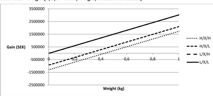
8.2.3 Gain – Weight (X/X/X = Price/Weight/Standard deviation)
Figure IX - Gain – Weight graph
The instinctive thought that heavy goods are well suitable for sea shipments are certified with above graph. The L/X/H and L/X/L are approximately the same and therefore the graph only seems to consist of three series. As stated in previous graphs a low cost item is more profitable to send by sea shipments and once again it´s viable that the standard deviation does not affect materials with a low cost significantly. Also further confirmed is the statement that high price items have more to gain if they have a low standard deviation.
-2500000 -1500000 -500000 500000 1500000 2500000 3500000 0 0,2 0,4 0,6 0,8 1 Gain (SEK) Weight (kg) H/X/H H/X/L L/X/H L/X/L
42
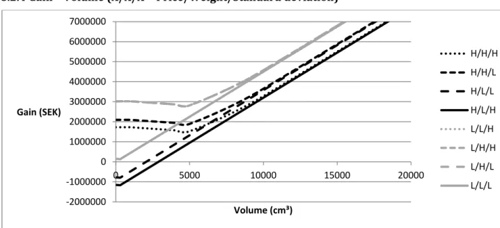
8.2.4 Gain – Volume (X/X/X = Price/Weight/Standard deviation)
Figure X – Gain – Volume graph
The volume of the material only affects the transportation cost and only interferes when the volumetric weight exceeds the normal weight. Looking closer at the data behind the graph all series starts with a constant phase which ends when the volumetric weight for sea shipments exceeds the weight of the material. The following declining phase, most viable for the high weight materials, is the result of the volumetric weight increasing for sea shipments and the air shipments still being constant since the normal weight has not been exceeded. The third phase starts when the volumetric weight for air shipments is exceeded and then the higher cost for air shipments is dominating the cost and makes the gain for sea shipments increase rapidly.
As seen in the other graphs the materials with a low price are indifferent in respect to the standard deviation and this explains the “absence” of series L/H/H and L/L/H.
-2000000 -1000000 0 1000000 2000000 3000000 4000000 5000000 6000000 7000000 0 5000 10000 15000 20000 Gain (SEK) Volume (cm³) H/H/H H/H/L H/L/L H/L/H L/L/H L/H/H L/H/L L/L/L
43
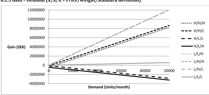
8.2.5 Gain – Demand (X/X/X = Price/Weight/Standard deviation)
Figure XI - Gain – Volume graph
Figure XI is a good display of what materials those are profitable to send by sea shipments since the higher demand the more obvious it´s that if the material is suitable. As in many of the previous graphs there are very little difference between both materials L/H/H and L/H/L and also between materials L/L/H and L/L/L,
therefore it seems to be only six series. The conclusion of this graph is very clear and confirms the intuitive feeling that a high weight and low value article is the most interesting items for sea freight and that high price and low weight items are the most interesting for air shipments. Then the difference in standard deviation only excels the result as well as the increasing demand.
-4000000 -2000000 0 2000000 4000000 6000000 8000000 10000000 12000000 0 10000 20000 30000 40000 50000 Gain (SEK) Demand (Units/month) H/H/H H/H/L H/L/L H/L/H L/L/H L/H/H L/H/L L/L/L
44
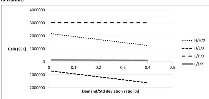
8.2.6 Gain – Demand/Std deviation ratio (X/X/X = Price/Weight/Standard deviation)
Figure XII - Gain – Demand/Std deviation graph
Figure XII is a very obvious result that the weight does not affect the gain of an increasing standard deviation compared to the demand. Looking at the background it´s not unexpected to have these results since the increased standard deviation increases the safety stock and the safety stock affects the storage cost together with the material price. In other words all materials will be more suitable to send by air shipments with a higher standard deviation but the difference is increasingly significant for high price articles.
-2000000 -1000000 0 1000000 2000000 3000000 4000000 0 0,1 0,2 0,3 0,4 0,5 Gain (SEK)
Demand/Std deviation ratio (%)
H/H/X H/L/X L/H/X L/L/X
45
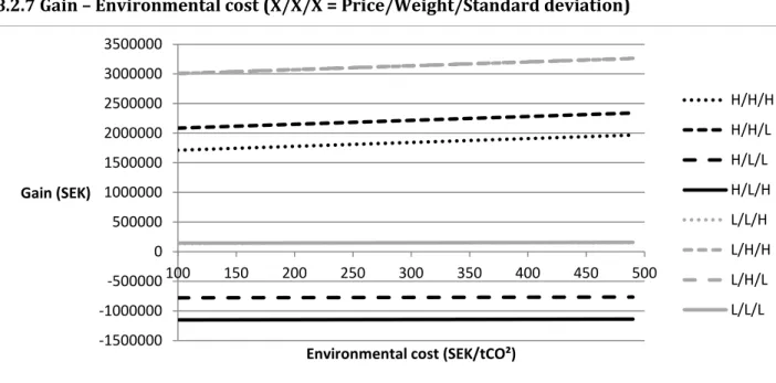
8.2.7 Gain – Environmental cost (X/X/X = Price/Weight/Standard deviation)
Figure XIII – Gain – Environmental cost graph
The cost of the environmental impact is very difficult to assess and of course the gain of sea shipments increase more rapidly for a heavy material then for a light one but the important observation is that not even for a high weight material the impact of a four doubled environmental cost the result is drastically changed.
-1500000 -1000000 -500000 0 500000 1000000 1500000 2000000 2500000 3000000 3500000 100 150 200 250 300 350 400 450 500 Gain (SEK)
Environmental cost (SEK/tCO²)
H/H/H H/H/L H/L/L H/L/H L/L/H L/H/H L/H/L L/L/L
46
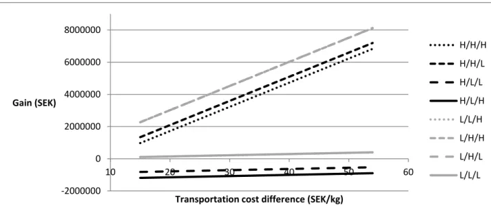
8.2.8 Gain – Transportation cost difference (X/X/X = Price/Weight/Standard deviation)
Figure XIV - Gain – Transportation cost difference graph
Clearly displayed in the above graph is that the difference in transportation cost mainly affects materials with high weight. The higher the price is the less gain is sustained through sea shipments.
-2000000 0 2000000 4000000 6000000 8000000 10 20 30 40 50 60 Gain (SEK)
Transportation cost difference (SEK/kg)
H/H/H H/H/L H/L/L H/L/H L/L/H L/H/H L/H/L L/L/L
47
8.2.9 Gain – Transportation time difference (X/X/X = Price/Weight/Standard deviation)
Figure XV - Gain – Transportation time difference graph
Transportation time to sea is affecting the cost of capital during the transportation and the storage cost at the market company since the lead time is prolonged and an additional safety stock is needed. With this in mind the weight of the material should not affect the gain when altering the transportation time which also could be read from the graph since the series with diverting weights are parallel.
Looking at the series with equal cost and weight the series with high standard deviation have a slightly faster decline than the one with a low standard deviation. This is due to the higher uncertainty during the transportation which will be needed to take into consideration at the safety stock. Looking at the series with the same weight and standard deviation shows a large impact from the price. The gain declines clearly with a higher price due to the increased cost of capital and storage cost.
-3000000 -2000000 -1000000 0 1000000 2000000 3000000 4000000 10 15 20 25 30 35 40 45 50 Gain (SEK)
Transportation time difference (Days)
H/H/H H/H/L H/L/L H/L/H L/L/H L/H/H L/H/L L/L/L
48
8.2.10 Gain – Transportation cost difference, demand included (X/X/X/X = Price/Weight/Standard deviation/Demand)
Figure XVI - Gain - Gain – Transportation cost difference graph (Demand included)
The graph shows that the transportation cost becomes a dominant figure when the air rate is increasing. The series with low weight items are not at all affected in the same extent that the high weight items and comparing the different demand types shows that a higher demand affects the increase more than a low demand.
-50000 0 50000 100000 150000 200000 250000 300000 10 15 20 25 30 35 40 45 50 Gain (SEK)
Transportation cost difference, demand included (SEK/kg)
X/H/X/H X/H/X/L X/L/X/H X/L/X/L
49
8.2.11 Gain - Transportation time difference, demand included (X/X/X/X = Price/Weight/Standard deviation/Demand)
Figure XVII - Gain – Transportation time difference graph (Demand included)
In figure XVII the materials are divided into two major groups, high demand and low demand items. High demand items have a clearly higher decrease level. In both groups there are two items, low cost items, which are almost not affected by the raised transportation time at all. The high cost items on the other hand have different decrease level depending on the standard deviation, high standard deviation equals high decrease.
8.2.12 Summary of the graphs
The observations from the graphs provide the data to generate a specific equation for the transportation decision. Since the impact from service level at the central
warehouse and from the environmental cost is quite insignificant these parameters will not be taken into consideration in the model. It´s also assumed that most
-20000 0 20000 40000 60000 80000 100000 120000 140000 10 15 20 25 30 35 40 45 50 Gain (SEK)
Transportation time difference, demand included (Days)
H/X/H/L H/X/L/L H/X/H/H H/X/L/H L/X/H/L L/X/L/L L/X/H/H L/X/L/H
50
material have a larger weight than volume impact and therefore the volume aspect is overlooked.
The two graphs describing the full situation are figure XVI and XVII. Since the only parametrical differences between shipping by air and sea are the transportation time and the transportation cost. Furthermore there is the environmental impact as well but since it was shown in the above graphs that the effect was minor in terms of tangible costs it will be overlooked.
Gain – Transportation cost difference, demand included: Gain – Transportation time difference, demand included:
51
52 Combined:
To calculate the total gain when changing all parameters the two equations needs to be combined. The only parameters used in both equations are the demand. In g(x) the demand affects everything except a constant. The constant is equal to the collected expression from h(y) which don´t include the demand as a parameter. Comparing the remaining equations, where demand is affecting everything and could be broken out, there are two more single constants which could be replaced by the out broken expression from the other equation. The result looks like this with some rounded values:
53