SSM’s external experts’ review of
SKB’s safety assessment SR-PSU
– consequence analysis
Main review phase
SSM perspective
BackgroundThe Swedish Radiation Safety Authority (SSM) received an application
for the expansion of SKB’s final repository for low and intermediate level
waste at Forsmark (SFR) on the 19 December 2014. SSM is tasked with
the review of the application and will issue a statement to the
govern-ment who will decide on the matter. An important part of the
applica-tion is SKB’s assessment of the long-term safety of the repository, which
is documented in the safety analysis named SR-PSU.
Present report compiles results from SSM’s external experts’ reviews of
SR-PSU during the main review phase. The general objective of these
reviews has been to give support to SSM’s assessment of the license
application. More specifically, the instructions to the external experts
have been to make an in depth assessment of the specific issues defined
for the different disciplines.
Project information
Contact person SSM: Georg Lindgren
Table of Contents1) SR-PSU Main Review Phase: Radionuclide Transport Modelling
George Towler and James Penfold
2) Review of Initial State and Process Reports for Waste, Barriers,
and Geosphere
Richard Metcalfe
3) Consequence analysis review: importance of caissons in 2BMA
George Towler and James Penfold
4) Review of specific topics relating to the biosphere dose assessment
for key radionuclides
2017:30
SSM’s external experts’ review of
SKB’s safety assessment SR-PSU
– consequence analysis
This report concerns a study which has been conducted for the
Swedish Radiation Safety Authority, SSM. The conclusions and
view-points presented in the report are those of the author/authors and
do not necessarily coincide with those of the SSM.
Authors:
George Towler and James Penfold
1) 1)Quintessa Limited, Henley on Thames, UKSR-PSU Main Review Phase:
Radionuclide Transport
Modelling
Activity number: 3030014-1020
Registration number: SSM2016-3260 Contact person at SSM: Shulan Xu
1
Abstract
The Swedish Radiation Safety Authority (SSM) received an application for the expansion of SKB’s final repository for low and intermediate level waste at Forsmark (SFR) on the 19 December 2014. SSM is tasked with the review of the application and will issue a statement to the government who will decide on the matter. An important part of the application is SKB’s assessment of the long-term safety of the repository, which is documented in the safety analysis named SR-PSU.
SSM’s review is divided into an initial review phase and a main review phase. This assignment contributes to the main review phase. It involves re-implementing SKB’s radionuclide
transport models for two of SFR’s vaults (1BMA and 2BMA), and the geosphere, in a suitable compartmental modelling code; and then comparing the results with the results of SKB’s models.
The comparison exercise was undertaken using information and data from SKB’s SR-PSU reports; additional information provided by SKB at a meeting between SKB, SSM and supporting consultants held on 28th April 2016; and SKB’s model input and data files, which
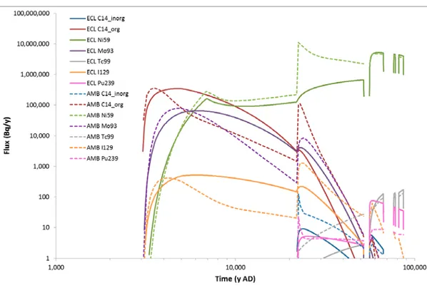
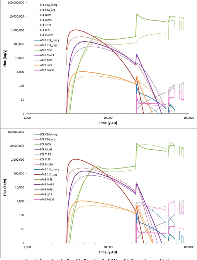
were supplied in October 2016. SKB implemented their models using the ECOLEGO code. The models developed as part of the comparison exercise were implemented using the AMBER code. The findings of the model comparison exercise are summarised as follows. SKB have built a detailed and complex model of radionuclide transport through the 1 BMA and 2BMA vaults into the geosphere. SKB have put significant effort into representing the detailed geometry of the near-field, spatial variations in near-field flows, and evolution of the system in response to environmental change and barrier degradation. SKB’s reports provide a high level description of the models, which enable the configuration to be broadly understood or deduced. However, description of the representation of the different waste package types in the models could be improved, and some aspects of the model configuration are not described, for example how the waste packages and caissons have been discretised.
The models use a large amount of data. Most of these data are provided in SKB’s reports, but not all; for example the properties of the waste packages (porosity, density, effective
diffusivity, etc) and the detailed flows through the vaults are not presented. (The latter were provided in spreadsheets by SKB). A potentially significant observation is that 2384 steel drums containing cement embedded wastes are planned for disposal in the 2BMA vault, but no inventory is assigned to these drums in SR-PSU. This means that the inventory of 2BMA could be under estimated, and consequently so could the flux of radionuclides released from the vault.
SKB have not described and justified how key aspects of the model have been parameterised, where the parameter values are derived from the underpinning data. This includes important parameters such as cross-sectional areas and distances used to calculate diffusive transfers. Although SKB’s documentation of the model and data could be improved we have built a model in AMBER that broadly reproduces the results of SKB’s ECOLEGO model for the 2BMA vault. This helps to build confidence in SKB’s assessment calculations for SR-PSU. However, the differences are such that SSM might wish to consider further work to investigate these differences in more detail.
SKB’s geosphere model also contains a large number of compartments, but it is less complex than the models of the vaults, and documentation of the model is more complete and
with only small differences that can be attributed to the coarser discretisation of the AMBER model compared with the ECOLEGO model.
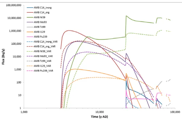
Due to the complexity of SKB’s models, and limitations in their documentation, it was not possible to undertake the high level comparison exercise for 1BMA that was originally planned by SSM. Instead efforts focussed on analysing a range of base case model results, and results from variant cases, to help understand the behaviour of the 2BMA vault model, and the reasons for differences in the fluxes calculated by the AMBER and ECOLEGO models. The key areas for further investigation have been successfully identified and are described in the conclusions section of this report. Once this further investigation has been completed, it should be
relatively efficient to use the AMBER model to further explore the radionuclide transport behaviour, including undertaking a high level comparison exercise for 1BMA.
During the initial review phase, we undertook a high-level assessment of SKB’s identification of FEPs and their treatment in the assessment. We identified the key FEPs and associated uncertainties that are most significant for potential impacts are the radionuclide inventory and FEPs relating to the performance and degradation of the near-field engineered barriers. It was noted that understanding the coupled processes leading to degradation of the engineered barriers, the rate and timing of degradation, and selection of parameters to represent these processes in models are important. These issues are being considered by other technical areas within this main review phase. Nevertheless, the results of this modelling exercise further highlight the importance of these issues.
Further analysis of SKB’s identification and treatment of FEPs, in the context of radionuclide transport, was undertaken as part of this main review phase. Given the knowledge gained during the initial review phase, and during the review of the initial state and process reports, the FEPs represented explicitly in the radionuclide transport models were found to be consistent with expectations. The FEPs represented explicitly are also broadly consistent with safety assessments undertaken for similar facilities, and have been represented using
appropriate mathematical models. No omissions of further issues were identified beyond those raised by the initial review and the subsequent further analysis of SKB’s identification and treatment of FEPs.
with only small differences that can be attributed to the coarser discretisation of the AMBER model compared with the ECOLEGO model.
Due to the complexity of SKB’s models, and limitations in their documentation, it was not possible to undertake the high level comparison exercise for 1BMA that was originally planned by SSM. Instead efforts focussed on analysing a range of base case model results, and results from variant cases, to help understand the behaviour of the 2BMA vault model, and the reasons for differences in the fluxes calculated by the AMBER and ECOLEGO models. The key areas for further investigation have been successfully identified and are described in the conclusions section of this report. Once this further investigation has been completed, it should be
relatively efficient to use the AMBER model to further explore the radionuclide transport behaviour, including undertaking a high level comparison exercise for 1BMA.
During the initial review phase, we undertook a high-level assessment of SKB’s identification of FEPs and their treatment in the assessment. We identified the key FEPs and associated uncertainties that are most significant for potential impacts are the radionuclide inventory and FEPs relating to the performance and degradation of the near-field engineered barriers. It was noted that understanding the coupled processes leading to degradation of the engineered barriers, the rate and timing of degradation, and selection of parameters to represent these processes in models are important. These issues are being considered by other technical areas within this main review phase. Nevertheless, the results of this modelling exercise further highlight the importance of these issues.
Further analysis of SKB’s identification and treatment of FEPs, in the context of radionuclide transport, was undertaken as part of this main review phase. Given the knowledge gained during the initial review phase, and during the review of the initial state and process reports, the FEPs represented explicitly in the radionuclide transport models were found to be consistent with expectations. The FEPs represented explicitly are also broadly consistent with safety assessments undertaken for similar facilities, and have been represented using
appropriate mathematical models. No omissions of further issues were identified beyond those raised by the initial review and the subsequent further analysis of SKB’s identification and treatment of FEPs.
Contents
1 Introduction ... 5
2 Near-Field Model for 2BMA Vault ... 6
2.1 Model Configuration ... 6
2.1.1 Wastes ... 6
2.1.2 Barriers ... 9
2.2 Processes ... 14
2.3 Data ... 16
2.3.1 Radionuclide Decay Chains and Half-lives ... 16
2.3.2 Inventory ... 17
2.3.3 Waste Package Dimensions ... 19
2.3.4 Vault and Caisson Dimensions ... 20
2.3.5 Time Periods ... 21
2.3.6 Material Properties ... 23
2.3.7 Flows ... 25
2.3.8 Sorption and Solubility Limitation ... 29
3 Geosphere Model ...32 3.1 Model Configuration ... 32 3.2 Processes ... 34 3.3 Data ... 34 4 Calculation Cases ...37 5 Results ...44 5.1 Base Case ... 44
5.2 NF_Var1: Increased Discretisation of the Wastes ... 48
5.3 NF_Var2: Linear Interpolation of Flows ... 49
5.4 NF_Var3: No Diffusion, Advection Only... 50
5.5 NF_Var4: No Advection, Diffusion Only ... 51
5.6 NF_Var5: Progressive Fracturing of Structural Concrete ... 52
5.7 NF_Var6: No Fracturing of Structural Concrete ... 54
5.8 NF_Var7: Properties of the Wastes ... 55
5.9 NF_Var8: Cross-sectional areas for diffusive transport ... 55
5.10 NF_Var9: Simplified Model ... 56
5.11 NF_Var11: Probabilistic Case ... 58
5.12 NF_Var12: Representation of the Caisson Walls ... 61
5.13 NF_Var13: Combination of Changes ... 62
5.14 GEO_VAR1: Input of ECOLEGO Near-field Fluxes into AMBER Geosphere ... 62
6 Conclusions ...63
1 Introduction
The Swedish Radiation Safety Authority (SSM) has received an application for the expansion of SKB’s final repository for low and intermediate level waste at Forsmark (SFR) on the 19 December 2014. SSM is tasked with the review of the application and will issue a statement to the government who will decide on the matter. An important part of the application is SKB’s assessment of the long-term safety of the repository, which is documented in the safety analysis named SR-PSU.
SSM’s review is divided into an initial review phase and a main review phase. This assignment contributes to the main review phase. In the initial review phase, a number of specific topics for further in-depth review have been identified. The scope of those topics has been refined following SKB’s provision of complementary information, requested by SSM during the initial review phase and discussed at a meeting between SSM, SKB and supporting consultants on the 28th April 2016.
SSM wish to further understand and build confidence in the radionuclide transport calculations undertaken by SKB. To achieve this, SSM have identified four tasks.
1. To re-implement SKB’s radionuclide transport model for the 2BMA vault in a suitable compartmental modelling code. The model should use the same compartmental configuration as SKB’s model. The focus should be on review of the configuration of the assessment model to represent the conceptual model, linked to the choice of parameterisation. The model results should be compared to SKB’s results to build confidence that they are reasonable and to confirm there are no significantly anomalous behaviours. However, the aim is not to exactly reproduce SKB’s results. The model will also be used to test sensitivity of the results to the number of realisations and numerical seed, to build confidence that the number of realisations used by SKB should result in model convergence.
2. The geosphere is to be added to the near-field model developed in (1). Again the focus should be on review of the configuration of the assessment model to represent the conceptual model, linked to the choice of parameterisation. The model results should be compared to SKB’s results to build confidence that they are reasonable and to confirm there are no significantly anomalous behaviours. However, the aim is not to exactly reproduce SKB’s results. The model will also be used to test sensitivity of the results to the number of realisations and numerical seed, to build confidence that the number of realisations used by SKB should result in model convergence.
3. The model developed in (1) should be used to build confidence in SKB’s results for the 1BMA vaults. This will be achieved by changing the inventory and flows for those in 1BMA. SKB’s models for 1BMA and 2BMA have different compartmental configurations. Therefore, some pre-processing of the flows may be required and the model is not expected to exactly reproduce SKB’s results. However, the model results should still be sufficient to highlight any potential issues for discussion with SKB. 4. The model developed in the previous steps should be used to test sensitivity of the
results to any potentially important alternative assumptions that are identified during the course of the review.
Approach
The tasks specified by SSM have been undertaken by re-implementing SKB’s models in Version 6.0 of the AMBER code (Quintessa, 2016). The configuration and parameterisation of
the AMBER models is described in Sections 2 and 3 of this report, with reference to the SKB reports that describe the SR-PSU models, which were implemented using the ECOLEGO code. Section 4 describes the calculation cases that have been assessed using the AMBER model, and any calculation case specific data. Section 5 describes SKB’s results and compares these to the AMBER model results. Important assumptions and limitations to be noted by SSM are highlighted, as are any differences in the model results that may be important for safety. Section 6 concludes on the overall findings of the work.
During the initial review stage it was identified that some of information required to undertake these tasks is not directly available from SKB’s reports. Further information and clarifications were provided by SKB during the meeting of 28th April 2016, and a general information
request was also issued to SKB following the meeting. In response, part way through this main review phase, some additional data was provided by SKB including ECOLEGO model files and associated data input files in MS Excel. The ECOLEGO model and input data files have been used to fill some key information gaps. However, due to the size and complexity of the models, it was not practicable to compare and contrast every aspect of the configuration and parameterisation of the AMBER and ECOLEGO models.
2 Near-Field Model for 2BMA Vault
2.1 Model Configuration
2.1.1 Wastes
The 2BMA vault contains the following waste packages: Cement solidified wastes in concrete moulds. Concrete embedded wastes in concrete moulds. Cement solidified wastes in steel moulds. Concrete embedded wastes in steel moulds. Concrete embedded wastes in steel drums.
The numbers of waste packages associated with each waste stream is described in Appendix A of TR-14-02. This has been used to calculate the number of packages of each type in 2BMA (Table 1). It is noted that tetramoulds are included under steel moulds (p197 in TR-14-09). Table 1. Number of waste packages in 2BMA
Package Type Number
Cement solidified wastes in concrete moulds 192 Concrete embedded wastes in concrete moulds 967 Cement solidified wastes in steel moulds 68 Concrete embedded wastes in steel moulds 2225 Concrete embedded wastes in steel drums 2384
Section 9.3.10 in TR-14-09 describes the configuration of the near-field model to represent the different waste packages (Table 2). It is noted that no account is taken of the barrier provided
by the steel containers. This is likely to be a cautious assumption because the containers will be a barrier to release of radionuclides until they become significantly perforated by corrosion. The associated waste streams have been identified from Appendix A in TR-14-02 and the descriptions of the waste given in Section 9.3.10 in 14-01. It is noted that Figure 9-8 in TR-14-09 shows there are no bitumen solidified / embedded wastes in 2BMA.
Table 2. Configuration of the near-field model to represent the different waste packages (Section 9.3.10 in TR-14-09)
Package Representation Waste Types
Cement-solidified or concrete embedded waste in concrete moulds
This model waste package is represented using three
compartments, two for the interior with cement solidified or concrete embedded waste and one for the concrete mould. Solidified R.29 Embedded C.23, O.23/O.23:9, S.23, S.23:D Cement-solidified or concrete embedded waste in steel moulds
This model waste package is represented with two compartments for the interior with cement solidified or concrete embedded waste. The steel casing is not accounted for in the modelling. Solidified R.15 Embedded B.23:D, B.23:D.sec, C.4K23:D, F.23, F.4K23:D, F.4K23C:D, O.4K23:D, O.4K23C:D, O.4K23S:D, R.23, R.23:D, R.4K23:D, R.4K23C:D, Å.4K23:D, Å.4K23C:D Cement-solidified or concrete embedded waste in steel drums
This model waste package is represented with two compartments for the interior with cement
conditioned waste, the steel casing is not accounted for in the modelling.
Solidified None Embedded S.25D
Figure 1 shows the configuration of the AMBER model to represent the different wastes packages, as described in Table 2. The waste compartments are coloured red. The mould compartment is coloured dark grey, and the compartment representing the grout surrounding the waste packages is coloured light grey. Transfers between the compartments are shown in white. Forwards and backwards transfers are used in each case in order to represent migration of radionuclides by diffusion and advection. (Representation of transport processes is described later).
The 2BMA vault contains 14 caissons. Figure 1 shows the model configuration used to represent the waste packages in one caisson, plus the surrounding grout. The same configuration is used to represent the waste packages in each of the other thirteen caissons. Therefore, a total of 6 x 14 = 84 compartments are required to represent the waste packages.
Figure 1. Configuration of the AMBER model to represent the different waste package types
During inspection of the ECOLEGO model files, it was identified that the configuration of the compartments used to represent the waste packages had been misunderstood from the
description given in Section 9.3.1 of TR-14-09. In the ECOLEGO model, each package type is represented by two compartments: an inner waste compartment and an outer waste
compartment. The concrete moulds associated with cement solidified waste and cement embedded wastes are represented separately. This is illustrated in Figure 2. Therefore, for each of the 14 caissons there are the following additional waste package compartments compared with the AMBER model:
An additional waste compartment for each of the 5 package types.
An additional compartment to represent the moulds associated with cement solidified and concrete embedded wastes separately.
Therefore there are an additional 6 x 14 = 84 waste package compartments compared with the AMBER model. It was decided not to include these additional compartments in the AMBER model, but instead test sensitivity of the calculated fluxes to the discretisation of the waste packages for one caisson as a variant calculation.
2.1.2 Barriers
The 14 concrete caissons in the 2BMA vault are illustrated in Figure 3. Each caisson is surrounded by crushed rock backfill (macadam), including between the caissons. Macadam is also used to backfill the loading area (the right hand end of the vault in Figure 3) and the far end of vault (the left hand end of the vault in Figure 3). The waste packages are cement grouted into each concrete caisson.
Figure 3. 2BMA Vault (Figure 9-7 in TR-14-09)
Figure 4 shows the conceptual model for a single caisson. Radionuclides are transported out of the waste packages and through the near-field barriers by advection and diffusion. Transport from the macadam into fractures in the rock is only by advection.
Figure 4. Conceptual model of the 2BMA vault (Figure 9-8 in TR-14-09)
Section 9.3.4 in TR-14-09 states that each caisson is represented separately in the radionuclide transport model. For each caisson, the model also includes a compartment for macadam backfill surrounding the caisson. The macadam backfill in the ends of the vaults is also represented by one compartment for each end. Section 9.3.2 in TR-14-09 notes, “in the
radionuclide transport model, all outer walls were represented by five compartments each”.
At the meeting on 28th April 2016, SKB clarified that in the 2BMA vault model the caissons
are each represented by 5 radial compartments, whereas in 1BMA vault model, each wall of a caisson is subdivided into 5 compartments (i.e. a total of 30 compartments). The thickness of each of the five radial compartments used to represent the walls of the caisson is not described in the SR-PSU reports, so we have assumed each compartment represents the same thickness of concrete.
At the 28th April meeting SKB also noted that a single compartment is used to represent the
rock surrounding the 2BMA vault. Inspection of the ECOLEGO model files clarified that the rock surrounding the vault is represented by the first compartment of the geosphere model for transport through fractures in the rock. There is no compartment representing the specific volume of rock surrounding the vault.
The configuration of the compartments representing the near-field barriers is shown in Figure 5. The implementation in AMBER is shown in Figure 6 for a single caisson. The same
configuration is used for all 14 caissons. The colours of the compartments correspond to Figure 5, and transfers are shown in white. Forwards and backwards transfers are used to represent advection and diffusion of radionuclides through the near-field barriers, include transport along the length of the vault into the macadam surrounding adjacent caissons. There is only a single (forwards) transfer into rock, as only advection into the rock is represented in the model.
Figure 5. Configuration of compartments representing the near-field barriers
Figure 5. Configuration of compartments representing the near-field barriers
Figure 6. Configuration of the AMBER model to represent a single caisson
Figure 7 shows the configuration of the AMBER model to represent the 14 caissons and the macadam at the ends of the vaults. Transfers are used to represent advection and diffusion of radionuclides along the length of the vault, and advection into the rock. There is advection from the macadam associated with each caisson into the rock, and from the macadam at the ends of the vault into the rock. Therefore the model is able to represent transport parallel and perpendicular to the length of the vault. In total the 2BMA AMBER model comprises 198 compartments. The ECOLEGO model has an additional 84 compartments that provide a more detailed discretisation of the waste packages.
Fi gu re 7. C on fig ura tio n of th e A M B E R m od el to rep res en t t he 1 4 ca iss on s (b lu e) an d m aca da m a t t he en ds o f t he v au lt (y el lo w )
Fi gu re 7. C on fig ura tio n of th e A M B E R m od el to rep res en t t he 1 4 ca iss on s (b lu e) an d m aca da m a t t he en ds o f t he v au lt (y el lo w )
Conceptually the AMBER model is orientated with the x direction parallel to the long-axis of the vault, and the y direction (sideways) and z direction (vertical) perpendicular to the long-axis of the vault. Given the radial geometry of the
compartments used to represent the caissons and macadam, the vault was considered to be symmetrical about the x-z and x-y planes.
Due to the radial configuration, only a single set of transfers is required to represent transport from the waste packages, to the grout, through the caisson and into the backfill, i.e. separate sets of transfers are not required for each of the x, y and z directions. Two sets of transfers are required to represent transport parallel to the long-axis of the vault through the backfill, and perpendicular to the long-axis, from the backfill into the rock.
2.2 Processes
The key processes represented in the near-field model are: Decay and ingrowth of radionuclides.
Advection of radionuclides with groundwater. Diffusion of radionuclides in groundwater. Sorption of radionuclides.
Section 9.3.1 in TR-14-09 notes that solubility limitation is not considered in the main calculation cases.
Decay and ingrowth of radionuclides was calculated using the in-built functionality in AMBER. Transport of radionuclides, taking into account the effects of sorption, was calculated using the standard mathematical models:
Advection
C
Q
Whereλ is the transfer rate (y-1)
Q is the volumetric flow rate (m3 y-1)
C is the element specific capacitance (m3, Equation 9-6 in TR-14-09).
Diffusion
C
A
D
e
Whereλ is the transfer rate (y-1)
De is the effective diffusivity (m2 y-1)
C is the element specific capacitance (m3, Equation 9-6 in TR-14-09).
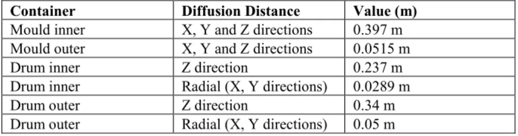
Δ is the distance from the mid-point of the compartment to the mid-point of the adjacent compartment.
Advection was represented using forwards transfers, while diffusion was represented using pairs of forwards and backwards transfers. This is the standard approach for compartmental models, as used in SKB’s models implemented using ECOLEGO. The calculation of distance from the mid-point of a compartment to the outer edge of
a compartment is illustrated in Figure 8 for the different waste types and near-field barriers. For the walls of the concrete moulds (not illustrated) the distance from the mid-point of the compartment to the outer edge of the compartment is equal to half the wall thickness.
Note the distance and cross-sectional area for diffusion are direction dependent and this must be accounted for when calculating the transfer rates. The AMBER model was configured such that different areas and distances can be specified in the x (parallel to the long axis of the vault), y (sideways) and z (up and down) directions. For simplicity, the different thicknesses of macadam above and below the caissons were not represented in the model, as this reduces the number of transfers that have to be included in the model and parameterised. This is not expected to have an important impact on the results, as advection by groundwater is always significant component of radionuclide transport through the macadam.
For radial geometry compartments, such as those used to represent the caissons, the cross-sectional area of the compartment, which is used in the diffusion calculations, was specified based on the dimensions of the outside of the compartment. However, in the transport calculations, the interface area between the compartments was always used. Therefore, while the cross-sectional area of the donor compartment was used for transfers away from the wastes, for backwards diffusive transfers towards the waste, the cross-sectional area of the receptor compartment was used. It is not clear if this distinction was made in SKB’s model – see equation 9-9 in TR-14-09.
In the AMBER model, the harmonic mean effective diffusivity was calculated for each diffusive transfer:
r e r d e d r d h e
D
D
D
, , ,
WhereDe is the effective diffusivity (m2 y-1)
Δ is the distance from the mid-point of the compartment to the mid-point of the adjacent compartment (m).
h is the harmonic mean d is the donor compartment r is the receptor compartment
Figure 8. Calculation of the distance from the mid-point of a compartment to the outer edge of a compartment
2.3 Data
2.3.1 Radionuclide Decay Chains and Half-lives
Table 3-1 in TR-14-09 describes the radionuclide decay chains and Tables A-3 and A-4 of the same report describe the half-lives. Only those radionuclides, and their progeny, that lead to the greatest radiotoxicity of releases from the near-field and geosphere have been included in the AMBER model. From Figure 5-1 and 5-2 in TR-14-09 these are:
C-14_inorg C-14_org Ni-59 Ra-226
Mo-93 Tc-99 Ag-108m I-129 Ac-227 Pa-231 U-235 U-238 Pu-239 Pu-240 Am-241 Am-243
2.3.2 Inventory
The numbers of packages of each type in 2BMA is given in Table 1. The total inventory in 2BMA is given in Table A-1 in TR-14-09. The inventory associated with each waste type was provided by SKB in an Excel spreadsheet1. The inventory
associated with each package type was calculated using the mapping between package type and waste type described in Table 2. When the inventory for each package type was summed, the total inventory was found to match that in Table A-1 in TR-14-09, except for Mo-93 where the calculated inventory was slightly higher than given in TR-14-09 and for U-235 where the calculated inventory was slightly lower. The inventory associated with each package type is given in Table 3. Table 3. Inventory in the different package types (Bq)
Cement solidified wastes in concrete moulds Cement embedded wastes in concrete moulds Cement solidified wastes in steel moulds Cement embedded wastes in steel moulds Cement embedded wastes in steel drums Ac-227 0.00E+00 0.00E+00 0.00E+00 0.00E+00 0 Ag-108m 2.34E+06 9.53E+08 3.26E+08 3.94E+10 0 Am-241 5.01E+06 1.20E+10 7.68E+08 2.85E+10 0
Am-242m 8.97E+03 2.22E+07 1.35E+06 1.60E+08 0 Am-243 3.44E+04 8.70E+07 5.65E+06 5.70E+08 0 Ba-133 1.66E+04 1.36E+07 1.33E+06 1.28E+08 0 C-14-ind 0.00E+00 0.00E+00 0.00E+00 5.09E+09 0
C-14-inorg 0.00E+00 0.00E+00 1.12E+10 3.17E+09 0 C-14-org 0.00E+00 0.00E+00 2.97E+09 9.91E+08 0 Ca-41 0.00E+00 0.00E+00 0.00E+00 1.56E+10 0 Cd-113m 2.71E+05 4.28E+07 3.07E+07 1.94E+07 0 Cl-36 2.53E+04 1.03E+07 3.84E+06 1.88E+08 0
1 “Inventory_2BMA_fromSKB.xlsx” provided by SSM on 7th October 2016.
Reference SSM2015-725-32.
Cm-242 0.00E+00 0.00E+00 0.00E+00 0.00E+00 0 Cm-243 6.91E+03 1.87E+07 8.09E+05 8.32E+07 0 Cm-244 5.09E+05 1.48E+09 1.17E+07 9.21E+09 0 Cm-245 3.44E+02 8.32E+05 5.65E+04 9.22E+06 0 Cm-246 9.14E+01 2.22E+05 1.50E+04 3.11E+06 0 Co-60 9.27E+07 3.27E+11 8.02E+09 1.65E+12 0 Cs-135 5.18E+04 8.32E+06 1.93E+07 2.56E+07 0 Cs-137 1.62E+09 2.27E+11 2.24E+11 4.43E+11 0 Eu-152 2.86E+04 4.58E+06 3.22E+06 1.33E+11 0 H-3 2.63E+05 1.82E+08 2.15E+07 3.31E+12 0 Ho-166m 1.64E+05 6.67E+07 2.33E+07 4.32E+08 0 I-129 1.56E+04 3.21E+06 3.08E+06 1.37E+06 0 Mo-93 4.85E+04 3.37E+08 7.23E+06 4.18E+09 0 Nb-93m 4.95E+06 2.85E+09 4.30E+08 1.31E+13 0 Nb-94 4.22E+05 1.71E+08 6.05E+07 9.10E+10 0 Ni-59 4.70E+08 1.69E+10 6.73E+10 8.65E+11 0 Ni-63 4.30E+10 9.78E+11 5.49E+12 8.58E+13 0 Np-237 5.26E+02 1.26E+06 8.98E+04 6.34E+06 0 Pa-231 0.00E+00 0.00E+00 0.00E+00 0.00E+00 0 Pb-210 0.00E+00 0.00E+00 0.00E+00 0.00E+00 0 Pd-107 5.18E+03 7.21E+05 1.00E+06 2.55E+09 0 Po-210 0.00E+00 0.00E+00 0.00E+00 0.00E+00 0 Pu-238 3.07E+06 7.75E+09 1.90E+08 3.62E+10 0 Pu-239 4.80E+05 1.16E+09 7.89E+07 5.54E+09 0 Pu-240 6.76E+05 1.64E+09 1.10E+08 7.46E+09 0 Pu-241 1.26E+07 3.85E+10 1.22E+09 1.26E+11 0 Pu-242 3.46E+03 8.38E+06 5.68E+05 4.13E+07 0 Ra-226 0.00E+00 0.00E+00 0.00E+00 0.00E+00 0 Ra-228 0.00E+00 0.00E+00 0.00E+00 0.00E+00 0 Se-79 2.07E+04 2.88E+06 4.01E+06 3.72E+05 0 Sm-151 1.05E+07 1.44E+09 1.79E+09 3.23E+10 0 Sn-126 2.59E+03 3.61E+05 5.01E+05 1.66E+07 0 Sr-90 1.54E+08 2.06E+10 1.72E+10 3.22E+11 0 Tc-99 6.45E+05 2.08E+08 1.30E+08 1.08E+09 0 Th-228 0.00E+00 0.00E+00 0.00E+00 0.00E+00 0 Th-229 0.00E+00 0.00E+00 0.00E+00 0.00E+00 0 Th-230 0.00E+00 0.00E+00 0.00E+00 0.00E+00 0 Th-232 0.00E+00 0.00E+00 0.00E+00 0.00E+00 0 U-232 2.07E+01 5.25E+04 2.89E+03 9.09E+04 0 U-233 0.00E+00 0.00E+00 0.00E+00 0.00E+00 0 U-234 1.15E+03 2.79E+06 1.90E+05 5.65E+04 0 U-235 2.30E+01 5.60E+04 3.79E+03 1.83E+04 0 U-236 3.48E+02 8.38E+05 5.71E+04 5.11E+06 0 U-238 4.61E+02 1.12E+06 7.55E+04 3.45E+04 0 Zr-93 4.22E+04 1.71E+07 6.06E+06 1.04E+09 0
Importantly, it was found that there is no inventory for the cement embedded wastes in steel drums. There are 2384 of these drums, which accounts for a notable fraction of the total waste volume in 2BMA.
SKB do not describe the distribution of different waste packages, or waste types, between the caissons, so it was assumed the different package and waste types are evenly distributed between the caissons.
2.3.3 Waste Package Dimensions
Waste package dimensions are given in Sections 3.6.1 to 3.6.3 in TR-14-02. They are summarised in Table 4.
Table 4. Waste package dimensions
Package Length (m) Width (m) Height (m) Wall
thickness (m) Concrete mould 1.2 1.2 1.2 0.1 Steel mould 1.2 1.2 1.2 0.005 Steel drum 0.59* 0.59* 0.88 0.0012 * Drum diameter
The volume of each waste package type was calculated in the AMBER model. The areas for diffusion, in three dimensions, were also calculated in AMBER. These values were applied to the compartments that represent each waste package type. (Note that for wastes in concrete moulds, values were calculated for the
compartments representing the concrete moulds and the compartments representing the waste inside the moulds). These values (volumes and areas) were then scaled by the number of packages of each type.
For all the compartments in the AMBER model, the area for diffusion was set equal to the calculated outer surface area of the feature represented by the compartment. So, for example, the area for diffusion assigned to each waste package compartment was the calculated external surface area of the package. These surface areas were used in AMBER to calculate the forwards transfer rates from the waste packages into the grout, and the backwards transfer rates from the grout into the waste
packages. This is illustrated in Figure 9 for diffusion in a single direction. (Note that diffusion in three dimensions is represented in the AMBER model, e.g. diffusion out of all six faces of a concrete mould).
Figure 9. Assignment of surface areas to diffusive transfer fluxes in AMBER. Illustration shows one example direction, but diffusion in all directions is considered in the AMBER model.
2.3.4 Vault and Caisson Dimensions
Vault and caisson dimensions are given in Table 5-1 in TR-14-02. They are reproduced in Table 5. The layout 2.0 dimensions were used in the AMBER model. The volume of grout in each caisson was calculated in AMBER as the internal volume of the caisson minus the volume of the waste packages in the caisson. The caisson was represented by five radial compartments. The caisson walls are 1 m thick, so each of the five compartments was assumed to be 0.2 m thick.
The surface areas for diffusion were calculated in AMBER for the grout and each of the five radial caisson compartments. The surface area of each compartment was calculated as its external surface area. The areas were assigned to the transfers as shown in Figure 9, so the same interface area was used for the forward and backward transfers between adjacent compartments.
Table 5. Vault and caisson dimensions (Table 5-1 in TR-14-02)
2.3.5 Time Periods
SKB’s conceptual model describes how flows through the repository and conditions in the repository will evolve in response to climate and landform change, and degradation of the wastes and near-field barriers.
Flows through the near-field are calculated for three shoreline positions (at 2000 AD, 3000 AD, and 5000 AD) and for different concrete degradation states (Table
7-Table 5. Vault and caisson dimensions (7-Table 5-1 in TR-14-02)
2.3.5 Time Periods
SKB’s conceptual model describes how flows through the repository and conditions in the repository will evolve in response to climate and landform change, and degradation of the wastes and near-field barriers.
Flows through the near-field are calculated for three shoreline positions (at 2000 AD, 3000 AD, and 5000 AD) and for different concrete degradation states (Table
7-2 in TR-13-08). Evolution of the hydraulic properties of the near-field is shown in Table 4-1 of TR-14-09, which is reproduced below as Table 6.
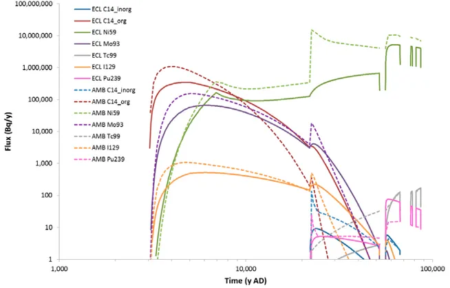
In the Global Warming Calculation Case, there is assumed to be no radionuclide release or transport during the first 1000 y. This is anticipated by SKB to be a cautious assumption as it ensures radionuclides are not released to the marine biosphere that exists from the present day to 1000 y post-closure. A variant case (the Timing of Releases Calculation Case) is used to explore radionuclide release and transport from time zero. It was found that this is not actually a cautious assumption since the doses were broadly similar to the Global Warming Calculation Case (Section 5.1.2 in TR-14-09).
There is also assumed to be no flow during four periods of permafrost, with the first period starting at 52,000 y AD. Inspection of the ECOLEGO files confirmed that there is also assumed to be no diffusion during the periods of permafrost. This is consistent with the assumption that formation of permafrost results in freezing of the repository and complete degradation of the concrete (Table 6).
Our initial review (SSM, 2016) identified that SFR3 is deeper than SFR1, so it is possible that SFR1 may be frozen during periods of permafrost while SFR3 is not (Figure 7-1 in TR-14-01). In this situation, transport by diffusion would still be possible in SFR3, but complete degradation of the concrete would not occur. Once the concrete barriers in 2BMA have become severely / completely degraded, radionuclide transport through them is calculated using a fracture flow model, rather than treating them as porous media. This is indicted by ‘F’ in Table 6. Appendix D in TR-14-09 explains that in the fracture flow model there is assumed to be no sorption of radionuclides onto fractures in the concrete. However, Section 6.6.3 in TR-14-01 states that when the permafrost melts and the concrete is completely degraded it no longer limits advective flow, but continues to act as a sorption barrier. Therefore SKB’s conceptualisation and mathematical model of this transition are unclear.
It is also not clear if this fracture flow models only applies to the construction concrete, or also the grout, concrete moulds and cementitious wasteforms. In the AMBER model, the fracture flow model has been applied to the concrete caissons and concrete moulds, but not to the grout surrounding the waste packages or the cementitious wasteforms.
The time periods for evolution of the material properties and flows are further described in the following sub-sections.
Table 6. Evolution of near-field hydrological cases (Table 4-1 in TR-14-09)
2.3.6 Material Properties
Material properties are given in Section 4.1 in TR-14-09 and are reproduced in Table 7 to Table 9. For effective diffusivity and porosity data, p41 in TR-14-09 notes that, “the transitions between time periods were modelled as a gradual change
over 100 years (but over 10 years for the first transition at 2100 AD)”. Time
invariant values are provided for densities.
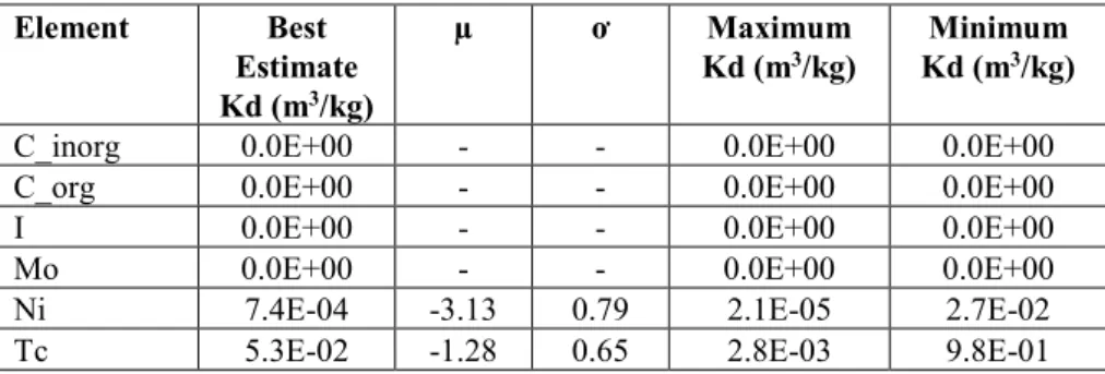
Effective diffusivities and porosities of construction concrete were specified as probability density functions (PDFs). The values are taken from Table 9-5 and Table 10-4 in 14-10. Anion exclusion factors are not specified in 14-09, TR-14-10, or TR-14-12 for cementitious materials, so we assumed this is not a relevant process.
The shape of the PDF is not specified for the porosity data range. Section 10.8 in TR-14-10 explains that insufficient data are available to describe the distributions of hydraulic parameters. Therefore, deterministic values are used in the ECOLEGO models. We note that there may be a slight discrepancy between Table 4-2 in TR-14-09 and Table 9-5 in TR-14-10 with the former describing a time period to 52,000 AD and the latter to 54,000 AD. We also note that TR-14-10 states that as far as possible the parameter values are taken from the work of Höglund (2014: R-13-40). Table 10-4 in TR-14-10 gives porosities of 0.5 for construction concrete and moulds beyond 50,000 y, but Table 9-1 in R-13-40 gives values of 0.3. So the audit trail for these long-term values is not transparent.
It is not clear if the densities are grain densities, or bulk densities (i.e. grain density multiplied by (1 – porosity)). In the AMBER model they have been assumed to be bulk densities.
Table 6. Evolution of near-field hydrological cases (Table 4-1 in TR-14-09)
2.3.6 Material Properties
Material properties are given in Section 4.1 in TR-14-09 and are reproduced in Table 7 to Table 9. For effective diffusivity and porosity data, p41 in TR-14-09 notes that, “the transitions between time periods were modelled as a gradual change
over 100 years (but over 10 years for the first transition at 2100 AD)”. Time
invariant values are provided for densities.
Effective diffusivities and porosities of construction concrete were specified as probability density functions (PDFs). The values are taken from Table 9-5 and Table 10-4 in 14-10. Anion exclusion factors are not specified in 14-09, TR-14-10, or TR-14-12 for cementitious materials, so we assumed this is not a relevant process.
The shape of the PDF is not specified for the porosity data range. Section 10.8 in TR-14-10 explains that insufficient data are available to describe the distributions of hydraulic parameters. Therefore, deterministic values are used in the ECOLEGO models. We note that there may be a slight discrepancy between Table 4-2 in TR-14-09 and Table 9-5 in TR-14-10 with the former describing a time period to 52,000 AD and the latter to 54,000 AD. We also note that TR-14-10 states that as far as possible the parameter values are taken from the work of Höglund (2014: R-13-40). Table 10-4 in TR-14-10 gives porosities of 0.5 for construction concrete and moulds beyond 50,000 y, but Table 9-1 in R-13-40 gives values of 0.3. So the audit trail for these long-term values is not transparent.
It is not clear if the densities are grain densities, or bulk densities (i.e. grain density multiplied by (1 – porosity)). In the AMBER model they have been assumed to be bulk densities.
Data have not been found in SKB’s reports for the cementitious wasteforms. Inspection of the ECOLEGO models files revealed three different materials types that might correspond to the cementitious wasteforms. These are: waste cement; waste wall concrete; and waste concrete. However, without greater familiarity of the ECOLEGO code, it was not possible to deduce how these map to the waste package compartments. In addition, some of the associated properties appear to be effective properties. The logic underpinning these effective properties is not known. The properties of the cementitious wasteforms (solidified waste and embedded waste) were set to be the same as grout in the AMBER model. Sensitivity to the properties of the wasteforms was then explored as a variant calculation case. Table 7. Effective diffusivities (De) (m2/s) (Table 4-2 in TR-14-09 and Table 9-5 in TR-14-10)
Time AD 2000 -
2100 2100 – 12,000 12,000 – 22,000 22,000 – 52,000 52,000 – 102,000
Construction
concrete De 3.50E-12 5.00E-12 5.00E-12 1.00E-11 2.00E-10
PDF N/A N/A N/A Log
triangular Min 8.0E-12 Max 2.0E-11 Log triangular Min 2.0E-11 Max 2.0E-10 Moulds De
3.50E-12 2.00E-11 5.00E-11 1.00E-10 5.00E-10
PDF N/A N/A N/A N/A N/A
Grout De
3.50E-10 4.00E-10 4.00E-10 5.00E-10 1.00E-9
PDF N/A N/A N/A N/A N/A
Macadam De 6E-10 6E-10 6E-10 6E-10 6E-10
PDF N/A N/A N/A N/A N/A
Table 8. Porosities (-) (Table 4-3 in TR-14-09 and Table 10-4 in TR-14-10)
Time AD 2000 - 2100 2100 – 12000 12000 – 22,000 22,000 – 52,000 52,000 – 102,000 Construction
concrete Porosity PDF 0.11 N/A 0.14 Range 0.14 0.18 0.5 0.11-0.16 Range 0.11-0.16 Range 0.16-0.20 N/A Moulds Porosity 0.11 0.14 0.14 0.18 0.5 PDF N/A Range 0.11-0.16 Range 0.11-0.16 Range 0.16-0.20 N/A Grout Porosity 0.3 0.4 0.4 0.5 0.5
PDF N/A N/A N/A N/A N/A
Macadam Porosity 0.3 0.3 0.3 0.3 0.3
Table 9. Densities (kg/m3) (Section 4.1 in TR-14-09)
Material Density (kg/m3) Notes
Construction concrete 2,529
Moulds 2,529 Not specified so assumed
to be the same as a construction concrete
Grout 2,250
Macadam 1,890 Rock density 2700 kg/m3
from TR-10-52. Macadam density calculated based on a porosity of 0.3.
2.3.7 Flows
Section 9.3.2 in TR-14-09 describes how, “the compartments of the RNT near-field
model coincide with control volumes of the near-field hydrological model (or sub volumes thereof). The flows from one compartment to another are determined by calculating the flow across the surfaces of the control volumes. The sub-division of control volumes into several compartments for achieving a finer resolution in the radionuclide transport applies particularly to the concrete walls of the models of the BMA vaults and the Silo. The subdivision of the concrete walls is done to avoid the large numerical dispersion that would result from representing the walls with only one compartment each. In the radionuclide transport model, all outer walls were represented by five compartments each”.
The control volumes for 2BMA are illustrated in Figure 3. They are further described in Section 3.3 in TR-13-08:
“– Each waste compartment is delimited by a concrete barrier on top, bottom, and lateral sides. These outer concrete walls define the waste control volumes. The waste control volumes are numbered from 1 in the south to 14 in the north. – There are also 14 control volumes (backfill) surrounding the waste control volumes. Note that unlike the 1BMA there are no concrete walls between the waste storage sections in this case. The limits of the backfill control volumes are chosen exactly in the middle of the two volumes (see Figure 3‑162– on the right side).
Because of this the size of backfill control volume 14 is slightly bigger.”
The same control volumes have been used to parameterise the AMBER model. However, the compartment representing the macadam surrounding caisson 14 was set to be the same size as the other caissons in AMBER, so the diffusion length to the adjacent macadam compartment is the same in either direction. This simplifies implementation of diffusion in the model as diffusive transfers in the different directions do not have to be parameterised with different diffusion lengths.
2 Figure 3 in this report.
Figure 7-7 in R-13-08 is reproduced as Figure 10. It shows the effect of the hydraulic cage provided by the engineering as built (base case), with flows through the macadam being several orders of magnitude greater than flows through the waste. The results also show an approximate order of magnitude change in flow through the wastes along the length of the vault. The different shoreline positions correspond to 2000 AD, 3000 AD and 5000 AD. The shoreline position has limited influence of the total flow through the vault.
Figure 10. Flows through the 2BMA vault with as built properties (Figure 7-7 in R-13-08) Assessment Model Flowchart (AMF) 50 in TR-14-12 describes where the water flow volumes through the different control volumes are stored for input to the radionuclide transport model. However, they are not reported. The complete flow data set was provided by SKB in three Excel spreadsheets. The spreadsheets give the flow out of each of the six sides of each control volume: x-, x+, y-, y+, z-, z+. Interrogation of the ECOLEGO model clarified that the y direction corresponds to the long axis of the vault SKB’s model.
All the data from the spreadsheets are read into the ECOLEGO model and are processed inside the model. Negative flows are set to zero, so positive flows must represent flow out of the control volume, and negative flow must represent flow in. The relevant flow is then selected in ECOLEGO depending on the shoreline position and concrete degradation state.
For the AMBER model, the flows were pre-processed in the spreadsheets prior to being entered into the model. The radial representation of the waste packages, grout and caissons, means that flows in different directions do not need to be distinguished for these compartments, so the positive flows can be summed into a single flow
volume. Flow out of the macadam can either be into the adjacent rock or adjacent macadam. Therefore, flows parallel and perpendicular to the long axis of the vault were distinguished. This is illustrated in Figure 11. The flow values used in the AMBER model are given in Table 10.
Figure 11. Representation of flows by advective transfers between compartments in AMBER Table 10. Flows (m3/y) through control volumes in the 2BMA vault pre-processed for the AMBER
model, at times corresponding to different shoreline positions (2000, 3000 and 5000 AD) and concrete degradation states (Table 6)
Time (AD)
Caisson Flow (m3/y) 2000 3000 5000 22,000 52,000
1 Macadam parallel 1.77E-01 3.85E+00 3.37E+00 3.38E+00 3.39E+00 1 Macadam perpendicular 0.00E+00 9.25E-02 6.50E-01 6.52E-01 6.54E-01 1 Caisson 3.98E-04 4.81E-03 5.56E-03 3.92E-01 1.91E+00 2 Macadam parallel 2.10E-01 6.59E+00 6.31E+00 6.31E+00 6.33E+00 2 Macadam perpendicular 0.00E+00 8.65E-02 2.50E-01 2.50E-01 2.48E-01 2 Caisson 3.24E-04 7.93E-03 8.21E-03 5.67E-01 2.91E+00 3 Macadam parallel 2.24E-01 7.61E+00 7.25E+00 7.25E+00 7.27E+00 3 Macadam perpendicular 8.18E-03 1.17E-01 1.54E-01 1.55E-01 1.53E-01 3 Caisson 2.93E-04 9.62E-03 9.65E-03 6.65E-01 3.42E+00 4 Macadam parallel 2.28E-01 8.39E+00 7.96E+00 7.96E+00 7.98E+00 4 Macadam perpendicular 1.07E-03 4.89E-02 1.76E-01 1.74E-01 1.70E-01 4 Caisson 2.93E-04 1.19E-02 1.30E-02 8.56E-01 4.15E+00 5 Macadam parallel 2.64E-01 1.46E+01 1.45E+01 1.46E+01 1.46E+01 5 Macadam perpendicular 1.38E-02 1.33E+00 2.36E+00 2.36E+00 2.36E+00 5 Caisson 4.61E-04 2.23E-02 2.71E-02 1.77E+00 7.90E+00 6 Macadam parallel 2.64E-01 1.53E+01 1.54E+01 1.54E+01 1.54E+01 6 Macadam perpendicular 2.64E-03 1.40E-01 2.52E-01 2.50E-01 2.46E-01