Wealth Inequality : Analysis based on 21 EU countries

(1)

Wealth Inequality

Analysis based on 21 EU countries

BACHELOR

THESIS WITHIN: Economics NUMBER OF CREDITS: 15 ECTs PROGRAMME OF STUDY: International Economics

AUTHOR: Mengying Man, Meixuan Ren JÖNKÖPING May 2019

(2)

(3)

Bachelor Thesis in Economics

Title: Wealth Inequality: analysis based on 21 European Union countries Authors: Mengying Man and Meixuan Ren

Tutor: Tina Wallin and Toni Duras Date: 2019-05-20

Key terms: Wealth inequality, Gini index, Housing Price Index, Minimum wage, Inflation rate

Abstract

The aim of this thesis is to examine how wealth inequality alters when macroeconomic factors such as housing price index, inflation rate, and minimum wage change. In the theoretical part, the potential connection between some macroeconomic factors and wealth inequality is described through the link of the Lorenz Curve and Pareto distribution. In the empirical part, we analyze the development of wealth inequality in 21 countries from the European Union from 2004 to 2015. The study presents significant evidence that the housing price index is negatively correlated with wealth inequality while similar conclusions cannot be made regarding inflation rate and minimum wage. In this paper, the Gini index is used as a proxy for wealth inequality.

(4)

1. Introduction

1.1 Background and Aim

In present time, the phenomenon of wealth inequality has become an increasingly serious and ubiquitous issue both on a national and international level. In 2017, the richest 1% of the world population own more than half of the world’s total wealth (Frank, 2017). Moreover, according to the annual report of Oxfam, the poorest half of the world population had no increase in wealth 2018 whereas 82% of the wealth produced went to the richest 1% of the population (Hope, 2018). As a result, the wealth inequality kept growing, in 2017, the poorest 50% of the population combined hold the same amount of wealth as the 61 richest persons in the world, and by 2018, the number was down to 42 (Hope, 2018). Meanwhile, the number of billionaires has also increased, with many of them concentrated in the U.S., Japan, Germany, and China. On a national level, according to Ventura’s research containing data of 107 countries, in 2018 over 70% of countries experienced severe inequality in wealth (Ventura, 2018). All in all, conclusive data shows that the disparity between wealth and poverty is only becoming more apparent (Shan, 2018).

Having wealth concentrated on a small amount of people has been proven as a barrier to maintain social harmony. As measured by Gini index, wealth inequality will result in more crime incidents (Fajnzylber et al., 2002). Furthermore, severe wealth inequality is claimed to have a large possibility to cause a high level of poverty, which has adverse effects on the economic growth, health, and the level of education in society (Birdsong, 2015). However, it is unrealistic to eliminate wealth inequality. This is because the inequality of wealth and income is an essential feature of the market economy (Mises, 1955).

Wealth inequality has already attracted the high attention of many sociologists and politicians. Effective regulations and government intervention are considered viable solutions to create a reasonable distribution of wealth. According to Greenlaw (2014), the level of economic inequality can be altered by policies through the redistribution between the rich and the poor. Fostering a productive and prosperous economy by reducing wealth inequality could be achieved via a variety of economic policies. What

(7)

factors affect wealth inequality? And to what extent can the government change and control it? The positive effect of taxation to alleviate income and wealth inequality is a common thought solution, as shown in Figure 1, the Gini coefficient before tax and after tax in 34 countries from all over the world in 2014.

Source: Datawrapper

Figure 1 Comparison of Gini coefficients after tax and before tax in 2014

According to the figure, the blue line representing the after-tax Gini coefficients is always below the red line which represents the pre-tax figures, which indicates a positive taxation effect on alleviating income and wealth inequality. This thesis aims to find out other potential factors that may affect income and wealth inequality, so as to provide policy recommendations for the government.

1.2 Research Question

The research question that is going to be answered in this thesis is whether wealth

inequality increases or decreases when the macroeconomic factors, the housing price index, the minimum wage, and the inflation rate change. In order to answer this

question, the following sections will analyze several explanatory variables and how they influence wealth concentration. Moreover, the empirical analysis will help explain our research question by examining the Gini coefficient of different countries. This

0 0.1 0.2 0.3 0.4 0.5 0.6 Ice la n d Sl ova k R epu bli c Sl ovenia De n m ar k C ze ch R epu bli c Fi n la n d N or w ay Be lgi u m A u str ia Sw ede n Luxe mbou rg Hu n ga ry G er ma n y Fra n ce Sw it ze rla n d Ir el an d P ola n d K or ea N ethe rla n ds C an ada _Italy A u str ali a P or tugal G re ece Spa in Es tonia N ew Z ea la n d La tvi a Un it ed K in gdom Israel Li th u an ia Un it ed Sta te s Tu rk ey Me xico

Comparison of Gini Coefficient after tax and before tax in 2014

(8)

Bulgaria, Croatia, Czech Republic, Estonia, France, Greece, Hungary, Ireland, Latvia, Lithuania, Luxembourg, Malta, Netherlands, Poland, Portugal, Romania, Slovak Republic, Slovenia, Spain, and United Kingdom. Besides, the study utilizes data mostly between 2004 and 2015.

As mentioned previously, the study aims to analyze the effect of macro factors on wealth inequality. Among all economic factors, three will be closely examined: housing price index (HPI), minimum wage, and inflation rate. Furthermore, the wealth inequality is to be presented by the Gini coefficient or Gini index, which is a common measure of wealth inequality (Tobochnik, Christian & Gould, n.d). Changes in the Gini Coefficient might provide insight on the development of wealth inequality.

1.3 Delimitation

Data is the most significant limitation in our study. The selection of both countries and time period is greatly restrained. We tried to find the available data of four variables including housing price index, minimum wage, inflation rate and Gini index of all countries of EU. However, some data is missing in terms of the cross-sectional and the time period aspect. To deal with it, the unbalanced panel data model can be a solution, which will be explained in detail in the following parts. However, the data of the Gini index used as the dependent variable in our panel data model can only measure the relative wealth inequality because it is pretty difficult to find the Gini index of measuring absolute wealth inequality. There are two reasons making it so hard to get the Gini index of absolute wealth inequality. Firstly, the value of assets is much harder to access than annual income. Secondly, wealthier households tend to under-report their total wealth for tax-related purposes (Fuller et.al, 2019). However, researchers can use the Gini index from the world bank to measure relative wealth distribution of a country.

In this study, data of 21 countries in European Union is collected as our observations, which may have correlation among cross-sectional data since they are all member states of the European Union (Economy Watch, 2010). Therefore, the correlation between the macroeconomic factors by using panel data analysis cannot be eliminated completely.

(9)

In addition, this thesis will not study the magnitude relationship between the dependent variables and independent variables but investigate if the independent variables significantly affect the dependent variable and study the direction of their impact on the Gini index. Furthermore, it is impossible for us to investigate all of the potential influencing factors of wealth inequality in this thesis. Therefore, three potential influencing factors (Housing Price Index, minimum wage, inflation rate) are going to be focused on, and their effect on wealth inequality in different countries among the EU will be analyzed.

1.4 Structure

Section 2 presents a theoretical framework regarding the Lorenz Curve and Pareto distribution will be presented to support the following discussion and analysis. Then, the literature review in terms of the possible impact of three macroeconomic factors on the wealth inequality will be stated in Section 3. In section 4, the expected signs that the independent variables could have are briefly discussed. And section 5 will explain the data collected to make this analysis and there will be a specific introduction of three macroeconomic factors and their calculations. Section 6 will describe the panel data model and the LSDV method in detail, and in section 7, the regression results and corresponding analysis for every independent variable will be presented, and the possible reasons behind the impact they show on the dependent variable, Gini index, are to be discussed. Section 8 will summarize the whole thesis, draw the conclusion and propose some recommendations for controlling wealth inequality in the EU, also put forward meaningful further study in this topic.

2. Theoretical Framework

In this section, to answer the research question, Lorenz curve, Gini index, Pareto distribution and the connections between them will be introduced, which are used to present the theoretical framework. And an explanation of how wealth inequality will alter due to the change of Pareto shape parameter is given. When the shape parameter increases, wealth inequality will diminish, vice versa.

(10)

2.1 Lorenz Curve and Gini Coefficient

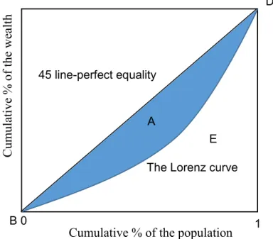
To measure the wealth inequality of a country, the Lorenz curve is considered as the graphical representations of the distribution of wealth. It plots the cumulative percentage of wealth to the percentage of the population which are in the vertical axis and horizontal axis respectively in the graph below (Kakwani & Podder, 2008). As Figure 2 shows, the whole graph is split by a 45-line that represents perfect equality between the cumulative percentage of wealth and the percentage of the population.

𝐺𝑖𝑛𝑖 𝑐𝑜𝑒𝑓𝑓𝑖𝑐𝑖𝑒𝑛𝑡 =𝑡ℎ𝑒 𝑠ℎ𝑎𝑑𝑒𝑑 𝑎𝑟𝑒𝑎 𝐴 𝐴 + 𝐸

When unequal wealth distribution exists, the Lorenz curve is bowed out. The greater the wealth inequality, the more that the line bowed further from the diagonal, vice versa. This curve starts at the origin (0,0) and ends at the point (1,1). Since A+E=0.5, the equation of Gini coefficient can be rearranged. In this way, Gini coefficient=1-2E.

Cumulative % of the population 100%

B 0

D

A

The Lorenz curve 45 line-perfect equality

Figure 2 Lorenz Curve and Gini Coefficient

E 1 C umul ati ve % of the we alt h

(11)

The Gini coefficient is a numerical measure of the extent of inequality, as the equation shows, the coefficient is the ratio that the area between the Lorenz curve and the perfect equality line is divided by the area that is under the diagonal (Tobochnik, Christian & Gould, n.d). As wealth distribution becomes more unequal, the Lorenz curve will be bowed out further, and the area of A will be larger. Therefore, the bigger the Gini coefficient, the more unequal of a country’s wealth distribution. If the Gini coefficient equals 0, wealth is perfectly equally distributed. If the Gini coefficient equals 1, the whole wealth is owned by single individual, which is a situation of perfect inequality. However, neither perfect equality nor perfect inequality, the two extremes, will exist when considering the wealth distribution of a country in reality. As such, the Gini coefficient is supposed to take values between 0 and 1.

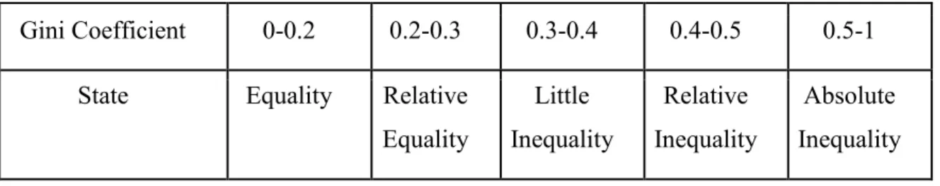
Table 1 Gini Coefficient and the inequality

Source: United Nations

2.2 Pareto Distribution

The Pareto distribution proposed by Vilfredo Pareto in 1896 is comprehensively used in the fields of sociology, actuarial science and so on, which can be applied to describe some observable phenomena by a power-law probability distribution. The power law is a functional relationship between two quantities when one quantity relatively changes, a proportional relative change would occur in another quantity. It emphasizes that one quantity is varied with the power of another quantity, independent of the initial sizes of these quantities. For Type 1 Pareto distribution, it is characterized by a scale parameter 𝑥_𝑚 and a shape parameter 𝛼 (which also can be called “Pareto index” when this distribution is used to model the distribution of wealth). It indicates that for a random variable X, the probability that X is larger than some number x is given by:

Gini Coefficient 0-0.2 0.2-0.3 0.3-0.4 0.4-0.5 0.5-1

State Equality Relative

Equality Little Inequality Relative Inequality Absolute Inequality

(12)

𝐹̅(x) = Pr(X > x) = {( 𝑋𝑚 𝑥) 𝛼 , x ≥ 𝑥_𝑚 1 , 𝑥 < 𝑥_𝑚 where 𝑥_𝑚 is the minimum possible value of X.

According to the definition, the cumulative distribution function (CDF) of a random variable with parameter 𝑥_𝑚 and 𝛼 is shown as:

𝐹𝑋(x) = { 1 − (𝑥𝑚 𝑥) 𝛼_{, 𝑥 ≥ 𝑥} 𝑚 0 , 𝑥 < 𝑥𝑚

By applying Pareto distribution to the allocation of wealth, Pareto (1896) found the "80-20 rule", also known as the Pareto principle. The rule describes the wealth allocation as an exponential model, where 20% of the population receive 80% of the wealth, and 20% of the richest receive 80% of that 80% and so on. This principle also can be derived from the Lorenz Curve. In the following part, how the Lorenz Curve is connected with Pareto distribution is displayed.

2.3 Lorenz Curve and Pareto Distribution

Given any distribution function F(x), the Lorenz curve in terms of CDF can be written as Pr(X≤ 𝑥) 𝛼 = 1 𝛼 = 2 𝛼 = 3 𝛼 = ∞ x

(13)

L(F) = ∫ 𝑥(𝐹′)𝑑𝐹′

𝐹 0

∫ 𝑥(𝐹1 ′)𝑑𝐹′ 0

where X(F) is the inverse of CDF.

And for Pareto distribution, X(F) can be expressed as x(F) = 𝑥𝑚

(1−𝐹)

1 𝛼

Considering the Pareto distribution, the Lorenz curve can be written in terms of CDF as,

𝐿(𝐹) = 1 − (1 − 𝐹)1−𝛼1, 0< 𝛼 < 1

Then, reconsider the function of the Gini index by plugging in the new expression, it can be given as:

G = 1-2∫ (1 − (1 − 𝐹)1 1−𝛼1) 𝑑𝐹

0 =

1

2𝛼−1, for 𝛼 ≥ 1

In this way, a negative relationship is built directly between the Pareto index 𝛼 and the Gini index. When 𝛼 increases (decrease), the Gini index will decrease (increase) accordingly, thus, the inequality of income or wealth will decrease (increase).

Some studies show that the shape parameter 𝛼 can be adjusted by macroeconomic factors. Piketty (2014) first proposed that the gap between real interest rate r and the growth rate of income per capita g was able to affect the shape parameter of Pareto distribution. In 2015, Piketty and Zucman claimed that wealth inequality was an increasing function with (1+r)/(1+g) in a steady state. Then, a function to illustrate this influence relationship between r, g and 𝛼 were worked out by Acemoglu (2015) in the same year.

𝛼 = 1-ln (1+

1+𝑟−𝛽 1+𝑔 )

𝜎2_/2

where 𝛽 is the marginal propensity to consume out of wealth (which is assumed to be zero in Piketty’s research) and 𝜎2_{is the variance of Pareto distribution.}

(14)

As stated in the formula, there is a clear relationship between macroeconomic factors r, g and the shape parameter 𝛼 of Pareto distribution. Therefore, the crucial link between specific economic data and theory can be established by Pareto Distribution, which can indicate how macroeconomic factors affect wealth inequality from a theoretical perspective (Jones, 2015). Once some macroeconomic factors fluctuate, the shape parameter of Pareto distribution will adjust correspondingly, thereby resulting in a shifted Lorenz Curve, eventually, the impact on the degree of wealth inequality can be observed by a changed Gini index.

As Bloomenthal (2019) held, macroeconomic factors are influential fiscal, natural or geopolitical events which have the ability to extensively affect a regional or national economy. In line with this definition, it is to be expected that housing price, minimum wage and inflation rate which can broadly affect the households’ behavior and the economic environment of a region may have similar effects as r and g on the wealth inequality.

3. Literature Review

3.1 Housing price and wealth inequality

As an important component of people's wealth, housing is considered by a number of economists to be related to the degree of wealth inequality. Bastagli and Hills (2012) realized that the fluctuation of housing price can play a dominant role in wealth

Figure 4 Theoretical Framework

Shape parameter of the Pareto distribution Housing price index Minimum wage Macroeconomic Factor Inflation rate Gini Coefficient

(15)

inequality. They removed the effect of real increase in housing price and then examined the impact of remaining part on wealth distribution over the period from 1995 to 2005 in the panel database of the United Kingdom. It was found that the decrease in wealth inequality is largely driven by an increase in housing price, rather than home ownership change and repayment of mortgages. This view was further strengthened in a recent study of housing prices and wealth inequality in Western Europe countries by Fuller, Johnston, and Regan (2019). Additionally, Bastagli and Hills (2012) also claimed a negative relationship between housing price and the degree of wealth inequality indicating that wealth tended to be more overall equally with a rising housing price. They attributed this phenomenon to the adjustment effect causing by the wealth of “the middle class”. With an increasing housing price, the total net worth of the middle class household experienced a dramatic increase compared with the top wealth households, due to the fact that housing accounts for a large proportion of wealth portfolio for the middle class.

However, other researchers put forward different ideas in other papers. For instance, Fuller (2019) held that a rising housing price had the potential to increase the degree of wealth inequality. They set up a series of Error Correction Models using data based on 13 countries to show that housing price inflation has a positive and significant effect on the wealth-to-income ratio both in the long run and short run (more considerable in short run), thereby housing price inflation will affect wealth distribution among households. Then, they also held that housing price inflation could result in a higher degree of wealth inequality due to the fact that it exacerbated cleavages between the older and younger generation. Besides, Chen and Qiu (2011) also found the deterioration effect of the uneven distribution of wealth in their Bewley model considering China as the research object. In their paper, they proposed that an inflated housing price could stimulate the investment needs of real estate for wealthy people, which further pushed up the price of houses. As a result, the wealth of the middle class and the poor were compressed, and the possibilities of purchasing a house for the poor went down, resulting in more abnormal wealth distribution.

(16)

(1996) thought that the housing price would have an uncertain effect on the degree of wealth inequality, which depends on local housing allocations. For those regions where the affluent households had already possessed plenty of initial housing equity at the start of the boom and as the main beneficiary of inflated housing price gained wealth, the regional wealth gap would widen between the rich and the poor. Otherwise, if the larger proportion of housing was owned by the low-income households, the region would have a high possibility to experience a more equal wealth distribution with a growing housing price.

3.2 Minimum wage and wealth inequality

Freeman presented the redistribution theory in 1996, which discussed how the minimum wage accomplishes to redistribute the earnings to low-paid workers. There was a debate about the efficiency of the minimum wage. Adams and Neumark (2005) thought that employment losses may occur from the minimum wage because the minimum wage had the possibility to reduce the share of low-paid employment. While study from Card and Krueger (1995) presented that employment did not decrease; with a study showing employment increased after the minimum wage was raised. To answer how the minimum wage shifted earnings, three potential groups of payers were discussed by Freeman. The minimum wage shifted earnings to the low-paid workers, some groups were supposed to pay for it, which depended on the labor market and the social welfare the country proposed.

The first group was the customers of the products of minimum wage employees. The minimum wage would increase the cost of production on goods and services which were produced by the low-paid workers. As a result, the price of these goods and services would be higher than before, which in turn decreased the purchasing power of other people who bought these goods and services. No matter who paid for it, the degree of inequality would be altered. Companies that hire low-paid workers were the second group who paid for a minimum wage. As businesses need to raise the wage for some workers, to some extent, the cost of hiring a worker was higher. And then the profit that the company could make would decline. Hence, the income that stakeholders could receive will be lower, while the low-paid workers got a higher salary, which influenced the equality. The last group for minimum wage affecting the redistribution of income

(17)

was the group of people who lost their jobs because of the set of the minimum wage. Adam Smith held the idea that supply would equal demand in a competitive market. But when a minimum wage is imposed, this equilibrium will be broken since the supply will not equal to demand any more. In other words, excess supply happens so that unemployment is created.

Some proportion of the low-paid workers could get a higher wage at the expense of another group of workers. Under this circumstance, the imposition of the minimum wage would reduce the wages of low-paid workers due to unemployment. Consequently, inequality would be larger. However, a debate exists on whether the imposition of minimum wage can create employment. A study shows that minimum wage does not increase unemployment while other well-structures researches find that employment increases after the increase of the minimum wage (Card & Krueger, 1995).

Something worth noting is that the implementation of the minimum wage is not available in some countries, such as Austria, Denmark and Sweden and so on. In these countries, there is no official law to implement the minimum wage due to their social structure, which accounts for unavailable minimum wage for these countries. Other effective wage systems exist to balance employers and employees. For example, minimum wages in Sweden are not implemented by law but are bargained by employers and trade unions and form labour agreements (Skedinger, 2010).

3.3 Inflation rate and wealth inequality

Inflation attracted a large number of researchers to investigate whether it can affect wealth inequality or not and their correlation direction. Budd and Seiders (1971) studied the impact of inflation on the degree of wealth inequality of the United States from the post-World War II period. They claimed that inflation could lead to a small but fairly consistent shift to less inequality in terms of wealth net worth. Since the shares of quantiles below the 80th_{percentile increased, the very top class lost a little wealth}

relatively. Wolff (1979) also observed an alleviating effect which an increasing inflation rate caused on wealth inequality. He focused on the impact of inflation on

(18)

was found that the poor gained more than the rich due to inflation in a simulation model, which alleviated the concentrated wealth distribution.

By contrast, Heer and Süssmuth (2003) proved a significant and positive relationship between inflation and wealth inequality by establishing a general equilibrium OLG model based on the characteristics of the US economy. They found that an increasing inflation from 5% to 20% could result in a decreasing aggregate wealth, and brought a more unequal distribution of wealth and capital at the same time. In 1974, Bach and Stephenson emphasized that unanticipated inflation could promote wealth redistribution by transferring purchasing power from the old to the young, from the very wealthy and very poor people to the middle class. In 2007, Heer and Süssmuth continued their study and investigated the relationship between anticipated inflation and wealth inequality to supplement the study of Bach and Stephenson (1974) by the general equilibrium OLG model again. Compared the different influences of a high-inflation regime (with an high-inflation rate of 6.43% annually) and a low-high-inflation regime (with an inflation rate of 3.06% annually) on the distribution of wealth, they found that higher anticipated inflation rate increased wealth inequality significantly. They regarded this result as one of the consequences of the taxation on nominal interest income.

Nevertheless, the significant effect of inflation rate does not always appear while taking other countries and period as consideration. As presented in the working paper from IMF, Ho and Ho (2016) set up a dynamic general equilibrium model based on Chinese data between 1995 and 2002 and made a counterfactual experiment to test the impact of inflation on wealth inequality. They replaced the inflation rate in 1995 by that in 2002 and kept other parameter values constant then draw the Lorenz curve for both situations. They observed that two Lorenz curves were basically coincident. And the Gini coefficient for wealth distribution also changed very slightly. Therefore, they came to the conclusion that inflation rate did not affect the degree of wealth distribution significantly.

(19)

4. Expected Result

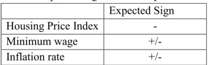
Table 2 Expected Sign of the independent variables Expected Sign

Housing Price Index -

Minimum wage +/-

Inflation rate +/-

In the beginning, we expected significant relationships could exist between three independent variables and the dependent variables. However, we have different expectations regarding the signs of the impact that these independent variables could have on the extent of wealth inequality.

In Europe, “the middle class” first appeared in the late middle ages, then experienced dramatic expansion in the 19th century as a result of the Industrial Revolution (Jones, 1997). This term describes a social group in the middle of the social hierarchy, usually has an income range to define them in a given society (Amadeo, 2019). Households in the middle class can support their life and most of them own residences. Europe has been considered as the typical middle-class society historically, with the lower levels of inequality and the comprehensive welfare state (Bussolo et. al, 2018). Although in recent years, some economists (such as Vaughan-Whitehead, 2016) have questioned about the decline of the middle class in Europe, it still occupies a considerable proportion in the economic system of European societies and plays a vital role regarding the change of wealth distribution. Hence, we expect a negative relationship between them, meaning that the degree of wealth inequality has a high possibility to be lower with a rising housing price in EU. Because when housing price increases, the middle class as the large proportion of population in the society will have a higher total wealth value. And the middle class who consider the housing as their main wealth will gain more than the top class, leading to a downward trend of wealth concentration.

In line with the literatures and the report from European Commission in 2018, minimum wage appears to have some negative effect on the employment of the low-paid groups, which correspond to the redistribution theory presented by Freeman in 1996. The effect that the minimum wage could have on wealth inequality depends on the unemployment

(20)

condition caused by the minimum wage. Therefore, we expect that the implementation of minimum wage could have a positive or negative sign on the wealth inequality.

Lastly, we expect that the inflation rate can have a significant effect on the extent of wealth inequality in EU, but cannot infer whether it is positive or negative. According to the literature review, the anticipated inflation and unanticipated inflation has the opposite effect on wealth inequality. However, we cannot know the type of inflation between 2004 and 2015 in EU since a finance crisis swept the world from 2007 to 2009, greatly affecting the economic environment in Europe. Under this circumstance, we only expect the significance of inflation rate but have a neutral attitude towards its sign.

5. Data and Variables

This section describes the collection of data and the variables used for analyzing the change in wealth inequality. The dependent variable in this study is the Gini index that represents wealth inequality, followed by a presentation of variables selection in section 5.2.

5.1 Data

In this study, the Gini index and the inflation rate are collected from the World Bank Group (WBG), and Eurostat helps with the minimum wage and housing price index. The WBG draws on a survey across 164 countries in six regions and 25 other high-income countries, which allows us to have an overview of the world condition. Gini index recorded in WBG is from 2003 to 2015, which makes it harder to collect data. Moreover, among all the countries that WBG surveyed, only 41countries in the world have the Gini index for more than 7 years. Other countries only have two or three years’ Gini index on record. To investigate the wealth inequality in the European Union, we collect 27 countries’ Gini index excluding Germany due to the lack of data. Owing to the social structure, 6 countries: Austria, Cyprus, Denmark, Finland, Italy, and Sweden does not have the official law to implement the minimum wage. As a result, only 21 EU countries’ data can be in use. Moreover, it is possible for Gini index from WBG to rise while people living in absolute poverty decreases, because the Gini index measures relative wealth instead of absolute wealth.

(21)

As mentioned previously, we collect 21 countries’ Gini index of European Union from 2004 to 2015. But for some time period, the Gini index of several countries is missing (2004 in EE and PL, 2004 and 2005 in SK, MT and BG, 2004-2006 in HU, 2004-2008 in HR, 2004-2007 in RO), which is supposed to account for the unbalanced panel data analysis. The inflation rate is also collected from the WBG. Another two explanatory variables, minimum wage and the housing price index (HPI), are collected from the Eurostat from 2004 to 2015. Eurostat provides a percentage change of residential housing compared to a specific year-2015, which is considered as the base year to calculate HPI by Eurostat.

5.2 Variables 5.2.1 Gini index

Gini index is the dependent variable in this study, as described in section 2, it measures the area between the Lorenz curve and the hypothetical line of absolute equality, expressed as a percentage of the maximum area under the line.

Gini index = Gini coefficient*100

5.2.2 Housing Price Index

Currently, housing is the most important asset of households, which is a satisfactory need for individuals and families (Karamujic, 2015). Purchasing a house is considered both as a kind of consumption and as an investment. Thus, the value of housing plays a significant role in the distribution of wealth. To measure the effect of house price on wealth distribution, the housing deflated price index is selected to give an overview of the changes on house prices in different areas. Housing deflated price index is the ratio between the house price index and the national accounts deflator for private final consumption expenditure, which indicates the inflation in house market relative to the inflation in the real consumption expenditure of households. Only market price is considered while self-build houses are excluded.

𝐻𝑃𝐼(𝑑𝑒𝑓𝑙𝑎𝑡𝑒𝑑) = Housing price index

(22)

5.2.3 Minimum Wage

Minimum wage is the lowest salary that employees can legally receive in a given period by law. Litwin (2015) used data from OECD countries to see the relationship between inequality and minimum wage. In this study, monthly national minimum wage in euros is used. This number is the amount of wage that all workers in a country or at least the majority of workers can get in a month for their work. The minimum wage in the non-Euro region is converted to euro according to the exchange rate.

5.2.4 Inflation Rate

An inflation rate that is an increasing percentage change in the price level over time plays a crucial role (Akinsola & Odhiambo, 2017). Akinsola and Odhiambo (2017) found that the impact of inflation on the economy can vary from country to country, which depends on the country-specific characteristics. By using the annual inflation rate (consumer price) as one of the explanatory variables, the distribution of wealth will become more unequal. This data reflects the annual percentage change in the cost of purchasing a basket of goods and services to the average consumer, which may be fixed or changed at specified intervals, which can be calculated by the following formula.

𝐼𝑛𝑓𝑙𝑎𝑡𝑖𝑜𝑛 𝑟𝑎𝑡𝑒 =(𝐶𝑃𝐼𝑥+1−𝐶𝑃𝐼𝑥)

𝐶𝑃𝐼𝑥 ,

Where the initial consumer price index is 𝐶𝑃𝐼𝑥, and 𝐶𝑃𝐼𝑥+1 is the changed consumer

price index.

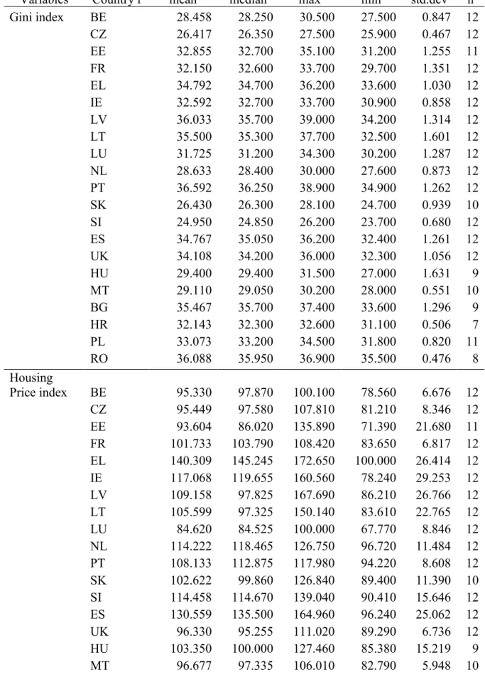
5.3 Descriptive Statistic

This regression has 231 observations from 21 European Union countries, according to the descriptive statistic in Table 3 (see Appendix 1), the mean of the Gini index among the 21 countries has a range between 24.950 and 36.592. And the standard deviation of Gini index is between 0.467 and 1.631. In terms of the small variation on Gini index, wealth accumulation may account for this. Ameriks, Caplin and Leahy (2003) proposed that long time period is needed to see the changes on households’ wealth. Table 3 also

(23)

displays the average value and standard deviation of the independent variables for each country.

6. Method

6.1 The Panel Data Model

When a phenomenon cannot be explained very comprehensively by only a cross-sectional data or only a time series, researchers can use the panel data model instead of the simple linear regression model. The panel data model allows researchers to combine the cross-sectional data and time series data to study a two-dimensional data panel, then do better work than simple linear regression in explaining dynamic change by repeating the time series data in different sections (Gujarati & Porter, 2009). Here, one of the panel data models is chosen to make the regression analysis since the variation of different countries and time period are taken into account. Specifically, the unbalanced panel data is used to make the regression due to the missing values of variables of some countries. For estimation, there are four possible methods generally: pooled OLS method, least square dummy variables (LSDV) method, fixed effect within group method and random effect method. Among them, the LSDV method is chosen.

6.2 Least Square Dummy Variables Model

LSDV estimator is pooled OLS including a set of N-1 dummy variables which identify individuals and has additional N-1 dummy variables. When using dummy variables in the regression, only N-1 dummy variables can be introduced to avoid the dummy variable trap (the situation of perfect collinearity). Unlike the random effect model, the individual-specific effect is considered here. In the LSDV method, there is a subject-specific characteristic to be the base of the intercept, which can be expressed by dummy variables. In general, it has the following formula:

𝑌𝑖𝑡 = 𝛽0+ 𝛼2𝐷2𝑖𝑡+ 𝛼3𝐷3𝑖𝑡+ ⋯ + 𝛼𝑁𝐷𝑁𝑖𝑡+ 𝛽1𝑋1𝑖𝑡+ 𝛽2𝑋2𝑖𝑡+ ⋯ + 𝛽𝑝𝑋𝑝𝑖𝑡+ 𝜀𝑖𝑡

(24)

By adding subject specific dummy variables, intercepts of the subjects may be different. The difference can be caused by the features of each subject, such as different policies issued in each country in their history. Here, “fixed effects” are due to the time-invariant intercept. In other words, although the intercept may vary across each subject, each session’s intercept does not change over time (Gujarati & Porter, 2009). In this study, 21 countries have different conditions in their government policy as well as the economic conditions, which makes it difficult to measure these effects. Thus, LSDV model can help us to fix these unknown conditions in the intercepts (reference country Belgium). The following equation is used in the study to analyze the effect the three macroeconomic factors may have on the Gini index.

Gini index = 𝛽0+ 𝛽1𝐻𝑃𝐼𝑖𝑡+ 𝛽2𝑀𝑖𝑛𝑖𝑚𝑢𝑚 𝑤𝑎𝑔𝑒𝑖𝑡+ 𝛽3𝐼𝑛𝑓𝑙𝑎𝑡𝑖𝑜𝑛 𝑟𝑎𝑡𝑒𝑖𝑡+ 𝛼1𝐷𝑐𝑧 + 𝛼₂𝐷_𝐸𝐸+ 𝛼₃𝐷_𝐹𝑅+ 𝛼₄𝐷_𝐸𝐿 + 𝛼₅𝐷_𝐼𝐸 + 𝛼₆𝐷_𝐿𝑉+ 𝛼₇𝐷_𝐿𝑇+ 𝛼₈𝐷_𝐿𝑈 + 𝛼₉𝐷_𝑁𝐿+ 𝛼₁₀𝐷_𝑃𝑇+ 𝛼₁₁𝐷_𝑆𝐾+ 𝛼₁₂𝐷_𝑆𝐼 + 𝛼₁₃𝐷_𝐸𝑆 + 𝛼₁₄𝐷_𝑈𝐾 + 𝛼₁₅𝐷_𝐻𝑈+ 𝛼₁₆𝐷_𝑀𝑇+ 𝛼₁₇𝐷_𝐵𝐺+ 𝛼₁₈𝐷_𝐻𝑅+ 𝛼19𝐷𝑃𝐿+ 𝛼20𝐷𝑅𝑂 + 𝜀𝑖𝑡

7. Model Analysis

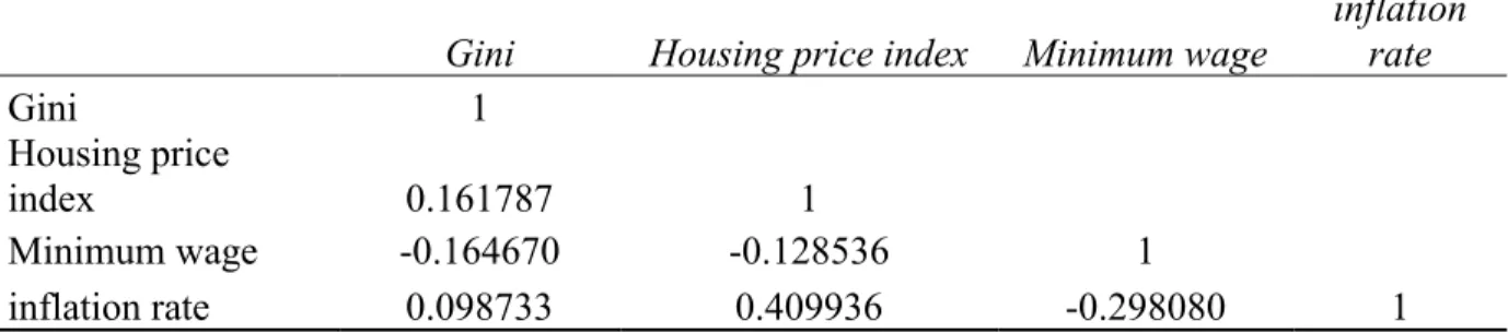
7.1 Correlation Matrix

The correlation matrix is a table showing correlation coefficients between variables, which is used to see the relations between every two variables. As shown by the Table

4, there is an overall low level of correlations between the variables. However, there is

one value that needs notice-0.409936 which represents the correlation between the inflation rate and the housing price index, but it is not high enough to concern when making the analysis (Gujarati & Porter, 2009).

Table 4 Correlation Matrix

Gini Housing price index Minimum wage

inflation rate Gini 1 Housing price index 0.161787 1 Minimum wage -0.164670 -0.128536 1 inflation rate 0.098733 0.409936 -0.298080 1

(25)

Here is the result of the unbalanced panel data model regression by EViews.

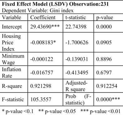
Table 5 LSDV

Fixed Effect Model (LSDV) Observation:231 Dependent Variable: Gini index

Variable Coefficient t-statistic p-value Intercept 29.43690*** 22.74398 0.0000 Housing Price Index -0.008183* -1.700626 0.0905 Minimum Wage -0.000122 -0.139031 0.8896 Inflation Rate -0.016757 -0.413495 0.6797 R-square 0.921298 Adjusted-_{R square} 0.912254 F-statistic 105.3557 Prob (F-

statistic) 0.0000*** * p-value <0.1 ** p-value <0.05 *** p-value <0.01

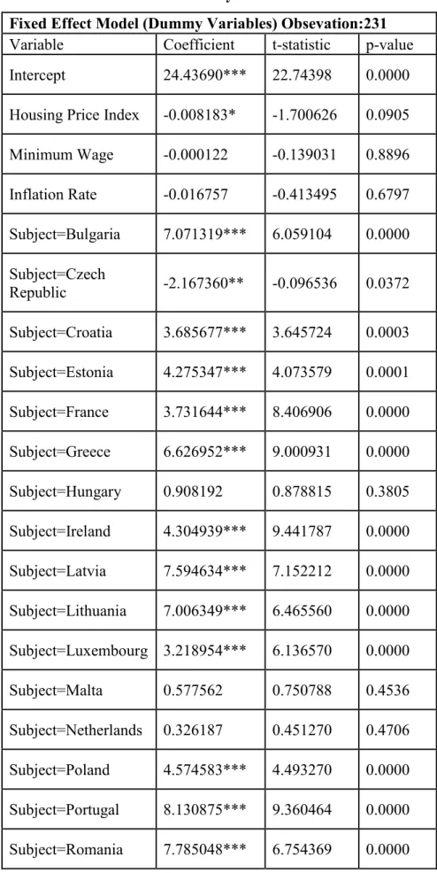
For our unbalanced panel data model, the subject “Belgium” is treated as the reference category and twenty cross-sectional dummy variables were added into the equation to distinguish the fixed effect of different countries among EU. However, there is no period dummy variable, which is not suitable for our purpose of the regression since we want to analyze the development of every country’s wealth inequality in a time period. As a result, this regression has twenty-four independent variables in total. Before starting the tests of significance, we would like to choose 0.1 as our significant level.

7.2 Test of Significance

Before we start to test the significance in the panel data model, we made unit root tests to check the stationarity of the data. All of the unit root tests for the dependent variable and independent variables show significant p-values to reject the null hypothesis, indicating a stationary dataset in the regression (see Appendix 3). According to Table

(26)

countries. We can also see that the R square has such a high value of 0.921298 causing by too many dummy variables in the regression.

Then, it comes to the analysis of every independent variable.The explanatory variable, housing price index, has a p-value which is smaller than the significant level (0.0905). Therefore, we have 90% confidence to claim that the housing price index can significantly influence the Gini index of our target countries and reveal a negative relationship between them. The estimated coefficient equal to -0.008183, indicating that there is 0.008183 decrease of Gini index with a unit increase of housing price index. It means that, for example, there is 20 units increase of price percentage (HPI shifts from 100 to 120) compared with the figure in 2015, then the Gini index average decreases of 0.16366. And we worked out that the average of the absolute value of annual variation regarding the Gini index among 21 countries is equal to 0.693928. There is no dramatic difference in the magnitude between 0.16366 and 0.693928. Hence, the change in housing price does have an important impact on the level of wealth inequality. However, it is good to mention that the value of the estimated coefficient of the housing price index is going to vary with the different reference year (2015) that is chosen. What will not change is the sign of the relationship between housing price and the degree of wealth inequality in the European Union. It will always be negative in the same model.

Investigating the reason why this result shows in our model, the research of Bastagli and Hills shed light on it. As we mentioned previously, they claimed that the negative relationship between housing price and the degree of wealth inequality could be attributed to the consequence of a large proportion of “the middle class”. The adjustment effect of the middle class allows them to gain more than the wealthy from a rising housing price. Then, a decreasing degree of wealth inequality is resulted. Therefore, the effect of a large proportion of the middle class in European Union can be treated as the reason why the housing price index shows a significant and negative relationship with the Gini index in our unbalanced panel data regression, which is also line with our expectation.

Then, it can be seen that the p-value of the coefficient of minimum wage is much larger than the significant level (0.8896), so we claim that the minimum wage cannot significantly affect the degree of wealth inequality based on twenty-one countries' data.

(27)

Having a look at the data collected from Eurostat, for some countries, the set of a minimum wage is constant over the years. To be specific, the minimum wage that some countries set do not change during some time periods. For example, in Ireland, the minimum wage is set in the level of 1461.85 euros per month from 2008 to 2015. And in Lithuania, the minimum wage is set as 231.7 euros per month from 2008 to 2012. However, Gini index changes when minimum wage keeps constant in these years since other factors having an impact on wealth inequality vary. Under this circumstance, the reason that discussed above may account for the insignificant result gotten from the regression.

For the inflation rate, according to the regression result, there is an insignificant relationship between inflation rate and Gini index in our panel data model since the p-value of is larger than the significant level (0.6797). Thinking about the reason why inflation shows an insignificant relation with wealth inequality here, the time lag of the effect of inflation is supposed to be taken into account. The impact of inflation on wealth redistribution is not only through the direct influence on people’s purchasing power, but also through affecting consumers’ future behavior and decision indirectly by changing their inflation expectation (Duca et al, 2016). However, it usually takes some time to change people’s expected inflation rate and their behavior (Bianco, 2014). Therefore, we deduce that inflation has a delayed effect on the level of wealth inequality. It is hard to see a significant change in wealth distribution in terms of fluctuating inflation rate in the 12-year time period (from 2004 to 2015). To study the relation between them, a longer time period and more observations are necessary. Also, we cannot introduce the lagged inflation rate into the regression. If we want to add it, the monthly inflation rate or weekly inflation rate are needed since the inflation rate has a high possibility to delay by several months or weeks rather than years.

From what described above, the housing price index has a relationship with the Gini index. We can summarize that to some extent, 21 countries used in this study have some common characteristics as the housing price heavily influences everyday life. And we cannot easily say that the other two variables have no effect on wealth inequality, measured by the Gini index. As a result of the limitation of data and research capability,

(28)

8. Conclusion

This thesis aims to identify macroeconomic factors which can affect the extent of wealth inequality of the countries in the European Union, a theoretical and an empirical approach are applied. In the theoretical part, the connections between the three factors and the distribution of wealth are presented. For the empirical part, LSDV model is used as a useful tool to deal with the data.

We expected that the three variables could have a significant impact on the wealth distribution at the beginning, but by analyzing unbalanced data model from the 21 countries in EU from 2004 to 2015, housing price index is the only variable with a significant correlation with wealth inequality. In terms of the reasons behind these relationships, we infer the reasons according to the literature review. Specifically, the significant effect of HPI is attributed to the influence of the middle class in Europe. For the insignificant relationship between inflation rate and Gini index, it is possibly associated with the time lag of the change of inflation expectation. Resulting from the unchanged minimum wage in some countries for several years, the variation does not exist to examine the effect that minimum wage may bring on the wealth inequality, thus, insignificant relationship is shown in the regression.

By analyzing the 21 EU countries, we cannot give a specific suggestion for the policy makers to have a great control of wealth inequality, this is because that a common policy regarding the housing price index is difficult to issue in all the countries. However, this regression result indicates that politicians possibly can try to affect wealth inequality by controlling housing price of a region. To give specific policy recommendations, a magnitude level of analysis may be in need to have a better understanding of the impact that housing price index can bring on the wealth inequality.

For further study, the Gini index for absolute wealth inequality is necessary to make a more reliable regression. Moreover, further studies containing larger sample are suggested to have a more precise regression result. The significance of HPI on the wealth inequality should be tested with a regression model with more observations in both cross-sectional and time period aspects. Also, if the significant effect of HPI still

(29)

exists, investigating their relationship in magnitude level is suggested. Finally, we also recommend that more macro factors such as life expectancy, population growth rate and education can be included to see their effect on wealth inequality.

(30)

Reference List

Acemoglu, D. (2015, April). Pareto Income and Wealth Distribution. Lecture presented in Massachusetts Institute of Technology, Cambridge. Retrieved from: https://economics.mit.edu/files/10517

Adams, S., & Neumark, D. (2005). Living Wage Effects: New and Improved Evidence. Economic Development Quarterly, 19(1), 80–102.

doi: https://doi.org/10.1177/0891242404268639

Akinsola, F. A., & Odhiambo, N. M. (2017). Inflation and Economic Growth: a Review of The International Literature, Comparative Economic Research, 20(3), 41-56. doi: https://doi.org/10.1515/cer-2017-0019

Amadeo, K. (2019, May 31). What Is Considered Middle Class Income? Retrieved from https://www.thebalance.com/definition-of-middle-class-income-4126870

Ameriks, J., Caplin, A., & Leahy, J. (2003). Wealth Accumulation and the Propensity to Plan. The Quarterly Journal of Economics,118(3), 1007-1047.

doi:10.1162/00335530360698487

Bach, G. L., & Stephenson, J. B. (1974). Inflation and the Redistribution of

Wealth. The Review of Economics and Statistics,56(1), 1-13. doi:10.2307/1927521

Bastagli, F., & Hills, J. (2012). Wealth Accumulation in Great Britain 1995-2005: The role of house prices and the life cycle. Wealth in the UK,1-34. Retrieved from:

http://sticerd.lse.ac.uk/dps/case/cp/CASEpaper166.pdf

Bianco, T. (2014, May 11). Inflation and Inflation Expectation. Retrieved from: https://www.clevelandfed.org/en/newsroom-and-events/publications/economic- trends/economic-trends-archives/2009-economic-trends/et-20091105-inflation-and-inflation-expectations.aspx

Birdsong, N. (2015, February 5). The Consequences of Economic Inequality. Retrieved from: https://sevenpillarsinstitute.org/consequences-economic-inequality/

(31)

Bloomenthal, A. (2019, May 10). Macroeconomic Factor. Retrieved from https://www.investopedia.com/terms/m/macroeconomic-factor.asp

Budd, E., & Seiders, D. (1971). The Impact of Inflation on the Distribution of Income and Wealth. The American Economic Review, 61(2), 128-138. Retrieved from:

http://www.jstor.org/stable/1816985

Bussolo, M., López-Calva, L., & Karver, J. (2018, March 22). Is there a middle-class crisis in Europe? Retrieved from:

https://www.brookings.edu/blog/future-development/2018/03/22/is-there-a-middle-class-crisis-in-europe/

Card, D., & Krueger, A.B. (1995). How the Minimum Wage Affects the Distribution of Wages, the Distribution of Family Earnings, and Poverty. Chap. 9, In Myth and Measurement, 276-312. Princeton, NJ: Princeton University Press.

Chen, Y., & Qiu, Z. (2011). How Does Housing Price Affect Household Saving Rate and Wealth Inequality? , Economic Research Journal, 10, 26-39.

Duca, I. A., Kenny, G., & Reuter, A. (2016, August 19). How do inflation expectations impact consumer behaviour? Retrieved from:

https://ec.europa.eu/info/sites/info/files/file_import/8_geoff_kenny_ecb_ppt_0.pdf

Economy Watch. (2010, June 29). Economic relationship among European Nations. Retrieved from:

http://www.economywatch.com/international-economic-relations/european-nations.html

European Commission. (2018). The effects of the minimum wage on employment:

Evidence from a panel of EU Member States (pp. 4-9, Rep.). doi:10.2767/816632

Fajnzylber, P., Lederman, D., & Loayza, N. (2002), Inequality and Violent Crime,

The Journal of Law and Economics,45 (1), 1-39. doi:10.1086/338347

Frank, R. (2017, November 14). Richest 1% now owns half the world’s wealth. Retrieved from:

(32)

https://www.cnbc.com/2017/11/14/richest-1-percent-now-own-half-Freeman, R. (1996). The Minimum Wage as a Redistributive Tool. The Economic

Journal, 106(436), 639-649. doi:10.2307/2235571

Fuller, G. W., Johnston, A., & Regan, A. (2019, February 18). Housing prices and wealth inequality in Western Europe. Retrieved from:

https://www.tandfonline.com/doi/full/10.1080/01402382.2018.1561054

Greenlaw, S. A., Dodge E., Gamez, C., Jauregui, A., Keenan D., Macdonald, D., Moledina, A., Richardson, C., Shapiro, D., & Sonenshine, R. (2014). Principles of

macroeconomics. Houston, TX: OpenStax.

Gujarati, D., Porter, C. (2009). Basic Econometrics, 5th Edition. New York, NY: McGraw- Hill Irwin.

Heer, B., & Süssmuth, B. (2003). Inflation and Wealth Distribution, CESIFO, Working paper No. 835. Retrieved from:

http://www.cesifo-group.de/DocDL/cesifo_wp835.pdf

Heer, B., & Süssmuth, B. (2007), Effect of Inflation on Wealth Distribution: Do Stock Market Participation Fees and Capital Income Taxation Matter? , Journal of

Economic Dynamics and Control, 31(1), 277-303.

doi=10.1.1.195.5750&rep=rep1&type=pdf

Henley, A. (1996), Change in The Distribution of Housing Wealth in Great Britain 1985-1991. Retrieved from: ftp.repec.org/RePEc/wuk/waecwp/waecwp96-08.pdf

Ho, A. W., & Ho, C. (2016). Inflation, Financial Developments, and Wealth

Distribution. International Monetary Fund, Working paper No. 132. Retrieved from: https://www.imf.org/external/pubs/ft/wp/2016/wp16132.pdf

Hope, K. (2018, January 22). World's richest 1% get 82% of the wealth', says Oxfam. Retrieved from: https://www.bbc.com/news/business-42745853

(33)

Jones, C. I. (2015). Pareto and Piketty: The Macroeconomics of Top Income and Wealth Inequality. Journal of Economic Perspectives, 29 (1): 29-46.

doi: 10.1257/jep.29.1.29

Jones, J. (1997). 19th Century European Middle class. Retrieved from: http://courses.wcupa.edu/jones/his311/notes/mid-clas.htm

Kakwani, N. C., & Podder, N. (2008). Efficient Estimation of the Lorenz Curve and Associated Inequality Measures from Grouped Observations. Modeling Income

Distributions and Lorenz Curves, pp57-70. doi:10.1007/978-0-387-72796-7_4

Karamujic M. H. (2015). Housing: Why Is It Important?. In: Housing Affordability and Housing Investment Opportunity in Australia. Palgrave Macmillan, London 8-45 doi: https://doi.org/10.1057/9781137517937_2

Litwin, B. S. (2015). Determining the Effect of the Minimum wage on Income Inequality. Retrieved from:

https://cupola.gettysburg.edu/cgi/viewcontent.cgi?referer=https://www.google.com/& httpsredir=1&article=1388&context=student_scholarship.

Mises, L. V. (1955, May). Inequality of Wealth and Incomes. Retrieved from: https://mises.org/library/inequality-wealth-and-incomes

Pareto, V. (1896). Cours d’Économie Politique. Geneva: Lausanne, F. Rouge; Paris, Pichon 1896-97.

Piketty, T. (2014). Capital in the Twenty-First Century. London: The Belknap Press of Harvard University Press.

Piketty, T., & Zucman, G. (2015). Wealth and Inheritance in the Long Run.

Handbook of Income Distribution, 2, 1303-1368.

(34)

Shan, V. (2018, December 18). Equality. Retrieved from: https://thoughteconomics.com/equality/

Skeginger, P. (2010). Sweden: A Minimum Wage Model in Need of Modification. In

The minimum wage revisited in the enlarged EU 367-405 Edward Elgar.

doi:10.4337/9781781000571.00016

Tobochnik, J., Christian, W., & Gould, H. (n.d). Modeling Wealth Inequality:

Physicists explain how the rich get richer and the poor get poorer

Retrieved from: http://www.wealthinequality.info/gini-coefficient-a-measure-of-inequality/

Vaughan-Whitehead, D. (Ed.). (2016). Europe’s Disappearing Middle Class? Geneva: Edward Elgar Publishing Limited.

Ventura, L. (2018, November 26). Wealth Distribution and Income Inequality by Country 2018. Retrieved from: https://www.gfmag.com/global-data/economic-data/wealth-distribution-income-inequality

Wolff, E. N. (1979). The Distributional Effects of The 1969–75 Inflation on Holdings of Household Wealth in The United States. The Review of Income and Wealth, 25(2), 195-207.

doi

: 10.1111/j.1475-4991.1979.tb00093.x

(35)

Appendix 1

Table 3 Descriptive Statistics

Variables Country i mean median max min std.dev n

Gini index BE 28.458 28.250 30.500 27.500 0.847 12 CZ 26.417 26.350 27.500 25.900 0.467 12 EE 32.855 32.700 35.100 31.200 1.255 11 FR 32.150 32.600 33.700 29.700 1.351 12 EL 34.792 34.700 36.200 33.600 1.030 12 IE 32.592 32.700 33.700 30.900 0.858 12 LV 36.033 35.700 39.000 34.200 1.314 12 LT 35.500 35.300 37.700 32.500 1.601 12 LU 31.725 31.200 34.300 30.200 1.287 12 NL 28.633 28.400 30.000 27.600 0.873 12 PT 36.592 36.250 38.900 34.900 1.262 12 SK 26.430 26.300 28.100 24.700 0.939 10 SI 24.950 24.850 26.200 23.700 0.680 12 ES 34.767 35.050 36.200 32.400 1.261 12 UK 34.108 34.200 36.000 32.300 1.056 12 HU 29.400 29.400 31.500 27.000 1.631 9 MT 29.110 29.050 30.200 28.000 0.551 10 BG 35.467 35.700 37.400 33.600 1.296 9 HR 32.143 32.300 32.600 31.100 0.506 7 PL 33.073 33.200 34.500 31.800 0.820 11 RO 36.088 35.950 36.900 35.500 0.476 8 Housing Price index BE 95.330 97.870 100.100 78.560 6.676 12 CZ 95.449 97.580 107.810 81.210 8.346 12 EE 93.604 86.020 135.890 71.390 21.680 11 FR 101.733 103.790 108.420 83.650 6.817 12 EL 140.309 145.245 172.650 100.000 26.414 12 IE 117.068 119.655 160.560 78.240 29.253 12 LV 109.158 97.825 167.690 86.210 26.766 12 LT 105.599 97.325 150.140 83.610 22.765 12 LU 84.620 84.525 100.000 67.770 8.846 12 NL 114.222 118.465 126.750 96.720 11.484 12 PT 108.133 112.875 117.980 94.220 8.608 12 SK 102.622 99.860 126.840 89.400 11.390 10 SI 114.458 114.670 139.040 90.410 15.646 12 ES 130.559 135.500 164.960 96.240 25.062 12 UK 96.330 95.255 111.020 89.290 6.736 12 HU 103.350 100.000 127.460 85.380 15.219 9

(36)

BG 116.362 111.730 161.190 96.620 21.997 9 HR 110.950 109.920 127.630 100.000 9.920 7 PL 105.419 101.100 133.910 68.390 18.344 11 RO 127.724 109.500 211.790 98.200 39.570 8 minimum wage (€) BE 1361.513 1387.500 1501.820 1186.310 117.991 12 CZ 290.344 301.315 331.710 206.730 37.184 12 EE 260.074 278.020 355.000 171.920 57.479 11 FR 1334.559 1332.395 1457.520 1215.110 86.057 12 EL 750.321 720.005 876.620 630.770 87.487 12 IE 1387.208 1461.850 1461.850 1073.150 132.818 12 LV 233.928 253.950 360.000 114.630 82.094 12 LT 220.496 231.700 300.000 130.340 57.438 12 LU 1676.287 1662.250 1922.960 1402.960 179.492 12 NL 1379.550 1394.400 1501.800 1264.800 89.199 12 PT 517.659 539.585 589.170 425.950 58.727 12 SK 296.095 312.350 380.000 182.150 62.454 10 SI 632.884 593.310 790.730 470.990 130.711 12 ES 696.529 733.425 756.700 537.250 72.824 12 UK 1187.365 1207.285 1378.870 995.280 111.641 12 HU 295.331 280.630 341.700 260.160 32.485 9 MT 658.947 662.435 720.460 584.240 48.385 10 BG 124.981 122.710 173.840 81.790 29.164 9 HR 382.440 381.150 395.670 372.350 10.200 7 PL 319.846 320.870 409.530 207.860 69.007 11 RO 164.200 157.350 217.500 138.590 26.734 8 inflation rate(%) BE 1.959 1.960 4.489 -0.053 1.341 12 CZ 2.179 1.887 6.359 0.309 1.625 12 EE 3.588 3.933 10.362 -0.492 3.206 11 FR 1.413 1.603 2.813 0.038 0.865 12 EL 1.956 2.897 4.713 -1.736 2.205 12 IE 1.398 1.948 4.897 -4.478 2.592 12 LV 4.568 3.953 15.402 -1.085 4.801 12 LT 3.124 2.874 10.926 -0.884 3.129 12 LU 2.055 2.298 3.411 0.368 1.054 12 NL 1.625 1.445 2.507 0.600 0.668 12 PT 1.689 2.321 3.653 -0.836 1.446 12 SK 2.293 2.186 4.598 -0.325 1.832 10 SI 2.191 2.128 5.647 -0.526 1.652 12 ES 2.058 2.617 4.076 -0.500 1.603 12 UK 2.227 2.340 3.856 0.368 0.932 12 HU 3.788 4.212 7.959 -0.228 2.794 9

(37)

MT 1.981 1.800 4.259 0.310 1.150 10

BG 4.428 2.955 12.349 -1.418 4.217 9

HR 1.511 2.206 3.423 -0.504 1.454 7

PL 2.222 2.459 4.239 -0.874 1.702 11

(38)

Appendix 2

Table 6 LSDV model with dummy variables

Fixed Effect Model (Dummy Variables) Obsevation:231 Variable Coefficient t-statistic p-value

Intercept 24.43690*** 22.74398 0.0000

Housing Price Index -0.008183* -1.700626 0.0905

Minimum Wage -0.000122 -0.139031 0.8896 Inflation Rate -0.016757 -0.413495 0.6797 Subject=Bulgaria 7.071319*** 6.059104 0.0000 Subject=Czech Republic -2.167360** -0.096536 0.0372 Subject=Croatia 3.685677*** 3.645724 0.0003 Subject=Estonia 4.275347*** 4.073579 0.0001 Subject=France 3.731644*** 8.406906 0.0000 Subject=Greece 6.626952*** 9.000931 0.0000 Subject=Hungary 0.908192 0.878815 0.3805 Subject=Ireland 4.304939*** 9.441787 0.0000 Subject=Latvia 7.594634*** 7.152212 0.0000 Subject=Lithuania 7.006349*** 6.465560 0.0000 Subject=Luxembourg 3.218954*** 6.136570 0.0000 Subject=Malta 0.577562 0.750788 0.4536 Subject=Netherlands 0.326187 0.451270 0.4706 Subject=Poland 4.574583*** 4.493270 0.0000 Subject=Portugal 8.130875*** 9.360464 0.0000 Subject=Romania 7.785048*** 6.754369 0.0000

(39)

Subject=Slovak Republic -2.092722** -2.012475 0.0455 Subject=Slovenia -3.436602*** -4.390505 0.0000 Subject=Spain 6.517333*** 8.615214 0.0000 Subject=United Kingdom 5.641491*** 12.12676 0.0000

* p-value <0.1 ** p-value <0.05 *** p-value <0.01