Postprint
This is the accepted version of a paper published in ACM Transactions on Embedded
Computing Systems. This paper has been peer-reviewed but does not include the final
publisher proof-corrections or journal pagination.
Citation for the original published paper (version of record):
Ahmed, S., Nawaz, M., Bakar, A., Bhatti, N A., Alizai, M H. et al. (2020)
Demystifying Energy Consumption Dynamics in Transiently powered Computers
ACM Transactions on Embedded Computing Systems, 19(6): 47
https://doi.org/10.1145/3391893
Access to the published version may require subscription.
N.B. When citing this work, cite the original published paper.
Permanent link to this version:
Demystifying Energy Consumption Dynamics in
Transiently-powered Computers
SAAD AHMED,
Lahore University of Management Sciences (LUMS), PakistanMUHAMMAD NAWAZ,
Lahore University of Management Sciences (LUMS), PakistanABU BAKAR,
Lahore University of Management Sciences (LUMS), PakistanNAVEED ANWAR BHATTI,
Air University, PakistanMUHAMMAD HAMAD ALIZAI,
Lahore University of Management Sciences (LUMS), PakistanJUNAID HAROON SIDDIQUI,
Lahore University of Management Sciences (LUMS), PakistanLUCA MOTTOLA,
Politecnico di Milano, Italy and RI.Se SICS, SwedenTransiently-powered computers (TPCs) form the foundation of the battery-less Internet of Things, using energy harvesting and small capacitors to power their operation. This kind of power supply is characterized by extreme variations in supply voltage, as capacitors charge when harvesting energy and discharge when computing. We experimentally find that these variations cause marked fluctuations in clock speed and power consumption. Such a deceptively minor observation is overlooked in existing literature. Systems are thus designed and parameterized in overly-conservative ways, missing on a number of optimizations.
We rather demonstrate that it is possible to accurately model and concretely capitalize on these fluctuations. We derive an energy model as a function of supply voltage and prove its use in two settings. First, we develop EPIC, a compile-time energy analysis tool. We use it to substitute for the constant power assumption in existing analysis techniques, giving programmers accurate information on worst-case energy consumption of programs. When using EPIC with existing TPC system support, run-time energy efficiency drastically improves, eventually leading up to a 350% speedup in the time to complete a fixed workload. Further, when using EPIC with existing debugging tools, it avoids unnecessary program changes that hurt energy efficiency. Next, we extend the MSPsim emulator and explore its use in parameterizing a different TPC system support. The improvements in energy efficiency yield up to more than 1000% time speedup to complete a fixed workload. CCS Concepts: • Computer systems organization → Embedded and cyber-physical systems; Additional Key Words and Phrases: transiently powered computers, intermittent computing, energy modelling ACM Reference Format:
Saad Ahmed, Muhammad Nawaz, Abu Bakar, Naveed Anwar Bhatti, Muhammad Hamad Alizai, Junaid Haroon Siddiqui, and Luca Mottola. 2020. Demystifying Energy Consumption Dynamics in Transiently-powered Computers. ACM Trans. Embedd. Comput. Syst. 1, 1, Article 1 (January 2020),25pages.https: //doi.org/10.1145/3391893
Authors’ addresses: Saad Ahmed, saad.ahmed@lums.edu.pk, Lahore University of Management Sciences (LUMS), Lahore, Pakistan, 54792; Muhammad Nawaz, 15030025@lums.edu.pk, Lahore University of Management Sciences (LUMS), Lahore, Pakistan, 54792; Abu Bakar, abubakar@lums.edu.pk, Lahore University of Management Sciences (LUMS), Lahore, Pakistan, 54792; Naveed Anwar Bhatti, naveed.bhatti@mail.au.edu.pk, Air University, Islamabad, Pakistan; Muhammad Hamad Alizai, Lahore University of Management Sciences (LUMS), Lahore, Pakistan, 54792, hamad.alizai@lums.edu.pk; Junaid Haroon Siddiqui, Lahore University of Management Sciences (LUMS), Lahore, Pakistan, 54792, junaid.siddiqui@lums.edu.pk; Luca Mottola, Politecnico di Milano, Italy and RI.Se SICS, Sweden, luca.mottola@polimi.it.
Permission to make digital or hard copies of all or part of this work for personal or classroom use is granted without fee provided that copies are not made or distributed for profit or commercial advantage and that copies bear this notice and the full citation on the first page. Copyrights for components of this work owned by others than ACM must be honored. Abstracting with credit is permitted. To copy otherwise, or republish, to post on servers or to redistribute to lists, requires prior specific permission and/or a fee. Request permissions from permissions@acm.org.
© 2020 Association for Computing Machinery. 1539-9087/2020/1-ART1
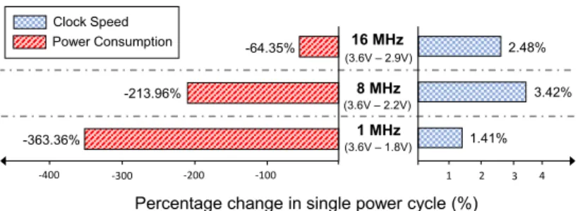
1 MHz 8 MHz 16 MHz 1 2 3 4 -100 -200 -300 -400 1.41% 3.42% 2.48%
Percentage change in single power cycle (%) (3.6V – 1.8V) (3.6V – 2.2V) (3.6V – 2.9V) -363.36% -213.96% -64.35% Clock Speed Power Consumption
Fig. 1. Impact of supply voltage variations on MSP430G2553 clock speed and power consumption in a single power cycle. Existing tools typically ignore these behaviors when modeling the energy consumption of TPC.
1 INTRODUCTION
Transiently-powered computers (TPCs) may rely on a great variety of energy harvesting mecha-nisms, often characterized by strikingly different performance and unpredictable dynamics across
space and time [10]. As much as using solar cells may yield up to 240𝑚W, but only at specific times
of the day and certain environmental conditions [23], harvesting energy from RF transmissions
solely produces up to 1𝜇W whenever the transmitter is sufficiently close [3].
Hardware and software must be dimensioned and parameterized according to these dynamics. Capacitors are used as ephemeral energy buffers. Smaller capacitors yield smaller device footprints and quicker recharge times, at the expense of smaller overall energy storage. The microcontroller units (MCUs) also feature numerous configuration parameters. For example, lower clock frequencies allow one to exploit larger operating ranges in supply voltage, but slow down execution. The MSP430-series MCUs run with supply voltages as low as 1.8V at 1 MHz, but are unable to run any lower than 2.9V at 16 MHz.
As TPCs increasingly employ separate capacitors to power the MCU or peripherals [25], the
ability to accurately forecast the energy cost of a certain fragment of code is key to decide on the size of capacitors powering the MCU and on its frequency settings. Peripheral operations may
often be postponed if their capacitors have insufficient energy [25], whereas the MCU coordinates
the functioning of the entire system. Accurate energy forecast information aids the efficient placement of systems calls that checkpoint the MCU state on non-volatile memory to cross periods
of energy unavailability [5,8,43]. Programmers may alternatively rely on task-based programming
abstractions that offer transactional semantics [16,36,38]. Thus, they need to know the worst-case energy costs of given task configurations to ensure completion within a single capacitor charge, or forward progress may be compromised.
Observation. Modeling energy consumption of TPCs is an open challenge [17,26,35]. Existing
tools are mainly developed for battery-powered embedded devices, which typically enjoy consistent energy supplies for relatively long periods. In contrast, capacitors on TPCs may discharge and recharge several times during a single application run. A single iteration of a CRC code may require
up to 17 charges and consequent discharges when harvesting energy from RF transmissions [43].
Single executions of even straightforward algorithms thus correspond to a multitude of rapid
sweeps of an MCU’s operating voltage range [8,43].
We experimentally observe that such a peculiar computing pattern causes severe fluctuations in
an MCU’s energy consumption. Fig.1shows example fluctuations we measure on an MSP430G2553
MCU running at 1 MHz in a single power cycle, that is, as it goes from the upper to the lower extreme of the operating voltage range. Power consumption varies significantly; it reduces by a
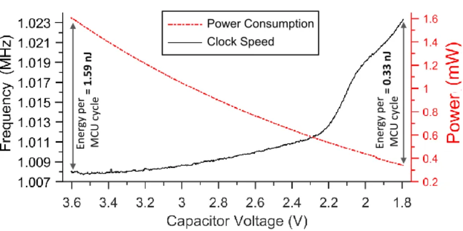
Ener gy per MCU cy cle = 1. 59 nJ Ener gy per MC U cy cle = 0 .3 3 nJ Power Consumption Clock Speed
Fig. 2. Impact of supply voltage variations on MSP430G2553 power consumption and clock speed. Energy being a product of power (red dotted line) and execution time, which is a function of clock speed (black solid line), the energy cost of a single MCU cycle varies by up to ≈5× depending on the instantaneous supply voltage.
factor of up to 363.36%. Clock speed also changes; it increases by a factor of up to 3.42%. This means the same instruction takes different times depending on the supply voltage.
The combined fluctuations of power and clock in Fig.1cause the energy cost of each MCU cycle
to drop by up to 5× in a power cycle. Fig.2shows this behavior as a function of supply voltage,
again in a single power cycle. Even for a single application run, as mentioned earlier, the system may require thousands of power cycles; the net effect thus accumulates in the long run.
Unlike dynamic frequency or voltage scaling [41,42] in mainstream platforms, these dynamics
happen regardless of the current system workload and the software layers have no control on them. Fluctuations in power consumption are exclusively due to the dynamics in supply voltage and clock speed. In turn, the latter are due to the design of the digitally-controlled oscillators (DCOs) that equip TPCs such as the MSP430-based ones. In fact, TI designers confirm that many of their MSP430-series MCUs employ DCOs that cause the clock speed to increase as the supply voltages
approaches the lower extreme1[31]. This yields better energy efficiency at these regimes, at the
cost of varying execution times.
Reasoning on such dynamic behavior is not trivial. For simplicity, a vast fraction of existing literature overlooks these phenomena [8,17,20,43]. Many systems are designed and parameterized in overly-conservative ways, by considering a constant power consumption no matter the supply voltage, and fixed clock speeds. We argue, however, that considering these dynamics is crucial, as their impact magnifies for TPCs with rapid and recurring power cycles.
Contribution. We demonstrate that it is practically possible to accurately model and concretely capitalize on these dynamics. As a result, we obtain significant performance improvements in a range of situations, exclusively enabled by considering phenomena that are normally not accounted
for. Following background material in Sec.2, our contribution is three-pronged:
(1) We empirically measure the impact of varying voltage supplies on clock speed and power consumption for all possible clock configurations, and derive an accurate energy model,
described in Sec.3. Analytically modeling these dynamics is difficult. Clock speed varies
as a result of the DCO design, discussed earlier. Power consumption varies according to a
nonlinear current draw by the MCU, caused by inductive and capacitative reactance of the clock module that uses internal resistors to control the clock speed.
(2) Our energy model enables the design and implementation of EPIC2, an automated tool that
provides accurate compile-time energy information, described in Sec.4. EPIC first augments
the source code with energy information at basic-block granularity. It then allows developers to tag a piece of code to determine best- and worst- case energy consumption.
(3) We present MSPsim++ in Sec.5, an integration of our energy model with MSPsim [20], a
widely used instruction set emulator based on static power and clock models. This is to cater for the several systems that leverage run-time information. MSPsim++ emulates the dynamic behaviors of supply voltage, clock speed, and power consumption on a per-instruction basis. This is the finest possible granularity without resorting to real hardware.
Benefits. We demonstrate the use of EPIC in two diverse scenarios. On one hand, we integrate
EPIC with HarvOS [8], an existing system support for TPCs. HarvOS decides on the placement
of system calls that possibly trigger a checkpoint to save the state on non-volatile memory until new energy is available. The accurate energy estimates of EPIC—used in place of the assumption of constant clock speed and power consumption in the original HarvOS—allow given workloads to complete with up to 50% fewer checkpointing interruptions. The energy saved from reducing checkpoints is then shifted to useful computation, resulting in up to ≈350% speedup in workload completion times. In specific cases, EPIC even indicates that the code may complete on a single charge with no need for checkpointing; this completely spares the corresponding overhead, which often surpasses the energy required by the application itself.
Next, we plug EPIC within CleanCut [17], a tool supporting task-based programming [17,38].
Such programming abstractions ensure transactional semantics; tasks are either completed when-ever energy is sufficient, or their partial execution has no effects. Howwhen-ever, tasks might accidentally be defined so that their worst-case energy cost exceeds the maximum available energy, impeding forward progress. Programmers use CleanCut to detect these cases, so they can, for example, split tasks into smaller units. Using EPIC with CleanCut to replace the assumption of constant clock and power allows one to ascertain that many of these warnings are, in fact, bogus. Programmers may thus avoid unnecessary program changes that ultimately hurt performance.
Conversely, we use MSPsim++ instead of the original MSPsim in MementOS [43], a different
system support for TPCs. MementOS uses MSPsim to determine the most efficient system-wide voltage threshold when to trigger a checkpoint. The voltage threshold identified with MSPsim++ is typically much smaller, as it is aware of the increase in energy efficiency as the supply voltage drops. For example, when running RSA encryption, MSPsim++ recommends a checkpointing threshold of 2.4V instead of 3.4V, resulting in up to one order of magnitude fewer checkpoints to complete its execution. The energy saved from sparing checkpoints is again shifted to useful computations, yielding up to more than 1000% speedup in workload completion time.
We conclude the paper by discussing limitations of our work in Sec.6, by surveying related work
in Sec.7and with concluding remarks in Sec.8.
2 BACKGROUND
We describe the factors that concur to determining the energy consumption of TPCs at a fundamental level, to investigate the dependencies affected by the dynamics of supply voltage.
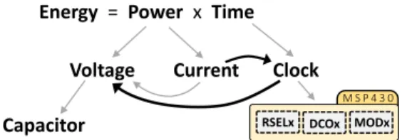
Calculating energy. Fig.3graphically depicts the dependencies among the relevant quantities.
Predicting energy consumption relies on precise values of both power consumption and execu-tion time, as their impact is multiplicative. In embedded MCUs, energy consumpexecu-tion is typically
Energy = Power x Time Voltage Current Clock
Capacitor RSELx DCOx MODx
M S P 4 3 0
Fig. 3. Dependencies among quantities determining energy consumption. The direction of the arrows depict the direction of dependency. Power consumption depends upon the input voltage and the current draw. The execution time depends on clock speed. As the supply voltage rapidly varies, additional dependencies are created, shown by black arrows, that perturb an otherwise constant behavior.
estimated by deriving the execution time from the number of clock cycles taken, while power consumption is calculated by multiplying a supposedly constant voltage supply with the current draw for a given MCU resistance.
Supply voltage, however, depends on the charge of the energy storage facility, which is most often a capacitor in TPCs. Due to their extensive usage in electronics, the accuracy of existing capacitor models—related to (dis)charging behavior of the capacitor and voltage drop between the plates—is well studied [27].
The current drawn by the MCU depends on both the supply voltage and the clock speed. While the former dependency is straightforward (V=IR), the latter stems from internal resistance typically
controlled through a clock-control register. Sec.3further discusses this aspect for MSP430-class
MCUs. These are arguably de-facto standard on TPCs [25,44] and represent the only case of
commercially-available embedded MCU with non-volatile main memory, which aids saving state across power cycles.
The time factor used to calculate the energy consumption depends on the actual clock speed. Embedded MCUs offer specific parameters to configure the clock speed. For example, MSP430-series
MCUs provide three parameters, called RSELx, DCOx, and MODx, as explained in Sec.3.
No More Constant Power × Time. Existing energy estimation tools [20,46] do model the
de-pendencies shown by grey arrows in Fig.3. For simplicity, they tend to overlook the dependencies
indicated by black arrows and consider constant values for the involved factors.
The same observation applies to many system solutions in TPCs [43]. As extensively discussed
in Sec.3, we experimentally observe that the assumption of constant power and execution time is
actually not verified in TPCs. The impact of this is significant in TPCs, as the supply voltage may potentially traverse the whole operational range multiple times during a single application run.
As the supply voltage varies wildly, a ripple effect creates that spreads the variability over time to clock speed and, in turn, to current draw. This essentially means that the phenomena traverse
the dependencies in Fig.3backward, eventually impacting both power consumption and execution
time. As a result, these figures are no longer constant, but their values change as frequently as the supply voltage delivered by a capacitor. Nevertheless, both figures ultimately concur to determine energy consumption.
In the next section, we describe the empirical derivation of an energy model that accounts for these phenomena.
3 ENERGY MODEL
We describe the methodology to derive models accounting for the dependencies shown by black
arrows in Fig.3. First, we discuss modeling the dependency between supply voltage and clock speed.
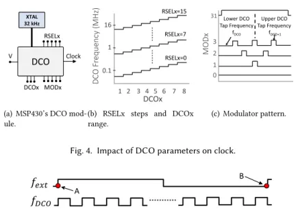
DCO RSELx V DCOx MODx Clock XTAL 32 kHz
16
1
0.1
RSELx=151 2 3 4 5 6 7 8
DC
O
Fr
equency
(MHz)
DCOx
RSELx=7 RSELx=03
2
1
0
MODx
Lower DCO Tap Frequency fDCO Upper DCO Tap Frequency fDCO+1 31(a) MSP430’s DCO mod-ule. DCO RSELx V DCOx MODx Clock XTAL 32 kHz 16 1 0.1 RSELx=15 1 2 3 4 5 6 7 8 DC O Fr equency (MHz) DCOx RSELx=7 RSELx=0 3 2 1 0 MODx Lower DCO Tap Frequency fDCO Upper DCO Tap Frequency fDCO+1 31
(b) RSELx steps and DCOx range. DCO RSELx V DCOx MODx Clock XTAL 32 kHz 16 1 0.1 RSELx=15 1 2 3 4 5 6 7 8 DC O Fr equency (MHz) DCOx RSELx=7 RSELx=0 3 2 1 0 MODx Lower DCO Tap Frequency fDCO Upper DCO Tap Frequency fDCO+1 31 (c) Modulator pattern.
Fig. 4. Impact of DCO parameters on clock.
𝑓
𝑒𝑥𝑡𝑓
𝐷𝐶𝑂 AB
Fig. 5. Clock frequency measurements. The number of clock cycles (𝑓𝐷𝐶𝑂) are counted between A and B, namely,
two consecutive low to high transitions of the external crystal oscillator 𝑓𝑒𝑥 𝑡.
0 1 2 3 4 5 Difference (%) 0 0.2 0.4 0.6 0.8 1 CDF (a) Frequency. 0 50 100 150 Difference (%) 0 0.2 0.4 0.6 0.8 1 CDF (b) Current. 1x 2x 3x 4x Difference (x) 0 0.2 0.4 0.6 0.8 1 CDF (c) Power.
Fig. 6. Impact of voltage supply variations on clock, current, and power for all DCO configurations. The x-axis shows the difference in the corresponding factor when the voltage drops from one extreme of the MCU’s operational voltage range to the other.
To make the discussion concrete, we target MSP430-class MCUs as arguably representative of TPC platforms, although our methodology applies more generally and has a foundational nature. These MCUs employ a 16-bit RISC instruction-set architecture with no instruction or data-cache, while application data always resides in and fetched from main-memory.
Once an energy model is derived for other MCUs, the design of the tools we describe in the remainder of the paper remains the same. The quantitative discussion that follows refer to the energy model we obtain for MSP430G2553 MCU, ; we find our conclusions to be equally valid for MSP430G2xxx MCUs, based on repeating the same modeling procedures.
3.1 Modeling Clock Drift
0 1 2 3 4 5 6 7 0 1 2 3 4 5 6 7 DCOx 1.2 1.45 1.7 1.95 2.2 2.45 2.7 2.95 3.2 3.45 Frequency (MHz) RSEL = 8 RSEL = 9 1.0% 1.54% 2.82% 1.65% 2.24% 3.53% 3.6 V 1.8 V
(a) Sensitivity of clock to voltage
0 2 4 6 8 10 # of Power Cycles 0 2000 4000 6000 8000 10000 12000
Unrepresented Clock Cycles
(b) Unrepresented clock cycles @ 8 MHz
Fig. 7. Clock behavior. (a) The sensitivity of clock to voltage increases for a given RSELx when the value of DCOx is increased, as well as across increasing RSELx values. The percentage values represent the difference in frequency between the two extremes of the operational voltage range; (b) The cup-shaped segments, with each cup corresponding to a single power cycle, show that the number of unrepresented cycle increases with the decreasing voltage of the capacitor. Charging times are omitted for brevity.
MSP430 clock module. As shown in Fig.4(a), MSP430 MCUs employ a digitally controlled
oscil-lator (DCO) that can be configured to deliver frequencies from only a few KHz up to 16 MHz. DCOs on MSP430 MCUs are configured using three parameters: RSELx, MODx, and DCOx, which are together hosted in two MCU registers called DCOCTL and BCSCTL1. RSELx stands for resistor-select and is used to configure the DCO for one of the sixteen nominal frequencies in the range 0.06 MHz to 16 MHz. DCOx uses three bits to further subdivide the range selected by
RSELx into eight uniform frequency steps as shown in Fig.4(b). Finally, MODx stands for DCO
modulator, and enables the DCO to switch between the configured DCOx and the next higher frequency DCOx+1. The five bits of MODx define 32 different switching-frequencies, as depicted in Fig.4(c), to achieve fine-grained clock control.
Measurement procedure. Measuring clock speeds is challenging as the oscilloscope probes, when hooked to the clock pin, perturb the DCO impedance. This results in fluctuating measurements.
We thus employ a verified software-based measurement approach used by Texas Instruments for
DCO calibration [29]. It consists in counting the number of MCU ticks within one clock cycle of an
external crystal oscillator, as shown in Fig.5. In MSP430 MCUs, the external crystal oscillator is a very stable clock source offering a frequency of 32.768 KHz. Since the time period of this oscillator is greater than the time period of MCU ticks, we use it to count the number of MCU ticks during its period.
We initialize the Capture/Compare register of Timer_A in the MSP430 to Capture mode. The output of DCO is wired to this register and captures the value of Timer_A when a low-to-high transition occurs on the reference signal, that is, the external oscillator. The captured value is the number of clock cycles between two consecutive low-to-high transitions of the reference signal. Empirical model. To comprehensively model the clock behavior, we sweep the parameter space and empirically record the range of frequencies generated by different DCO configurations.
Altogether, 4096 discrete DCO frequencies can be generated using all possible combinations of
RSELx, DCOx, and MODx. As observed in Fig.2, however, the supply voltage impacts the actual
clock speed given a certain clock configuration. For each of these 4096 configurations, we evaluate this impact for the entire operational range of the MCU at 0.001V intervals, and record over 69,888 unique frequencies. These fine-grained measurements allow us to analyze the sensitivity of the
clock to supply voltage, and ultimately derive an accurate model. Our analysis is centered around two key question: i) is the sensitivity of changes in clock speed to changes in supply voltage consistent across all frequencies? and ii) how essential is it to model the clock behavior?
To answer the first question, in Fig.6(a)we plot the cumulative distribution of the percentage
difference in clock speed when the voltage drops from one extreme of the MCU’s operational voltage range to the other, across all possible DCO settings that determine a given MCU frequency. The
arc-shaped curve in Fig.6(a)implies that the sensitivity of changes in clock speed, which ranges
from ≈0% to ≈4.5% (x-axis), is not consistent across all frequencies.
We note, however, that this apparent inconsistency is not the outcome of a random clock behavior,
but a predictable DCO artefact that is observable in most low-power MSP430 MCUs. Fig.7(a)shows
how clock speed changes for a given RSELx when DCOx increases, as well as across increasing RSELx values, for the two extremes of the operational voltage range. TI designers confirm this DCO drift pattern, which is conceded for power conservation and is specified as DCO tolerance. The exact circuit design causing this behavior is protected by intellectual property [32].
To answer the second question, we quantify the number of clock cycles that a constant clock model, that is, one that does not incorporate the changes in clock speed as the voltage drops, would
not account for. Fig.7(b)shows that this figure increases linearly with every power cycle; more
than 10K clock cycles would be unrepresented in only ten power cycles. This could be extremely critical for correctly designing and dimensioning systems that may undergo countless power cycles throughout their lifetime.
3.2 Modeling Dynamic Power Consumption
Besides affecting the time component of the energy equation, changes in supply voltage and clock speed also impact current draw, and hence power consumption. A precise current model is thus crucial in determining accurate power consumption, as instantaneous power consumption is a product of voltage and current. While the amount of current drawn by the MCU naturally decreases with voltage and can be calculated using Ohm’s law, measuring the impact of changes in clock speed on current draw is not immediate.
In MSP430 MCUs, clock speed is mainly controlled by the DCO impedance, which is controlled using the parameters described earlier. This results in varying amounts of current drawn at different frequencies. However, the impedance of the DCO, which can be modeled as an RLC circuit, cannot be derived theoretically since the values of ohmic resistance and reactance are unknown. Measurement procedure. Similar to the clock model, we employ an empirical approach to model the cumulative impact of changes in supply voltage and clock speed on current consumption. Our measurement setup includes a 0.1𝜇 ampere resolution multimeter, which measures and automati-cally logs the current drawn by the MCU.
Since the correctness of measurements is critical to derive an accurate model, our approach also caters for the burden voltage—the voltage drop across the measuring instrument. We add the burden
voltage (𝑉𝑏) to the supply 𝑉𝑠. However, this leads to the current measurements of the MCU at a
higher voltage (𝑉𝑏+𝑉𝑠), whereas we need the current draw precisely at 𝑉𝑠. As we know the values
of 𝑉𝑏and the the current draw (𝐼𝑚), we calculate the resistance (𝑅𝑖) of the measuring instrument.
We then simply calculate the current draw of the MCU as 𝐼𝑚𝑐𝑢 = 𝐼𝑚−
𝑉𝑏
𝑅𝑖.
Empirical model. Unlike the sensitivity of clock to changing supply voltage in Fig.6(a), the
current’s sensitivity to changes in clock speed and supply voltage is quite consistent and above 100% for a large fraction of frequencies, as shown in Fig.6(b).
The inconsistent behavior for less than 20% observations is due to DCO’s unstable behaviors for very slow frequency configurations (below 1 MHz), which are typically neither calibrated nor
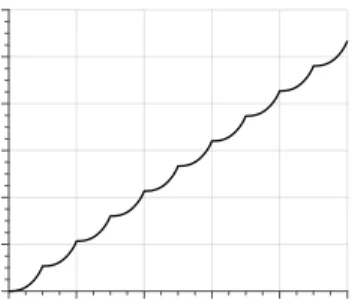
Fig. 8. Model representations and their behavior compared to empirical measurements @ 8 MHz. Higher precision lookup tables follow closely the actual measurements. The polynomial model rests within a 2% error bound.
used with MSP430 MCUs [28]. Fig.6(c)highlights the multiplicative impact of changes in supply
voltage and current on an MCU’s power consumption. Power consumption may vary as much as 3.5× within a single power cycle. This demonstrates that existing tools, as they fail to model such behaviors, tend to be provide inaccurate inputs to the design and dimensioning of TPCs.
3.3 Model Representation
We consider two choices to represent the results of our measurements for either model. Either we
use a lookup table or train a model with RSELx, DCOx, MODx and supply voltage (V𝑠) as inputs.
The former is of course, exhaustive, but unlikely to fit on an embedded MCU with little main
memory, for example, to be used at run-time to implement energy-adaptive behaviors [12,14]. For
instance, a large lookup table with a precision of three decimal places and a small lookup table with a precision of one decimal place would consume 28 MB and 288 KB in main memory, respectively. We thus also explore the derivation of a compact model based on linear regression able to fit within the limited memory budget of embedded MCUs. We observe that a degree 7 polynomial is sufficient to fit a model with error bound to ±6%. This can readily be reduced to ±1% with a degree 3 polynomial when used for common DCO frequencies such as 1 MHz, 8 MHz, and 16 MHz.
Figure8highlights the behavior of these different representations of the clock model during a
single power cycle. A large lookup table with 0.001V precision accurately follows the measurements, whereas a small look up table with 0.1V precision predictably mimics a step function. The polynomial model, in this particular setting, achieves an average error below 2%.
What model representation to employ is, therefore, to be decided depending on desired accuracy and intended use. Compile-time or off-line analysis may use the lookup table representation, which faithfully describes the results of our measurements. Whenever the models are to be deployed on an embedded MCU with little memory, the polynomial model is way easier on memory consumption.
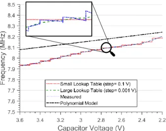
Fig. 9. Dynamic vs. constant energy models @ 8 MHz. Depending on supply voltage, a constant model may overestimate (shaded blue region) or underestimate (shaded red region) the energy available with a single discharge of a 10𝜇F capacitor.
3.4 Summary of Findings
We conclude that modeling these dynamic behaviors is essential for designing and dimensioning TPC systems, as accounting for them may lead to improved performance. Before providing
quan-titative evidence of this in Sec.4and Sec.5, we reason about the general impact of the dynamic
model described above when compared with a range of assumed constant models in Fig.9.
The green line in the middle shows the accurate prediction of energy consumption during a single power cycle by our model. The shaded blue region represents the range of constant models that overestimate energy consumption [8,17,20,43]. Most existing tools lie on the left-most, dashed blue line as they are designed for worst-case analysis, namely, they compute energy consumption by assuming a constant input voltage at 3.6V. Systems designed and configured with these models may significantly under-perform; for example, an overestimation of energy consumption may
lead to overly conservative placements of expensive checkpoint calls in the code [8,43], as we
demonstrate in both Sec.4and Sec.5.
Differently, the shaded red region below the green line shows the range of constant models that would underestimate energy consumption, by considering a constant lower voltage within the MCU’s operational range. TPC systems based on such models may fail; for example, an underesti-mation of energy may lead to non-termination in task-based systems, where a wrongly-defined
task may require more energy than a capacitor can store [17].
4 EPIC
Based on our energy models, we develop EPIC: a compile-time analysis tool that accurately pre-dicts energy consumption of arbitrary code segments. Existing solutions employ time-consuming
laboratory techniques [8], and yet they overlook the impact of variations in supply voltage. EPIC
provides this information in an automated fashion and by explicitly accounting for such dynamics.
4.1 Workflow
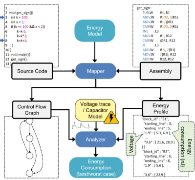
Mapper Analyzer Source Code Control Flow Graph Energy Model Assembly Energy Profile get_sign: SUB.W #4, R1 MOV.W #100, 2(R1) MOV.W #1, @R1 CMP.W #100, 2(R1) JNE .L3 MOV.B #1, R12 CMP.W @R1, R12 JL .L3 ADD.W #-5, 2(R1) MOV.W 2(R1), R12 ADD.W R12, R12 1… 2voidget_sign(){ 3 intk = 100; 4 intx = 1; 5 if (k == 100 && x < 2){ 6 k=k-5; 7 k=k*2; 8 k=k+3; 9 } 10 } 11voidmain(){ 12 get_sign(); 13 } "block_id" : “B1", "starting_line" : 3, "ending_line" : 5, "1.9" : [ 5.3, 6.9 ], ... "3.6" : [ 21.6, 28.0 ] } { "block_id" : "B2", "starting_line" : 6, "ending_line" : 8, "1.9" : [ 5.6 ], ... "3.6" : [ 22.9 ] Voltage trace / Capacitor Model Energy Consumption (best/worst case) Ener gy consumption (nJ ) V olt ag e
Fig. 10. EPIC code instrumentation process. The mapper maps the assembly instructions to the corresponding basic blocks in the source code and outputs a CFG and energy profile based on the models of Sec.3. The analyzer traverses the CFG to compute best- and worst-case estimates for a given fragment of code and capacitor size.
Mapper. Inputs for the mapper module are the empirical energy model, a portion of the source code marked by developers for analysis, and the corresponding assembly code generated for a specific platform. Instructing the compiler to include debugging symbols in the assembly allows the mapper to establish a correspondence between each assembly instruction and the corresponding source code line [34,46]
The mapper initially analyzes the assembly code to find the basic blocks at the level of source code that corresponds to a given set of assembly instructions. Using this mapping and information on the number of MCU cycles required by each assembly instructions, EPIC computes the total number of MCU cycles per basic block at the level of source code. Such a mapping process is non-trivial; we defer a more detailed discussion to Sec.4.2.
Next, the mapper relies on the empirical energy model to predict the energy consumption of each basic block. The output of this step is a separate file, called energy profile, which contains the energy consumption of each basic block at arbitrary supply voltages within the operational range of the target MCU. We store this information in JSON format to facilitate parsing by compile-time tools relying on the output of EPIC. Finally, the mapper also generates the control-flow-graph (CFG) of the code using ANTLR.
Analyzer. The goal of the analyzer is to determine best- and worst-case estimates of energy consumption for each node in the CFG. To that end, the analyzer takes as input the energy profile output by the mapper and a trace of supply voltage values used to determine which value to choose from the energy profile for a particular basic block. Two choices are available for this: either using a capacitor model that simulates the underlying physics and specific (dis)charging behaviors, or relying on a user-provided energy trace that indicates the state of capacitor’s charge over time.
Similar to other compile-time tools, the best- and worst-case energy consumption estimates are the best output EPIC can provide. Nevertheless, there are cases where these estimates depend on run-time information; for example, in the presence of loops whose number of iterations is not known at compile time. If a user-specified piece of code also includes any of these programming constructs, EPIC prompts the user for ascertaining the number of loop iterations to be considered in a given analysis.
4.2 Finding MCU Cycles per Basic Block
Established techniques exist to determine a mapping between basic blocks at the level of source
code and assembly instructions, for example, as used in simulation tools such as PowerTOSSIM [46]
and TimeTOSSIM [34]. These techniques, however, do not accurately handle cases where a given
basic block of source code may correspond to the execution of a variable number of instructions in assembly; therefore, a single node in the CFG is translated into multiple basic blocks at the assembly level. Short-circuit evaluation, for loops, and compiler-inserted libraries are examples where issues manifest that may cause a loss of accuracy in energy estimates.
To handle these cases, EPIC further dissects the mapping process to extract additional information useful to reason on the energy consumption of a given basic block, as described below.
Short-circuit evaluation. These include arbitrary concatenations of logical operators, such as “&&” or “||”, where the truth value of a pre-fix determines the truth value of the whole expression, independent of the truth value of the post-fix. In these cases, the assembly code generated by the compiler skips the evaluation of the post-fix part of the expression as soon as the pre-fix determines the truth value of the whole expression.
To handle these cases, the mapper reports the energy consumption of all possible evaluations
of the statement involving these operators. This is shown in the energy profile of Fig.10for the
ifstatement at line 5 of the source code. Two separate values are reported for the corresponding
basic block (B1), one for only the pre-fix and one for the complete evaluation of the expression. This information is then useful for the analyzer module, which may choose the appropriate value depending upon the type of analysis required. For example, when considering the best-case energy consumption, the analyzer considers the energy consumption for executing the minimal pre-fix that determines the truth value. Differently, the analyzer accounts for the energy consumption of executing every sub-expression when computing the worst case.
Loops using for. The execution of these loops may incur a different number of MCU cycles at the first or at intermediate iteration(s). This is because the initialization of the loop variable is only performed at the first iteration, whereas all other iterations incur the same number of MCU cycles as they always perform the same operations; for example, incrementing a counter and checking its value against a threshold.
The mapper accurately identifies the set of instructions needed for these two different types of execution of the for(;;) statements, and reports them in the energy profile as two separate entries for the corresponding basic block. The analyzer then utilizes this information to accurately calculate the energy consumption of different loop iterations.
Compiler-inserted functions. For programming constructs that are not supported natively in hardware, such as multipliers and floating point support, compilers insert their own library functions to emulate the desired functionality in software. However, the execution-time of these library functions depends on their arguments. Since there are only a handful of such library functions typically, we address this problem by profiling these with arbitrary inputs as function arguments and record their best- and worst-case energy consumption.
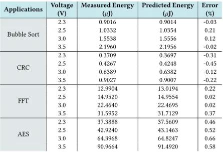
Table 1. EPIC accuracy.
Voltage Measured Energy Predicted Energy Error Applications (V) (𝜇J) (𝜇J) (%) 2.3 0.9016 0.9014 -0.03 2.5 1.0332 1.0354 0.21 3.0 1.5538 1.5556 0.12 Bubble Sort 3.5 2.1960 2.1956 -0.02 2.3 0.3709 0.3697 -0.31 2.5 0.4267 0.4248 -0.45 3.0 0.6389 0.6382 -0.12 CRC 3.5 0.9027 0.9007 -0.22 2.3 12.9904 13.0194 0.22 2.5 14.9520 14.9554 0.02 3.0 22.4640 22.4695 0.02 FFT 3.5 31.5952 31.7129 0.37 2.3 37.3888 37.5609 0.46 2.5 42.9240 43.1463 0.52 3.0 64.3968 64.8247 0.66 AES 3.5 90.9664 91.4920 0.58
These specific design choices enables EPIC to make only a single pass of the entire application code to predict energy consumption. This improves scalability, as EPIC’s runtime only increases linearly with the application size. Assessing the utility of EPIC for complex architectures, such as MCUs with instruction pipelines and caches, is a potential challenge of unknown complexity and we leave it as a future work.
We next evaluate the accuracy of energy profile information returned by EPIC across four benchmark applications, before employing the entire EPIC workflow for compile-time analysis in two concrete cases.
4.3 Microbenchmarks
We first investigate the accuracy of the energy profile information returned by the mapper module in EPIC. In turn, this depends on i) the accuracy of the empirical energy model described in Sec.3, and ii) the effectiveness of the mapping techniques between source code and assembly code illustrated in Sec.4.2. Understanding whether the energy profiles are accurate is a stepping stone to investigate the use of EPIC in a concrete case study.
Our benchmarks include open-source implementations of Bubblesort, CRC, FFT, and AES, which
are often employed for benchmarking embedded systems [22], and specifically system support for
TPCs [5,33,43]. We run each application on real hardware at different supply voltages and record a per-basic-block trace of execution time and current draw to compute the energy consumption.
Table1compares the results returned by the mapper module of EPIC at different supply voltages
with the empirically measured ones on an MSP430G2553 running at 8 MHz. The error is generally well below 1%. The results demonstrate that the information to the analyzer module is accurate, as a result of the accuracy of the empirical model and the mapping between source code and assembly we adopt.
4.4 EPIC with HarvOS
We integrate EPIC with HarvOS [8], an existing system support for TPCs. HarvOS relies on
compile-time energy estimates to insert system calls—termed triggers—that possibly execute a checkpoint whenever a device is about to exhaust the available energy. The triggers include code to query the
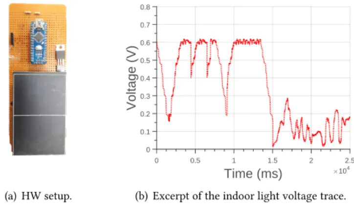
(a) HW setup. Time (ms) #104 0 0.5 1 1.5 2 2.5 Voltage (V) 0 0.1 0.2 0.3 0.4 0.5 0.6 0.7 0.8
(b) Excerpt of the indoor light voltage trace.
Fig. 11. Voltage trace from indoor light using a mono-crystalline solar panel.
state of the energy buffer for deciding whether or not to checkpoint. Checkpoints are costly in energy and additional execution time. Nonetheless, regardless of whether a checkpoint takes place,
these calls represent an overhead, as merely querying the energy buffer consumes energy [43].
In HarvOS [8], the placement of trigger calls is based on an efficient strategy that requires
a worst-case estimate of the energy consumption of each node in the CFG. Similar to existing literature, HarvOS normally employs a manual instrumentation process based on a static energy consumption model, namely, overlooking the dynamic behavior of power consumption and clock speeds. We use EPIC to substitute for such manual instrumentation process.
Setup. We use two applications: i) an Activity Recognition (AR) application that recognizes human
activity based on sensor values, often utilized for evaluating TPC solutions [16,36], and ii) an
implementation of the Advanced Encryption Standard (AES), which is one of the benchmarks used
in HarvOS to investigate its efficiency [8]. We execute EPIC by relying on two different types of
voltage traces as an input to the analyzer module.
First, we use a fundamental voltage trace often found in existing literature [7,33,43,51]. The device boots with the capacitor fully charged, and computes until the capacitor is empty again. In the meantime, the environment provides no additional energy. Once the capacitor is empty, the environment provides new energy until the capacitor is full again and computation resumes. This energy provisioning pattern generates executions that are highly intermittent, namely, executions that most paradigmatically differentiate TPCs from other embedded and mainstream platforms. Further, this profile is representative of a staple class of TPC applications based on wireless energy transfer [9]. With this technology, devices are quickly charged with a burst of wirelessly-transmitted energy until they boot. Next, the application runs until the capacitor is empty again. The device rests dormant until another burst of wireless energy comes in. We call this trace the decay trace.
Second, we use a voltage trace collected using a mono-crystalline high-efficiency solar panel [48],
placed on a desk and harvesting energy from light in an indoor lab environment, as shown in Fig.11.
We use an Arduino Nano [4] to log the voltage output across the load, equivalent to the resistance
of an MSP430G2553 in active mode, attached to the solar panel. We call this trace the light trace. Results. By comparing the features and the performance of HarvOS-instrumented code using the manual energy profiling technique in the original HarvOS or EPIC, based on an MSP430G2553 running at 8MHz, we draw the following observations:
(1) Using EPIC, the number of trigger calls inserted by HarvOS in the original code reduces; (2) A more accurate code instrumentation due to EPIC leads to fewer checkpointing interruptions.
Table 2. Features and performance of HarvOS-instrumented code with and without EPIC. # of trigger calls # of checkpoints Speedup in completion
Application Manual EPIC Manual EPIC time (%)
Decay Trace AR 2 1 85 42 51.66 AES 3 0 2 0 354.97 Light Trace AR 2 1 64 32 49.35 AES 3 0 1 0 203.31
The first two columns in Table2show the results of the instrumentation process when using the
smallest capacitor size needed to complete the given workloads. We consider this as TPCs typically prefer smaller capacitors as energy buffer, because they reach the operating voltage more quickly and yield smaller device footprints. However, if the capacitor is too small, a system may be unable to complete checkpoints, ending up in a situation where applications cannot make any progress.
For the AR application, Table2indicates that EPIC’s accurate energy estimates halve the number
of trigger calls that HarvOS places in the code. This reduction occurs due to EPIC’s ability to accurately model the varying number of clock cycles at different voltages that a static model would not consider. As the voltage of the capacitor decreases, the speed of the clock increases. This results in more clock cycles becoming available per unit of time at lower supply voltages. Not accounting for such dynamic behavior significantly underestimates the number of clock cycles available within a single time unit in conditions with low supply voltages.
The results for AES instrumentation are revealing: based on the energy estimates provided by EPIC, HarvOS decides to place no trigger calls. This means EPIC indicates that the energy provided by the capacitor is sufficient for the AES implementation to complete in a single power cycle, and thus no checkpoints are ever necessary. This sharply contrasts the outcome of the HarvOS compile-time analysis whenever based on the assumption of constant power consumption and clock speed. In that case, HarvOS would still place three trigger calls within the AES code, uselessly incurring the corresponding overhead. This shows how not accounting for the dynamic behaviors represented by our energy model profoundly misguides compile-time analyses.
The impact of the trigger call placement with or without EPIC has marked consequences when
running the instrumented applications. The third and fourth columns in Table2show the
corre-sponding results for either voltage trace. The AR application instrumented by HarvOS based on the energy estimates of EPIC completes the execution with nearly 50% fewer checkpoints. Similarly, the successful completion of the AES implementation without a single checkpoint confirms the validity of the energy estimates of EPIC, which prompted HarvOS not to place any trigger call.
Checkpoint operations are extremely energy consuming, as they incur operations on non-volatile memory. Fewer checkpoints allow the system to spend the corresponding energy budget in useful computation cycles, which are otherwise wasted due to inaccurate insertion of trigger calls in the original HarvOS. Thus, the system progresses faster towards the completion of the workload. The
right most column in Table2quantifies the benefits in terms of speedup of completion time for the
given workload, primarily enabled by correct dimensioning of HarvOS using EPIC.
Fig.12further investigates the execution of either application at increasing capacitor sizes. These results affirm that the benefits of using EPIC within HarvOS are not just limited to the smallest
capacitor that ensures completion of a given code. The apparent outlier at 40uF in Fig.12(b)is due
to a specific behavior of HarvOS whenever larger capacitors simultaneously yield a change in the placement of trigger calls and in their overall number [8]. For the AR application, the corresponding
Capacitor (uF)
15 20 25 30 35 40 45 50# of checkpoints
0 20 40 60 80 100 120 Manual EPIC(a) AR with decay trace.
Capacitor (uF)
10 20 30 40 50# of checkpoints
0 20 40 60 80 100 120 Manual EPIC(b) AR with light trace.
Capacitor (uF)
5 10 15 20 25 30 35# of checkpoints
0 1 2 3 4 5 Manual EPIC(c) AES with decay trace.
Capacitor (uF)
5 10 15 20 25 30 35# of checkpoints
0 1 2 3 4 5 Manual EPIC(d) AES with light trace.
Fig. 12. HarvOS results. The benefits of using EPIC within HarvOS apply across different capacitor sizes.
speedup in completion time range from 14% at 35uF with the decay trace, to 159% at 40uF using
the light trace. For the AES implementation, the figures in Table2already show the performance
range, as no checkpoints are needed using capacitors larger than 20uF.
Finally, Fig.12also shows that in a number of situations, the compile-time instrumentation
generated by HarvOS when using the energy estimates of EPIC yields an operational system at much smaller capacitor sizes, as compared with the original HarvOS. The cost for the overly-conservative estimations in the latter, based on static power consumption and clock speeds, materializes in the inability to make any progress in these applications when using small capacitors. In contrast, EPIC captures the dynamic behavior of these figures and offers accurate estimations to HarvOS; this results in more informed decisions on trigger call placement and on whether to checkpoint when executing a trigger call.
4.5 EPIC with CleanCut
An alternative to using automated placement of trigger calls is to employ task-based programming abstractions offering transactional semantics [16,36,38]. Programmers are to manually define tasks that are guaranteed to either complete by committing their output to non-volatile memory or to have no effect on program state.
CleanCut [17] is a compile-time tool that helps programmers using these abstractions identify
non-termination bugs. These exist whenever a task definition includes execution paths whose energy cost exceeds the maximum available energy, based on capacitor size. In these cases, if no
Table 3. CleanCut non-termination bug warnings with and without EPIC. Application Task boundaries Paths CleanCut warnings EPIC warnings AR 4 147 8 0 RSA 4 8 3 0 CF 11 25 0 0 CEM 11 20 0 0
new energy is harvested while the task executes, that may never complete and thus the program ends up in a livelock situation, always resuming from the task beginning.
CleanCut relies on an energy model obtained through hardware-assisted profiling. The model estimates the energy consumption of each basic block at near maximum voltage supply, to avoid underestimations. The estimates are then convoluted across the possible execution paths in a task to find energy distributions for individual tasks. Based on this, CleanCut returns warnings whenever it suspects a non-termination bug. Programmers must then defend against these; for example, by refactoring the code to define shorter tasks. This is not just laborious, but also detrimental to performance, as every task boundary incurs significant energy overhead due to committing a task’s output on non-volatile memory.
Colin et al. [17] argue that an analytical model may provide more accurate warnings, but was
out of scope. Using EPIC with CleanCut, we prove this argument. For long execution paths in a task that use the capacitor to near depletion, the difference between the actual used energy—accurately modeled by EPIC—and CleanCut’s estimations obtained as described above, can be significant. This results in false positives, that is, non-termination bugs are suspected for paths that may safely complete with the given energy budget. Such warnings simply do not appear using EPIC. Setup. We use the same applications as in CleanCut [17]: i) an Activity Recognition (AR) application similar to Sec.4.4, ii) a Cuckoo Filter (CF) that efficiently tests set membership, iii) a Coldchain Equipment Monitor (CEM) application, and iv) an implementation of the RSA algorithm.
The placement of task boundaries is the one of CleanCut [17]. We then estimate the energy
consumption of every possible execution path in a task using CleanCut with EPIC, compared with CleanCut using a synthetic model that safely approximates that of CleanCut, whose hardware and source code are not available. This model follows the recommendation that the energy consumption
of each basic block should be estimated near the maximum voltage to avoid underestimations [17].
We use a 10𝜇F capacitor, which can be found on Intel WISP 4.1 devices, and consider an MSP430G2553 running at 8 MHz.
Results. Table3summarizes our results, which are further detailed in Fig.13. By comparing how
CleanCut and CleanCut using EPIC build up the energy estimates for a task, we note that the two start identical, but as paths become longer and nears the capacitor’s limit, CleanCut starts to overestimate. This is because it uses the same energy model for every basic block, regardless of where it appears on the path.
The results for the AR application in Fig.13(a)indicate that CleanCut returns eight false positives, in that it estimates the energy consumption of those paths to exceed the available capacitor energy. Developers would then need to break those tasks in smaller units, investing additional design and programming effort, and causing increased overhead at run-time due to more frequent commits to non-volatile memory at the end of shorter tasks. This is not the case with CleanCut using EPIC, which verifies that the same execution paths may complete successfully. This means the task placement includes no non-termination bugs; therefore, developers need not to spend any
5 10 15 20 Path 0 10 20 30 40 50 60 Energy (uJ) 2 2.5 3 3.5 Capacitor Voltage (V) CleanCut CleanCut + EPIC Device Capacity
(a) Activity Recognition (AR).
1 2 3 4 5 6 7 8 Path 0 10 20 30 40 50 60 Energy (uJ) 2 2.5 3 3.5 Capacitor Voltage (V) CleanCut CleanCut + EPIC Device Capacity (b) RSA. 0 5 10 15 20 25 Path 0 10 20 30 40 50 60 Energy (uJ) 2 2.5 3 3.5 Capacitor Voltage (V) CleanCut CleanCut + EPIC Device Capacity (c) Cuckoo Filter (CF). 5 10 15 20 Path 0 10 20 30 40 50 60 Energy (uJ) 2 2.5 3 3.5 Capacitor Voltage (V) CleanCut CleanCut + EPIC Device Capacity (d) CEM.
Fig. 13. CleanCut results. Using EPIC allows CleanCut to avoid false positives when looking for non-termination bugs.
additional effort and the system runs with better energy efficiency. Similar considerations apply to the case of the RSA algorithm, wherein CleanCut returns three false positives, as shown in Fig.13(b).
In the case of CF, processing is generally lighter compared to AR and RSA. Further, the existing task definition includes very short tasks already. As a result, the estimates of CleanCut and CleanCut
using EPIC are close to each other, as shown in Fig.13(c)No warnings for possible non-termination
bugs are returned in either case. Similar considerations apply also to the CEM application, whose results are shown in Fig.13(d).
CleanCut also provides a task boundary placer that automatically breaks long tasks. We cannot evaluate the impact of EPIC there, since the implementation is not available, but we argue that the benefits would be even higher. In fact, CleanCut’s placer is actively trying to bring task definitions to their optimal energy point, that is, closer to the capacitor limit. This is precisely where the difference in estimates between CleanCut and CleanCut with EPIC is maximum. Thus, the probability of paths landing in the region where CleanCut declares a task to be too long, but CleanCut using EPIC says the opposite, is likely higher compared to checking a manual placement.
5 MSPsim++
While compile-time analysis is important early on, testing down the road may necessitate cycle-accurate emulation to understand the run-time behavior.
We demonstrate the role of our energy models in this context within MementOS [43], an existing system support for TPCs that heavily relies on emulation to determine when a checkpoint is to be taken. Enabling this investigation is MSPsim++, an extension to the existing MSPsim
emulator [20] for MSP430 MCUs. Our analysis reveals the enormous discrepancies that might arise
in the performance of MementOS-supported applications by disregarding the dynamic behaviors of power consumption and clock speed.
5.1 Design
MSPsim is a widely used Java-based instruction level emulator for MSP430-based platforms. Its energy prediction model is based on static power consumption and clock speed. We replace these
with our own energy model, described in Sec.3, and refer to this extension as MSPsim++. The
capacitor model we use is borrowed from MementOS [43].
Computing the energy figures during an execution proceeds as follows. At the conclusion of each instruction execution, MSPsim++ subtracts the energy consumed by its execution from the capacitor. Next, it calculates the new supply voltage based on the capacitor model, and uses the new supply voltage value as the index into a table-based model representation at 0.1V resolution, as
explained in Sec.3.3. With the updated power consumption and clock speed, MSPsim++ executes
the next instruction. This means MSPsim++ emulates the dynamic behaviors of supply voltage, power consumption, and clock speed on a per-instruction basis. In an instruction-level emulator, this is the finest possible granularity.
Cycle-accurate emulation does not suffer from the potential inaccuracies in mapping source code
to assembly and back, described in Sec.4.2. MSPsim++ executes the exact same binary instructions
the real hardware executes. Therefore, our model integration in MSPsim++ is inherently more accurate than then compile-time results illustrated in Table1.
5.2 MSPsim++ with MementOS
MSPsim++ replaces the original MSPsim in MementOS. Using MSPsim++, we seek to understand the impact of modeling the dynamic behaviors of power consumption and clock speed on MementOS-supported applications.
Setup. MementOS uses checkpointing to protect a program from state losses due to energy depletion. The decision to checkpoint is based on a voltage threshold obtained through repeated emulation experiments and user-supplied voltage traces. These experiments use MSPsim to try and execute a MementOS-supported program with progressively decreasing thresholds to trigger checkpoints. This procedure returns the lowest threshold leading to completion of the program, with what is estimated to be the minimum number of required checkpoints.
Our two benchmarks use the same code base as the original MementOS [43], and are3: i) Cyclic
Redundancy Check (CRC) that computes a CRC16-CCITT checksum over a 2 KB region of flash memory, and ii) RSA cryptography that uses iterative left-to-right modular exponentiation of multiple-precision integers to encrypt a 64-bit message under a 64-bit public key and 17-bit exponent. In both cases, the results we discuss next use the “function call” strategy to inline the calls that
possibly checkpoints [43]. We obtain similar results using other MementOS strategies. Similarly,
these two benchmarks provide sufficient insights to generalize our conclusions. Although we evaluated many other applications, their results did not offer any newer insights.
3The results in [43] are not repeatable because neither the specific hardware platform nor the tools used for integration of MementOS with MSPsim are supported anymore. We contacted the hardware supplier and the MementOS developers, who encouraged us to apply the corresponding upgrades in the hardware and software tool-chain.
Table 4. Parameter setting and performance of MementOS applications with MSPsim or MSPsim++.
Vthresh (V) # of
checkpoints
Speedup in completion
Apps MSPsim MSPsim++ MSPsim MSPsim++ time (%)
Decay Trace CRC 3.0 2.3 64 9 392.88 RSA 3.4 2.4 42 3 152.76 Light Trace CRC 3.1 2.4 9 2 715.16 RSA 3.3 2.2 4 0 1037.43
We analyze the behavior of MementOS using either MSPsim or MSPsim++. We expect the voltage threshold determined at the end of these emulation experiments to be significantly lower using MSPsim++, since it recognizes the gain in clock speed and reduction in power consumption as the
voltage supply drops. We use the same decay and light traces used in Sec.4.4as input.
Results. The outcome of our investigation leads us to the following observations when using an MSP430G2553 running at 8MHz:
(1) MSPsim++ causes MementOS to use lower voltage thresholds to trigger a checkpoint; (2) Lower voltage thresholds reduce the run-time checkpointing overhead, shifting the energy
budget to useful computations.
The two left-most columns in Table4are obtained by considering the smallest capacitor size
where MementOS using MSPsim or MSPsim++ is operational.
The voltage thresholds confirm our hypothesis; as the original MSPsim does not model the dynamic behaviors of power consumption and clock speeds, the corresponding thresholds are overly conservative. Intuitively, with this configuration, MementOS would trigger a checkpoint too early: the execution might continue and a checkpoint be triggered later, once the supply voltage dropped further, and still complete successfully. In contrast, MSPsim++ returns lower voltage thresholds due to a more accurate modeling of energy consumption. A lower threshold means that part of the energy budget may be shifted from checkpointing operations to useful computations, as the checkpointing can be delayed until the capacitor voltage reaches a lower value.
This behavior shows in the the next three columns of Table4. Lower thresholds enable the
system to complete the application execution with up to one order of magnitude fewer checkpoints. As a result, available energy is rather spent for useful computations, thus making faster progress towards the completion of the workload. The corresponding speedup reaches more than 1000%.
Fig.14confirms that these improvements apply across different capacitor sizes. The difference in
voltage thresholds is less pronounced as the capacitor size increases. A little analogy may help: say a capacitor is akin to a water reservoir, and voltage represents the vertical level of water. With bigger capacitors (reservoirs), even a small difference in voltage may correspond to a large amount of energy (water). Thus, the difference in voltage thresholds derived using MSPsim or
MSPsim++ shrinks. In the tests of Fig.14, for the CRC implementation, the minimum speedup in
completion time is 51% at 30uF with the light trace, whereas Table4shows the maximum. For the
RSA implementation, the speedup range from 279% at 25uF with the decay trace, to 1264% at 30uF with the light trace.
Similar to the investigation of EPIC within HarvOS in Sec.4, Fig.14shows that the energy
estimates of MSPsim++ allow MementOS to become operational using smaller capacitor sizes. Similar considerations as in Sec.4.4apply here.
Capacitor (uF)
5 10 15 20 25 30# of checkpoints
0 10 20 30 40 50 60 70 MSPsim MSPsim++ 2.4 V 2.5 V 2.6 V 2.7 V 2.5 V 2.3 V 2.3 V 2.3 V 2.3 V 2.3 V 3 V(a) CRC with decay trace.
Capacitor (uF)
5 10 15 20 25 30# of checkpoints
0 10 20 30 40 50 60 70 MSPsim MSPsim++ 2.8 V 2.7 V 2.6 V 2.5 V 3.1 V 3.5 V 2.5 V 2.4 V 2.3 V 2.3 V 2.3 V(b) CRC with light trace.
Capacitor (uF)
5 10 15 20 25 30# of checkpoints
0 10 20 30 40 50 MSPsim MSPsim++ 3.2 V 2.8 V 2.9 V 3.4 V 2.6 V 2.4 V 2.3 V 2.3 V 2.2 V 3.4 V(c) RSA with decay trace.
Capacitor (uF)
5 10 15 20 25 30# of checkpoints
0 10 20 30 40 50 MSPsim MSPsim++ 3.3 V 3 V 2.9 V 2.2 V 2.2 V 2.2 V 2.8 V(d) RSA with light trace.
Fig. 14. MementOS results. Across different capacitor sizes, MSPsim++ constantly indicates lower voltage thresholds than MSPsim.
6 DISCUSSION
We demonstrate that static models for estimating energy consumption of TPCs lead to overly-conservative designs and parameter settings, which yield sub-optimal performance. We provide next due considerations on how our work is cast in the larger TPC domain.
MCUs and peripherals. We focus on the MCU as it coordinates the functioning of the entire system
when using the emerging federated energy architectures [25]. For the MCU, accurately forecasting
the energy cost of a certain fragment of code is key to dimensioning capacitors and setting its running frequency. Peripheral operation may be postponed when the energy is insufficient, or the
system may impose atomic executions on peripheral operations [16,38]. Dedicated works exist
that ensures the correct intermittent operation of peripherals [11,37,47,52].
We also model the active mode of the MCU as this is the only mode where the MCU executes
the code [50]. TPCs primarily use this mode to maximize throughput during power cycles that may
be as short as a few ms. Other low-power modes are typically used in battery-powered platforms for conserving energy when idle.
Voltage regulation. Voltage regulators are commonly found in computer power supplies to stabilize the supply voltage. Despite the availability of efficient voltage regulators with minimal
dropout [30], they are typically not employed in TPCs [25] because step-up regulators reduce the
When deploying Mementos [43] on the voltage-regulated WISP platform, the authors report a 50% reduction in the duration of power cycles when using a 2.8V step-up regulator, and checkpointing failures with a 1.8V step-down regulator due to failing to meet the voltage requirements of flash memory. An open research question is what are the conditions, for example, in terms of energy provisioning patterns, where the trade-off exposed by dynamic voltage regulation play favorably. Generality. Our work has, nonetheless, limitations. The empirical evidence we provide is focused on MSP430-class MCUs. Despite their popularity especially in TPCs, they still represent a specific instance in a potentially vast landscape.
We maintain, however, that our work does have a foundational nature. The contribution we provide is ultimately more general than embodied in concrete systems. The measurement method-ology we employed to derive the empirical model is applicable to other MCUs. Once an energy model is derived for other MCUs, the design of EPIC and MSPsim++ remains the same.
7 RELATED WORK
Static models for supply voltage, power consumption, and clock speed tend to prevail in existing literature. This is particularly true for compile-time tools, simulators, and emulators. These are often used as input to other systems [8,43] or to guide the programming activities [16,36,38]. The influence of inaccurate models thus percolates down to the run-time performance.
High-level simulation. Popular network simulators, such as ns3 and OMNeT++, may employ various energy harvesting models [6,45,49]. These tools are, however, unable to capture the node behavior in a cycle-accurate manner and rather rely on simple approximations, such as coarse-grain estimations of a node’s duty cycle, to enable analysis of energy consumption. These approximations do adopt the assumption of static voltage supply.
Alizai et al. [1] extend PowerTOSSIM [46] with a framework that can be plugged-in with different types of energy harvesting models to simulate networked TPCs. They rely on existing models of PowerTOSSIM, which are derived from static power consumption measurements of different device
components in different operational modes. This would yield inaccuracies akin to Sec.5.
Cycle-accurate emulation. SensEH [18] extends the COOJA/MSPsim framework with models of
photovoltaic harvester, obtained using sunlight and artificial light traces from a sensor network deployment inside a road tunnel. The authors explicitly mention the use of a static power consump-tion and clock speed models. As it is also based on MSPsim, SensEH may benefit from our work on MSPsim++ as much as MementOS.
There exist numerous similar efforts for emulating the behavior of energy harvesting in different environments [13,19,39,40]. Allen et al. [2] compare many of these with each other and discuss their limitations with regard to the representation of energy harvesting dynamics and power consumption modeling. They also emphasize the need for more accurate modeling, simulation, and emulation techniques for TPCs, which we provide here.
Hardware emulation. To improve the accuracy of pre-deployment analysis, existing works
explore the use of direct hardware emulation for TPCs. For example, Ekho [24] is a hardware
emulator capable of recording energy harvesting traces in the form of current-voltage surfaces and accurately recreating those conditions in the lab. This allows developers to generate harvesting-dependent program behaviors. Ekho is also shown to integrate with MSPsim to serve as input to its capacitor model [21] . This integration would suffer from the same issues we point out in Sec.5 and would similarly benefit from MSPsim++.
Custom hardware debuggers [15] for TPCs also exist. Such tools offer the highest accuracy due