Performance and Modeling of SIP Session
Setup
Amar Ahmed
This thesis is presented as part of Degree of
Master of Science in Electrical Engineering
Blekinge Institute of Technology
February 2009
Blekinge Institute of Technology School of Engineering Department of Telecommunication Supervisor: Dr. David Erman Examiner: Dr. David Erman
To My Father and Mother
Abstract
During the recent last years, transport of multimedia sessions, such as audio streams and video conferences, over IP has acquired a lot of attention since most of communication technologies are migrating to work over IP. However, sending media streams over IP networks has encountered some problems related to signaling issues. The ongoing research in this area has produced some solutions to this subject. Internet Engineering Task Force (IETF) has introduced Session Initiation Protocol (SIP), which has proved to be an efficient protocol for controlling sessions over IP.
While a great deal of research performed in evaluating the performance of SIP and comparing it with its competent protocols such as H.323, studying the delay caused by initiating the session has acquired less attention. In this document, we have addressed the SIP session setup delay problem.
In the lab, we have built up a test bed for running several SIP session scenarios. Using different models for those scenarios, we have measured session setup delays for all used models.
The analysis performed for each model showed that we could propose some models to be
Acknowledgement
First of all, I want to thank “Allah” my lord and creator, who gave me the power to accomplish this work. I am very grateful to “SWEDEN”, the country that played a great role in educating many people around the world, and one of them is me. That is not a sudden or novel manner for such a nation that whenever it is mentioned, civilization and peace come to minds.
I would like to make use of this opportunity to express appreciation and gratitude to my supervisor Dr. David Erman. Without his support and guidance, this work would not be achievable. In my home culture we have a saying from our ancestors showing how much we do respect our instructors, its translating is “who teaches me one single letter, I would be his slave”. I hereby want to thank all teachers and all employees here in BTH.
A special recognition, appreciation, thankfulness and all the synonyms of these words to my father, mother and all my family members. Without their support, I would have never been able to complete this degree.
And finally, I do not forget my friends here in Sweden and also there in Sudan, my home country, who have shared with me all cheerful moments.
Table of Contents
Abstract ... I Acknowledgement ... III Table of Contents ... V List of Figures ... IX List of Tables ... XII Chapter 1: Introduction ... 1 1.1 Background ... 1 1.2 Thesis Motivation ... 1 1.3 Related Works ... 1 1.4 Thesis Outlines ... 2 Chapter 2: Session Initiation Protocol ... 4 2.1 Preface ... 4 2.1.1 Signaling Protocols ... 4 2.1.2 SIP and A Brief History ... 4 2.2 SIP Session Control ... 5 2.3 SIP Entities ... 5 2.3.1 SIP User Agent (UA) ... 5 2.3.2 SIP Server ... 6 2.4 SIP Request/Response Massages ... 7 2.4.1 Requests ... 7 2.4.2 Responses ... 8
2.6 SIP Message Construction ... 9 2.6.1 Request/Status‐Line ... 9 2.6.2 Headers ... 10 2.6.3 Message Body ... 10 2.7 SIP Related Protocols ... 11 2.7.1 Session Description Protocol “SDP” ... 11 2.7.2 Session Announcement Protocol “SAP” ... 11 2.7.3 Real‐time Transport Protocol “RTP” ... 11 2.8 SIP Call Example ... 12 Chapter 3: System Design ... 13 3.1 Objects of Measurements ... 13 3.2 Scenarios ... 14 3.2.1 Scenario One ... 14 3.2.2 Scenario Two ... 14 3.2.3 Scenario Three ... 15 3.2.4 Scenario Four ... 16 3.2.5 Scenario Five ... 16 3.2.6 Scenario Six ... 17 3.3 Design Models ... 18 3.3.1 Actual situation ... 18 3.3.2 Modeling ... 19 Chapter 4: Experimental Setup ... 24 4.1 Hardware Components ... 24
4.2.1 Operating System ... 25 4.2.2 SIPp version 3.1 ... 25 4.2.3 SIP Express Router (SER) version 0.9.6 ... 25 4.3 Building the test bed ... 25 4.3.1 Hardware Installation ... 25 4.3.2 Software Installation ... 26 4.3.3 Synchronization ... 28 Chapter 5: Results and Analysis ... 30 5.1 Results of models ... 30 5.2 Analysis ... 33 5.2.1 Rayleigh Distribution ... 33 5.2.2 Lognormal Distribution ... 35 5.2.3 Discussion... 36 5.2.4 Proposed Models for SIP Session Setup Delays ... 37 Chapter 6: Conclusion ... 40 Appendix‐A: Abbreviations ... 42 Appendix‐B: Implementation of Experiments ... 45 Appendix‐C: MATLAB Figures ... 49 References ... 57
List of Figures
Figure 1 SIP Entities and How They Work ... 7 Figure 2 SIP Call Example ... 12 Figure 3 Session Setup Delay Periods ... 13 Figure 4 Scenario One ... 14 Figure 5 Scenario Two ... 15 Figure 6 Scenario Three ... 15 Figure 7 Scenario Four ... 16 Figure 8 Scenario Five ... 17 Figure 9 Scenario Six ... 17 Figure 10 Typical SIP Call Over The Internet ... 18 Figure 11 Exponential Distribution Function ... 20 Figure 12 Lognormal Distribution Function ... 21 Figure 13 Pareto Distribution Function ... 22 Figure 14 Test Bed Hardware Installation ... 26 Figure 15 Estimated PDF and CDF for Exponential Model ... 32 Figure 16 Estimated PDF and CDF for Lognormal Model ... 32 Figure 17 Estimated PDF and CDF for Pareto Model ... 33 Figure 18 Corresponding Post‐Dial Delay Rayleigh Distribution Function ... 34 Figure 19 Corresponding Answer‐Signal Delay Rayleigh Distribution Function ... 34 Figure 20 Corresponding Post‐Dial Delay Lognormal Distribution Function ... 35 Figure 21 Corresponding Answer‐Signal Delay Lognormal Distribution Function ... 35 Figure 22 Scenario One and Six implementation ... 45Figure 24 Scenario‐One Exponential Model ... 49 Figure 25 Scenario‐One Lognormal Model ... 49 Figure 26 Scenario‐One Pareto Model ... 50 Figure 27 Scenario‐Three Exponential Model ... 50 Figure 28 Scenario‐Three Lognormal Model ... 51 Figure 29 Scenario‐Three Pareto Model ... 51 Figure 30 Scenario‐Four Exponential Model ... 52 Figure 31 Scenario‐Four Lognormal Model ... 52 Figure 32 Scenario‐Four Pareto Model ... 53 Figure 33 Scenario‐Five Exponential Model ... 53 Figure 34 Scenario‐Five Lognormal Model ... 54 Figure 35 Scenario‐Five Pareto Model ... 54 Figure 36 Scenario‐Six Exponential Model... 55 Figure 37 Scenario‐Six Lognormal Model ... 55 Figure 38 Scenario‐Six Pareto Model ... 56
List of Tables
Table 1 Specification of SIP User Agents Hardware ... 24 Table 2 Specification of SIP Servers Hardware ... 24 Table 3 Post‐Dial Delay Results ... 30 Table 4 Answer‐Signal Delay Results ... 31 Table 5 Scenario‐Six Setup Delay ... 31
Chapter 1: Introduction
1.1 Background
During the last decades, telecommunication has evolved to a great extent, so that even researchers related to this field sometimes can not follow all the technologies arising day by day. However, the most development took place is the Internet evolution.
In technologies such as Public Switched Telephone Network (PSTN) or Global System for Mobile communication (GSM), which are Circuit‐Switched networks; there is a lot of resource wasting happens because of signaling. The internet or IP networks in general are Packet‐Switched networks, which has the advantages of flexibility and efficiency of using the resources in addition to its low cost. For the former reasons, all communication technologies nowadays are migrating to work over IP, and one of these is Session Initiation Protocol (SIP), which is a signaling protocol over IP. During previous years, SIP is commonly used as signaling protocol especially when talking about Voice over IP (VoIP).
1.2 Thesis Motivation
The performance of using SIP as a signaling protocol over IP has been investigated through many studies. However, there was no wide attention focused on studying the delay happens when creating the session using SIP.
In some other researches, SIP session setup delay has been studied. However, as far as I know, there was no effort paid out for modeling this delay. In this context, our concern is to study the performance of SIP session setup delay over User Datagram Protocol (UDP) as a transport protocol. Moreover, the study considers the performance under different circumstances, in order to create some models for this delay.
With the aim of doing that, we have built a test bed and did some experiments for SIP calls using several SIP scenarios.
1.3 Related Works
In [1] SIP session setup delay performance was studied over different transport protocols in wireless network. It has evaluated and compared the performance over UDP, Transport Control Protocol (TCP) and Radio Link Protocol (RLC). Moreover, it has assessed and compared the performance of SIP versus H.323 protocol.
Also in [2], session setup delay was addressed using SIP and H.323 for different call scenarios, and the results were discussed and compared.
In [3] SIP session setup delay over 3G networks was investigated using 3G Network emulator, and the results where compared to the delays incurred by domestic and international Intranet LAN calls.
1.4 Thesis Outlines
This document is structured as follows: Chapter 1 gives an introduction to the thesis, demonstrating the target of the thesis and the prior work done at the same topic. Chapter 2 introduces general aspects of Session Initiation Protocol, the construction of the protocol and its main feature. Chapter 3 shows the design of the used system, the scenarios of the experiments and the used models. Chapter 4 explains how the test bed was built in order to run the experiments. Chapter 5 presents the results of the experiments and analyzes these results. And finally, Chapter 6 concludes the document and present some future work related to the topic.
Chapter 2: Session Initiation Protocol
2.1 Preface
2.1.1 Signaling Protocols
The term ‘signaling’ is used to describe all control data exchanged between two entities over a network, these data contain some control functions like creation of a media session, locating the entities, modification of running sessions, or destroying a session.
In Circuit‐Switched Networks used in PSTN for example, there are two kinds of traffic exchanged between entities; data traffic and signaling traffic. Each of them has its own path and reserves its own resources through the network. The most famous signaling protocol used in Circuit‐Switched Network is Signaling System Number 7 (SS7).
Despite SS7 works very well in Circuit‐Switched Networks, it is not suitable to be used in Packet‐ Switched Networks like Internet, as it lacks the flexibility delivered by these networks. Therefore, for IP networks there are other protocols deployed to do the signaling function, like SIP [4]. 2.1.2 SIP and A Brief History SIP is an application layer signaling protocol used to create, modify and terminate multimedia sessions, which could be unicast or multicast, over IP networks. It is a modular protocol and can run over many transport protocols such as UDP, TCP, Transport Layer Protocol (TLS) and Stream Control Transmission Protocol (SCTP).
The version of SIP used nowadays is version 2.0, and it was originated from two protocols, these are Session Invitation Protocol version 1 (SIPv1), and Simple Conference Invitation Protocol (SCIP), both of them created by IETF, and they were initially presented in 1996, both of them [4].
SIP as we know today is created by merging the former two protocols taking the best features of both of them. The same acronym of SIPv1 was kept, but the meaning has changed to “Session Initiation Protocol”. The first IETF draft of SIPv2 appeared in 1996 and the first Request for Comment (RFC) submitted in March 1999, which is RFC 2543.
In 2000, SIP was selected as the session signaling protocol of IP Multimedia Subsystem (IMS), which is a structure for providing multimedia services over IP, originated within 3rd Generation Partnership Project (3GPP)[5].
In June 2002, RFC 3261 was submitted and obsoleted RFC 2543. Some new features were added and some old ones were changed.
2.2 SIP Session Control
As a signaling protocol, SIP is used to establish, modify and tear down multimedia sessions, which may be audio, video or even text. Despite SIP applications are often associated with Voice over IP (VoIP), SIP has a lot of applications such as IPTV, instance messaging, online gaming, video conferences and presence.
In order to show how SIP does controlling sessions, Let us take the following example. Bob wants to make a video‐audio call to Alice, SIP is used to establish this call ; Bob generates INVITE (which is the SIP method used for initiating sessions) to Alice to initiate the call, if Alice is willing to accept this call, she will respond to INVITE by 200 OK (A SIP response) to accept his call, in the exchanged messages some sort of negotiations take place between the two entities, i.e. description of the session type which is video‐audio, types of codec used in both entities, the IP addresses and some other details. There are some protocols used to describe the session such as Session Description Protocol (SDP) which is commonly used to describe Real‐time Transport Protocol (RTP) sessions. When Alice accepts the call, the session starts, and after that, during the session, Alice may want to change the call to audio‐only, so she would use SIP to change the session type, and later when she wants to end the call she uses SIP to terminate the call.
From previous example, we notice that SIP is independent of the session itself. Moreover, it does not depend on specific protocol for session description.
2.3 SIP Entities
The architecture of SIP consists of the following elements:
2.3.1 SIP User Agent (UA)
This is the entity which does initiate, receive the sessions, and usually has some means of interface to user, For instance a SIP phone or UA software running at a PC.
UA can work in two modes:
1. User Agent Client (UAC): when a UA initiates a SIP session. 2. User Agent Server (UAS): when a UA receives a SIP session. These two functions are logical, so any UA does have both of them.
2.3.2 SIP Server
The other entity of SIP is the Server, which performs many functions. It has the following types with regard to the function it does:
1. Proxy Server: it does the function of forwarding messages, either to another server or to the destination UA. It has two types, stateful or stateless, the stateless proxy simply forward messages to other servers, so it does not guarantee the integrity of transactions, whereas stateful proxy does ensure completion of transaction, and notify UA with provisional messages. 2. Redirect Server: it assists SIP user agents by providing other locations their targeted SIP UA may be reached at. 3. Registrar: is the SIP server that allows registrations from SIP user agents. 4. Location Server: is a database of SIP user agents and their locations.
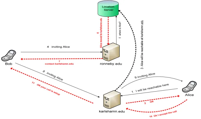
All above SIP Server types are logical functions, so they may reside in one or more physical entities. Typical, SIP Server does include all these function in one machine. Now, to understand how SIP entities works, let us consider the example shown in Figure 1. Bob and Alice have SIP phones working as UAs, in the rest of example we will refer to Bob and Alice as their UAs. Alice at this moment stays geographically in “Karlshamn”, so it registers with the SIP server that serves this area which is “karlshamn.edu”, the registration process means that Alice will be reachable at the domain “karlshamn.edu”, the server “karlshamn.edu” accepts the registration and in turn updates the location server with the new location of Alice. Afterwards, Bob wants to call Alice, so it will send an invitation to its outbound proxy server “ronneby.edu” that consequently seeks the location of Alice using the location server, and when it obtains the location of Alice, it sends a new invitation to Alice using “karlshamn.edu” which does forward the invitation to Alice. After Alice accepts the call, the session now gets setup.
In the previous example we notice that “ronneby.edu” is a proxy and redirect server, where “karlshamn.edu” is a proxy and registrar server.
Figure 1 SIP Entities and How They Work
2.4 SIP Request/Response Massages
SIP is a transactional protocol similar to Hypertext Transfer Protocol (HTTP), so that it is a request/response protocol. In fact, most of SIP semantics and used methods are inherited from HTTP. SIP messages comprise:
2.4.1 Requests
The main request methods defined in RFC 3261 are:
I. INVITE: is the method used to initiate a sessions by UAC. INVITE message’s body
contains description of session, which may use SDP for example or any other description protocol.
II. ACK: is used to acknowledge the last response to the last INVITE method.
III. BYE: is used to terminate a running session.
IV. CANCEL: is used to cancel awaiting request not yet completed, in other words the
V. REGISTER: is used by UA to inform a SIP server with address of which UA wants to be
contacted with.
VI. OPTIONS: is used to query the capabilities of a UA or server, or to find out its
availability.
There are other request methods defined in other RFCs, these are:
PRACK, PUBLISH, INFO, REFER, MESSAGE, UPDATE, NOTIFY and SUBSCRIBE.
2.4.2 Responses
Response codes are categorized in the following classes:
I. 1xx: this class is called Provisional responses. These messages are generated to show
that a call is progressing, and when a UAC receives such a message for an INVITE; it stops retransmission of request.
II. 2xx: this class indicates success of request.
III. 3xx: this class is called redirection. It is used by servers to indicate other locations
where the user may be found.
IV. 4xx: this class indicates a client error. It is generated to specify an error within the
request, so the request should not be retransmitted again without changing the source of error.
V. 5xx: this class stands for a server error. It is generated by a server to point to an error
with it.
VI. 6xx: this class is known as global error. These kinds of responses are generated by a
server to inform UAC that its request is going to fail globally, so retransmission elsewhere does not work.
2.5 SIP Addressing Scheme
SIP addressing is similar to e‐mail; it uses Uniform Resource Identifier (URI) to address its entities. The SIP URI has the following general form[6]:
“sip:user:password@host:port;uri-parameters?headers”
The details of URI are as following:
• ‘user’ indicates the user name. It is optional field except if ‘@’ is present, then it becomes mandatory.
• ‘password’ is the password of the user, this field is not mandatory and not recommended to be present, as the URI is sent in the clear.
• ‘host’ is mandatory field indicating the host. It may use the domain name or IP address. • ‘port’ is an optional element, determines the port number for sending request.
• ‘uri‐parameters’ are optional fields, having effects on the request.
• ‘headers’ are optional fields, specifying which headers to be comprised within the request. All the following examples are valid SIP URIs: sip:amar@bth.se sips:amar@192.168.166.45 sip:amar:mypassword@bth.se;transport=tcp sip:+46762795825@sudan.com;user=phone
2.6 SIP Message Construction
SIP is a text‐based protocol just like HTTP. The context of its messages is clear and readable by humans. The construction of SIP message consists of the following elements: 2.6.1 Request/StatusLine Request‐Line is the first line used in SIP Request, it consists sequentially of a Request Method, Request‐URI and protocol version then ended by CRLF (acronym for Carriage Return/Line Feed, used in computing to indicate a newline after the text). An example of Request‐Line is:INVITE sip:amar@bth.se SIP/2.0
Status‐Line is the first line used in SIP Response, it consists of protocol version followed by status code, then a reason phrase of the code and ended with CRLF. An example of Status‐Line is:
2.6.2 Headers Any SIP message contains some headers following the Request/Status‐Line, some of them are mandatory and others are optional, depending on the method used. The Headers numbers are many; however we will mention some of them which are most important or commonly used: To: determines the targeted recipient of the request. From: specifies the address of the request creator.
Call‐ID: specifies the identity of a certain INVITE or registrations from a specific user. This
identity must be identical for all requests/response within a dialog1.
CSeq: consists of a sequence number and the method used, and works as a mean of
transactions sequencing.
Max‐Forwards: indicates how many hops a request can go across on its route to target. Via: determines the locations a message will pass throughout its way to destination.
Contact: gives the SIP URI should be used in order to contact UA in the consequent request. Content‐Length: with respect to the message size, this header gives how many octets in the
message body, so if the message has no body, it indicates zero
Content‐Type: provides the type of message body.
2.6.3 Message Body
Before the body of a message, there is a mandatory empty line. The message body contains some information such as session description or other information depending on the method used or response code. Some SIP messages may have no body. • In order to clarify the whole picture, the following example demonstrates the structure of a SIP message:
INVITE sip:alice@bth.se SIP/2.0 Via: SIP/2.0/UDP 192.168.55.66:5060 To: Alice<sip:alice@bth.se> From: Bob<bob@tele.com>;tag=1 Call-ID: 1-7876@192.168.55.66 CSeq: 2 INVITE Contact: sip:bob@tele.com Content-Type:application/sdp Content-Length:143 v=0 o=user1 53655765 2353687637 IN IP4 192.168.55.66 s=Phone Call c=IN IP4 192.168.55.66 t=0 0 m=audio 6000 RTP/AVP 0 a=rtpmap:0 PCMU/8000
2.7 SIP Related Protocols
As SIP is a signaling protocol used for creating multimedia sessions; it has some other protocols where commonly used with, these protocols are: 2.7.1 Session Description Protocol “SDP”When initiating or modifying a session, SIP does need some means of session description so that the participating entities would be able to negotiate and agree on the format and type of media. SDP is commonly used for that purpose, however SIP and SDP are independent. Therefore, any method for session description can be used instead of SDP, for instance Extensible Markup Language (XML) or any means of negotiation protocol that end entities are able to understand. 2.7.2 Session Announcement Protocol “SAP” When SIP is used to initiate a Multicast sessions such as video conferences, SAP is commonly used to broadcast the session description for the participated parties. 2.7.3 Realtime Transport Protocol “RTP”
RTP is an application layer protocol, used for transport of real‐time media such as audio and video over IP networks. SIP and RTP are usually used in conjunction, so that RTP used for transporting of data and SIP for controlling it. The most common application nowadays for RTP is the VoIP.
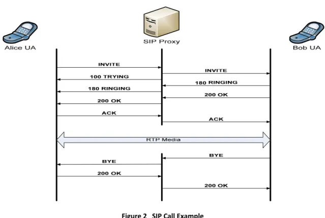
2.8 SIP Call Example
The following example shows a SIP call between two UAs using a SIP proxy in‐between as shown in Figure 2.
Figure 2 SIP Call Example
Bob wants to make a call to Alice using his SIP phone as a UA, the flow of call will go like following:
Bob sends “INVITE” to Alice through the proxy which in turn forwards the message to Alice, then sends back Bob “100 Trying” response so that Bob UA knows its request is now under process, after Alice receives Bob’s invitation; her SIP phone start ringing generating “180 Ringing” response which is forwarded back to Bob through the proxy and Bob now can here the ring back tone. When Alice picks up her phone a “200 Ok” response is sent from Alice UA to Bob’s, and when Bob receives the message the call now is setup and they can talk to each other. At the end of their call any one can hang up triggering a “BYE” request and the other UA responds with “200 Ok” when receiving the “BYE” request.
Chapter 3: System Design
This chapter discusses our system design, it shows which objects we want to measure, and then it describes all scenarios used in our experiments and all models as well.
3.1 Objects of Measurements
Our point of attention in experiments is to measure SIP session setup delay. This delay as shown in Figure 3 consists of the following periods [7]: I. Post‐Dial Delay: The time interval since calling terminal initiates the call until it gets indication message that call has been received. In SIP call, it is the time interval between UAC sends INVITE message until it receives 180 RINGING message. II. Ringing Delay
In SIP call, it is the time interval between UAC receives 180 RINGING messages until getting back 200 OK message. The ringing period is an object varies depending on humans’ behavior. In this research, we are not interested to model it. III. Answer‐Signal Delay: The time interval since the called terminal being connected to the call until the calling terminal being notified with this. In SIP call, it is the time interval between UAS sends 200 OK message until it gets back ACK message.
3.2 Scenarios
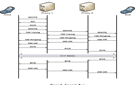
In order to implement SIP call scenarios, we have chosen six scenarios adapted from RFC 3665 “Session Initiation Protocol (SIP) Basic Call Flow Examples”[8], these scenarios are some simple examples of successful SIP calls with different circumstances. These scenarios are: 3.2.1 Scenario One This scenario is the simplest one, there are only two UAs talking to each other directly. Alice’s device works as UAC and Bob’s as UAS as shown in Figure 4 Figure 4 Scenario One 3.2.2 Scenario Two In this scenario, Alice (UAC) calls Bob (UAS) through two SIP proxies in the middle, Alice Sends INVITE message to Proxy 1 which is the default proxy for Alice, the INVITE message does not contain the authorization credentials so that Proxy 1 challenges Alice for credentials with 407 response which is “Proxy Authorization Required”, Alice responds with sending a new INVITE with its right credentials and Proxy 1 forward the message, and then the call gets established.
Figure 5 Scenario Two
3.2.3 Scenario Three
This scenario is the same like previous one except that here there are two Proxy Authentication required, so that Proxy 1 will do one challenge for credentials (like in scenario 2), and after Alice sends the second INVITE, Proxy 2 also makes another challenge with 407 response, and then Alice sends the third INVITE with the right credentials for both Proxy 1 and Proxy 2, as Alice does have the credentials for both Proxies.
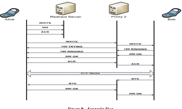
3.2.4 Scenario Four In this Scenario, Alice is configured to use Proxy 1 as the first choice (Primary) and Proxy 2 as a second choice (secondary). Alice sends an INVITE message to Proxy 1 which is unresponsive at this moment for some reason, and after resending the INVITE seven times, the timeout takes place. Then, Alice sends a new INVITE over Proxy 2, and then the call setup goes on as normal. Figure 7 Scenario Four 3.2.5 Scenario Five In this Scenario, Alice calls Bob using a Redirect and Proxy Servers in‐between, Alice sends an INVITE message to the Redirect Server which in turn responds by 302 response “Moved Temporarily” which contains the SIP address of Bob in its Contact header, then Alice sends another INVITE over Proxy 2, and the call proceeds normally.
Figure 8 Scenario Five
3.2.6 Scenario Six
In this scenario, Alice sends an INVITE to Bob using one Proxy server in the middle, and the call gets established as normal. After that and during the session, Bob changes its IP address, so that it sends a new INVITE to Alice showing its new address, and the session is proceeded after the three‐way handshake (INVITE‐200 OK‐ ACK). Our interest in this research is the delay which happens at the three‐way handshake as this delay is very important to study, especially when using SIP as the mobility management protocol in the handover between different networks.
3.3 Design Models
3.3.1 Actual situation
In this research, our main target is to model the SIP session setup delay, and the scenarios above are implemented for doing the modeling. However, to do this modeling, we have to study how SIP call looks like over the Internet. Figure 10 shows a typical SIP call over the Internet. Alice and Bob are User Agents, and there are two SIP Servers each one lies geographically near from a User Agent and the Internet is between them, this is a typical situation in reality.
When Alice Initiates a call to Bob, any SIP message traversing between them does experience some delay. We have to consider that any SIP message is encapsulated eventually into an IP datagram.
To analyze this delay, we refer to Figure 10 below; the delay is divided into three stages:
• Delay 1: is the delay a packet experiences while traversing between SIP UA and SIP Server. This delay supposed to be minor since UA and Server lie near from each other as we mentioned before. • Delay 2: This is the delay a packet experiences while traversing between the SIP Servers. Actually, this is the major delay, which is the Internet delay. • Delay 3: is the same like delay 1. Figure 10 Typical SIP Call Over The Internet
3.3.2 Modeling
When doing modeling for a SIP call, we have to consider the delays mentioned above. Moreover, because we are modeling SIP over UDP, we are interested in the One‐Way Transmit Time (OWTT) for the IP packet instead of Round‐Trip Time (RTT). For the sake of implementing our models we are going to assume:
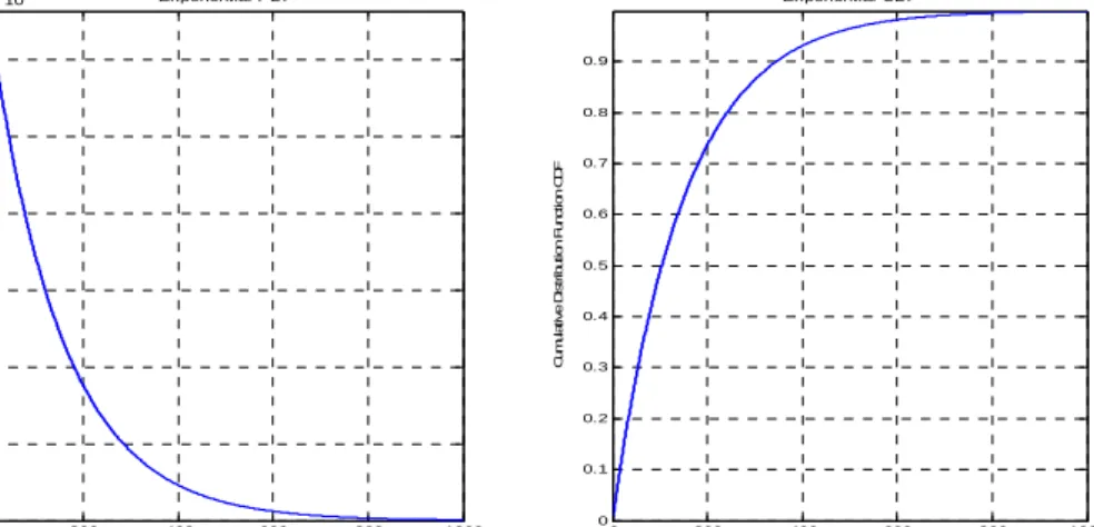
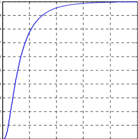
I. Delay 1 and 3 model: These delays do not have high values because the entities are physically close to each other. In [9] some measurements done between two entities to determine the One‐Way Internet Packet Delay, there were three routers between entities, and the measurements gave mean value ranging between 2 to 16 milliseconds. In our model we are going to assume a random OWTT with the mean of 10 milliseconds following Exponential Statistical Distribution. As these delays are minor relative to Delay 2, Exponential Distribution would be the best to model these delays.
II. Delay 2: This is the main delay that any packet does experience. Many researches studied Internet end‐to‐end performance. However, it is very difficult to propose specific model for this delay. In this research, we are going to propose three models to emulate Internet end‐to‐end delay. We assume that this delay has a random OWTT with mean of 150 millisecond following three statistical distributions: Exponential, Lognormal and Pareto Distributions. We are going to discuss the implementation of the test bed and compare the results of all models in the next chapters. In the next section we detail these three models.
Exponential Model
To demonstrate Exponential Distribution, the equations below shows the Probability Density ) a umulative Distribution Function (CDF) respectively.
Function (PDF nd the C
‐‐‐‐‐‐‐‐‐‐‐‐‐‐‐‐‐‐‐‐‐‐‐‐‐‐‐‐‐‐‐‐‐‐ Equation 1 (Exponential PDF) ‐‐
‐‐‐‐‐‐‐‐‐‐‐‐‐‐‐‐‐‐‐‐‐‐‐‐‐‐‐‐‐‐‐‐‐‐ Equation 2 (Exponential CDF)
The mean nda variance are given by:
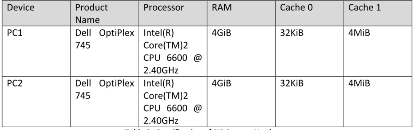
Figure 11 displays the Exponential Distribution Functions, both PDF and CDF using the mean of 150 millisecond. 0 200 400 600 800 1000 0 1 2 3 4 5 6 x 10⁻³ x(ms) P ro b a b ility D ens it y F unc ti o n P D F Exponential PDF 0 200 400 600 800 1000 0 0.1 0.2 0.3 0.4 0.5 0.6 0.7 0.8 0.9 x(ms) C um u la tiv e D is tr ibu ti on Func ti on C D F Exponential CDF Figure 11 Exponential Distribution Function
Lognormal Model
Lognormal Distribution has the property that its logarithm result in Normal Distribution, the e uq atio s b o shn el w ows the PDF and CDF re spectively
√ / , 0 ‐‐‐‐‐‐‐‐‐‐‐‐‐‐‐‐‐‐‐‐‐‐‐‐‐‐‐‐‐ Equation 4 (Lognormal PDF) , √ ‐‐‐‐‐‐‐‐‐‐‐‐‐‐‐‐‐‐‐‐‐‐‐‐‐‐‐‐‐ Equation 5 (Lognormal CDF)
The mean and ar av i nce are given by
⁄
‐‐‐‐‐‐‐‐‐‐‐‐‐‐‐‐‐‐‐‐‐‐‐‐‐‐‐‐‐‐ Equation 6 (Mean and Variance)
μ
0 200 400 600 800 1000 0 1 2 3 4 5 6 7x 10 -3 x(ms) P ro b a b ility D ens it y F unc ti o n P D F Lognormal PDF 0 200 400 600 800 1000 0 0.1 0.2 0.3 0.4 0.5 0.6 0.7 0.8 0.9 1 x(ms) C um u lat iv e D is tr ibu ti on Func ti on C D F Lognormal CDF Figure 12 Lognormal Distribution Function
Pareto Model
P eto Disar tribution is often used to model Internet traffic. Its PDF and CDF are shown below. ‐‐‐‐‐‐‐‐‐‐‐‐‐‐‐‐‐‐‐‐‐‐‐‐‐‐‐‐‐‐‐‐ Equation 7 (Pareto PDF) ‐‐‐‐‐‐‐‐‐‐‐‐‐‐‐‐‐‐‐‐‐‐‐‐‐‐‐‐‐‐‐‐ Equation 8 (Pareto CDF) WhereThe mean and variance are given by
‐‐‐‐‐‐‐‐‐‐‐‐‐‐‐‐‐‐‐‐‐‐‐‐‐‐‐‐‐ Equation 9 (Mean and Variance)
Where a is the minimum value that x can take, and b is a positive factor.
Figure 13 displays Pareto PDF using the mean of 150 millisecond, where a and b equal 3 and 100 millisecond respectively.
0 200 400 600 800 1000 0 0.005 0.01 0.015 0.02 0.025 0.03 x(ms) P ro b a b ility D ens it y F unc ti o n P D F Pareto PDF 0 200 400 600 800 1000 0 0.1 0.2 0.3 0.4 0.5 0.6 0.7 0.8 0.9 x(ms) C um u lat iv e D is tr ibu ti on Func ti on C D F Pareto CDF Figure 13 Pareto Distribution Function
Chapter 4: Experimental Setup
This chapter presents how we did the setup for our experiments, so that we introduce our test bed hardware and software components and how we have built it.4.1 Hardware Components
• Two Desktop PCs working as SIP User Agents, and their specifications are the following: Device Product NameProcessor RAM Cache 0 Cache 1
PC1 Dell OptiPlex
GX260
Intel(R) Pentium(R) 4 CPU 2.00GHz
1GiB 8KiB 512KiB
PC2 Dell OptiPlex
GX260
Intel(R) Pentium(R) 4 CPU 2.00GHz
1GiB 8KiB 512KiB
Table 1 Specification of SIP User Agents Hardware • Two Desktop PCs working as SIP Servers and their specifications are the following: Device Product Name
Processor RAM Cache 0 Cache 1
PC1 Dell OptiPlex 745 Intel(R) Core(TM)2 CPU 6600 @ 2.40GHz
4GiB 32KiB 4MiB
PC2 Dell OptiPlex 745 Intel(R) Core(TM)2 CPU 6600 @ 2.40GHz
4GiB 32KiB 4MiB
Table 2 Specification of SIP Servers Hardware
• One switch : NETGEAR FS608 8‐Port 10/100 Fast Ethernet
4.2 Software Components
The software used in the test bed is the following: 4.2.1 Operating System In all PCs we used KUBUNTU Hardy 8.4 as an operating system. It has a Graphical User interface, so it is user friendly and simple to use. 4.2.2 SIPp version 3.1It is an open source SIP tool, compliant to RFC 3261. It is very efficient and flexible tool. By using it, user can generate traffic and build User Agents both client and server. SIPp has embedded call scenarios, and has the capability to run input scenarios written in XML files. It has a lot of feature, for example it does support different transport protocols like UDP, TCP and TLS. In addition it has other features like its ability to send RTP media and many other features as well [10]. In our test bed we used SIPp to build User Agents in all scenarios. 4.2.3 SIP Express Router (SER) version 0.9.6 SER is an open source SIP server, compliant to RFC 3261. It is very powerful server that can be configured as SIP proxy, registrar and/or redirect server. SER is very flexible, so that it behaves depending on user’s input configuration file [11].
4.3 Building the test bed
In this section, we detail how we built the test bed, so that we present the whole hardware and software installation procedures. 4.3.1 Hardware InstallationIn the lab, we used hardware components mentioned above to build the test bed shown in Figure 14. Two of the PCs used as SIP Servers and the other two used as SIP User Agents, all these components are connected to the switch by straight cables to their Network Cards. The figure also demonstrates Delay 1,2 and 3 which are the delays shown before in Figure 10, using the software we are going to inject these delays to emulate the delays happen in reality.
Figure 14 Test Bed Hardware Installation 4.3.2 Software Installation In this section we present the main installation procedure for all softwares mentioned above. After completing all installations, the test bed is ready for running all scenarios. However, each scenario has its own XML script and configuration file used in SIPp and SER respectively2. I. KUBUNTU Hardy 8.4
It is an open source operating system available for free in the web, where any one can download and burn in a CD, or even order a CD for free. The installation is very easy, just to put the CD in its drive, reboot the PC then follow the wizard. We did install it in all PCs we are using. II. SIPp version 3.1 It is open source software, so that user can download it for free from the web. The installation procedure is [10]:
Using a web browser, go to http://sipp.sourceforge.net/ , then go to Downloads and download version 3.1
In order to compile SIPp, we have to install some libraries as prerequisites, to do that open a terminal and execute the following:
$ sudo apt-get install ncurses-dev
$ sudo apt-get install openssl $ sudo apt-get install gsl-bin
$ sudo apt-get install libnet1
$ sudo apt-get install libpcap-dev
Now we can install SIPp by executing the following through a terminal: $ sudo su # tar xzfv sip-yyy.tar.gz3 # make pcapplay_ossl After doing this, the installation runs smoothly. III. SER verison 0.9.6 Is open source software available for free in the web, to install it we do the following [11]: Download it from http://www.iptel.org/download
We need database to save SIP addresses and domains, so that we are going to use MYSQL database, just we open a terminal and execute:
$ sudo apt-get install mysql-server
To compile SER, we have to install some prerequisites as follows:
$ sudo apt-get install bison flex sed libexpt1 libpq
then:
$ sudo su
# make all include_modules="mysql”
# make install
Now the installation runs.
Then to create the database of SER we run the command:
# ser_msql.sh create
The installation now is complete.
4.3.3 Synchronization
With the aim of doing measurement that depends on more than one party, we need to synchronize the clocks of participating entities. In all our experiments, we are taking the timestamps of SIP Requests/Responses in both UAC and UAS, to calculate session setup delays. Calculating Post‐Dial and Answer‐Signal Delays does not require synchronizing entities, as it depends only on SIP Requests/Responses in one side. However, synchronizing UAC and UAS is a requisite in Scenario‐Six for calculating Setup‐Delay.
In our test bed, we have used NTP Servers to synchronize the entities, and one of these servers resides at Blekinge Institute of Technology (BTH), where these experiments are done.
Chapter 5: Results and Analysis
In this chapter we present the results and analysis of our experiments, we begin with demonstrating the results of different models used, and then we show the performance of each model and compare them to each other.
5.1 Results of models
In our measurements, for each scenario we run the three models: Exponential, Lognormal and Pareto Models to get SIP session setup delay. For each experiment we run 10 batches, each batch consist of 5500 SIP call.
We logged the timestamps for each SIP request/response in both entities UAC and UAS. Then using the excel sheets we calculated the Post‐Dial Delay and Answer‐Signal Delay for all scenarios except Scenario‐Six. In Scenario‐Six, we are interested in calculating the setup‐delay for the Re‐INVITE as we mentioned before in chapter 3. We aggregated the results of each scenario and calculated the statistical properties’ elements. Table 3 shows the statistical elements for Post‐Dial Delay for all scenarios except Scenario‐Six. Scenario Model mean (sec) stdev MAX (sec) MIN (sec) CORREL lag1 CORREL lag2 95% confidence interval 1 Exponential 0.3046 0.2140 2.1681 0.0078 0.0146 ‐0.0018 1.8761E‐03 1 Lognormal 0.3055 0.1882 2.6682 0.0315 0.0002 ‐0.0039 1.6498E‐03 1 Pareto 0.3054 0.1319 4.9598 0.2043 0.0008 0.0030 1.1561E‐03 2 Exponential 0.3686 0.2293 9.8106 0.0312 0.0033 0.0056 2.0101E‐03 2 Lognormal 0.3668 0.1908 10.0493 0.0629 ‐0.0023 ‐0.0017 1.6724E‐03 2 Pareto 0.3694 0.1580 10.1875 0.2203 0.0027 ‐0.0015 1.3849E‐03 3 Exponential 0.7078 0.3246 10.8541 0.0803 ‐0.0019 ‐0.0021 2.8455E‐03 3 Lognormal 0.7065 0.2759 10.2088 0.1971 ‐0.0041 0.0095 2.4184E‐03 3 Pareto 0.7077 0.1971 9.8631 0.4599 ‐0.0020 0.0003 1.7280E‐03 4 Exponential 32.6880 0.3040 42.3293 32.1002 ‐0.0024 0.0060 2.6644E‐03 4 Lognormal 32.6829 0.2659 41.9371 32.1664 0.0037 ‐0.0020 2.3311E‐03 4 Pareto 32.6849 0.2023 42.2847 32.4557 0.0017 ‐0.0001 1.7731E‐03 5 Exponential 0.3688 0.2226 10.4500 0.0363 0.0053 0.0000 1.9510E‐03 5 Lognormal 0.3683 0.2121 10.1761 0.0640 0.0072 0.0018 1.8587E‐03 5 Pareto 0.3680 0.1434 6.8035 0.2217 0.0004 0.0004 1.2567E‐03 Table 3 Post‐Dial Delay Results
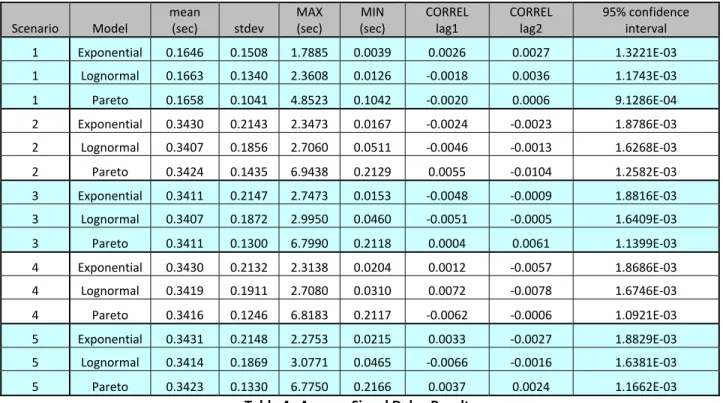
Table 4 shows the statistical elements for Answer‐Signal Delay for all scenarios except Scenario‐ Six. Scenario Model mean (sec) stdev MAX (sec) MIN (sec) CORREL lag1 CORREL lag2 95% confidence interval 1 Exponential 0.1646 0.1508 1.7885 0.0039 0.0026 0.0027 1.3221E‐03 1 Lognormal 0.1663 0.1340 2.3608 0.0126 ‐0.0018 0.0036 1.1743E‐03 1 Pareto 0.1658 0.1041 4.8523 0.1042 ‐0.0020 0.0006 9.1286E‐04 2 Exponential 0.3430 0.2143 2.3473 0.0167 ‐0.0024 ‐0.0023 1.8786E‐03 2 Lognormal 0.3407 0.1856 2.7060 0.0511 ‐0.0046 ‐0.0013 1.6268E‐03 2 Pareto 0.3424 0.1435 6.9438 0.2129 0.0055 ‐0.0104 1.2582E‐03 3 Exponential 0.3411 0.2147 2.7473 0.0153 ‐0.0048 ‐0.0009 1.8816E‐03 3 Lognormal 0.3407 0.1872 2.9950 0.0460 ‐0.0051 ‐0.0005 1.6409E‐03 3 Pareto 0.3411 0.1300 6.7990 0.2118 0.0004 0.0061 1.1399E‐03 4 Exponential 0.3430 0.2132 2.3138 0.0204 0.0012 ‐0.0057 1.8686E‐03 4 Lognormal 0.3419 0.1911 2.7080 0.0310 0.0072 ‐0.0078 1.6746E‐03 4 Pareto 0.3416 0.1246 6.8183 0.2117 ‐0.0062 ‐0.0006 1.0921E‐03 5 Exponential 0.3431 0.2148 2.2753 0.0215 0.0033 ‐0.0027 1.8829E‐03 5 Lognormal 0.3414 0.1869 3.0771 0.0465 ‐0.0066 ‐0.0016 1.6381E‐03 5 Pareto 0.3423 0.1330 6.7750 0.2166 0.0037 0.0024 1.1662E‐03 Table 4 Answer‐Signal Delay Results Table 5 shows statistical elements for Setup‐Delay in Scenario‐Six Scenario Model mean (sec) stdev MAX (sec) MIN (sec) CORREL lag1 CORREL lag2 95% confidence interval 6 Exponential 0.4541 0.2158 2.9973 0.0137 0.0025 0.0082 1.8915E‐03 6 Lognormal 0.4574 0.1899 2.7418 0.1454 ‐0.0014 ‐0.0114 1.6644E‐03 6 Pareto 0.4613 0.1524 5.3304 0.3258 ‐0.0041 0.0026 1.3361E‐03 Table 5 Scenario‐Six Setup Delay
Using the results we got through experiments, we used MATLAB to estimate and plot the Distribution Functions both PDF and CDF for each scenario.
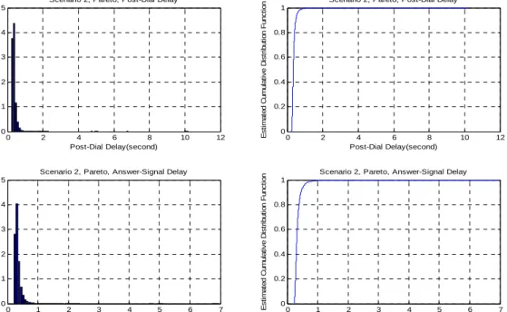
In order to analyze the performance of used models, we will investigate the results of Scenario‐ Two as an example4, so that we can assess the performance of these models.
Figure 15 to Figure 17 demonstrate the results of Exponential, Lognormal and Pareto models respectively. They show the estimated PDF and CDF for both Post‐Dial Delay and Answer‐Signal Delay. 0 2 4 6 8 10 0 0.05 0.1 0.15 0.2 0.25 Post-Dial Delay(second) E s ti ma te d P ro b a b ilit y D e n s it y F u n c ti o n
Scenario 2, Exponential, Post-Dial Delay
0 2 4 6 8 10 0 0.2 0.4 0.6 0.8 1 Post-Dial Delay(second) E s ti m at ed C um ul at iv e D is tr ibut ion F unc ti on
Scenario 2, Exponential, Post-Dial Delay
0 0.5 1 1.5 2 2.5 0 0.01 0.02 0.03 0.04 0.05 0.06 Answer-Signal Delay(second) E s ti m at ed P robabi lit y D ens it y F unc ti on
Scenario 2, Exponential, Answer-Signal Delay
0 0.5 1 1.5 2 2.5 0 0.2 0.4 0.6 0.8 1 Answer-Signal Delay(second) E s ti m at ed C um ul at iv e D is tr ibut ion F unc ti on
Scenario 2, Exponential, Answer-Signal Delay
. Figure 15 Estimated PDF and CDF for Exponential Model 0 2 4 6 8 10 12 0 0.05 0.1 0.15 0.2 0.25 0.3 0.35 Post-Dial Delay(second) Es ti m a te d P ro b a b ilit y D e n s it y F u n c ti o n
Scenario 2, Lognormal, Post-Dial Delay
0 2 4 6 8 10 12 0 0.2 0.4 0.6 0.8 1 Post-Dial Delay(second) Es ti m at e d C um u lat iv e D is tr ib ut ion F unc ti o
n Scenario 2, Lognormal, Post-Dial Delay
0 0.5 1 1.5 2 2.5 3 0 0.02 0.04 0.06 0.08 0.1 Answer-Signal Delay(second) Es ti m a te d P ro b a b ilit y D e n s it y F u n c ti o n
Scenario 2, Lognormal, Answer-Signal Delay
0 0.5 1 1.5 2 2.5 3 0 0.2 0.4 0.6 0.8 1 Answer-Signal Delay(second) Es ti m at ed C um ul at iv e D is tr ib u ti o n Fu nc ti on
Scenario 2, Lognormal, Answer-Signal Delay
0 2 4 6 8 10 12 0 0.1 0.2 0.3 0.4 0.5 Post-Dial Delay(second) E s tim a te d P ro b a b ilit y D e n s it y F u n c tio n
Scenario 2, Pareto, Post-Dial Delay
0 2 4 6 8 10 12 0 0.2 0.4 0.6 0.8 1 Post-Dial Delay(second) E s ti m at e d C u m u lat iv e D is tr ib ut ion F u nc ti on
Scenario 2, Pareto, Post-Dial Delay
0 1 2 3 4 5 6 7 0 0.1 0.2 0.3 0.4 0.5 Answer-Signal Delay(second) E s ti m a te d P ro b a b ility D e n s ity F u n c ti o n
Scenario 2, Pareto, Answer-Signal Delay
0 1 2 3 4 5 6 7 0 0.2 0.4 0.6 0.8 1 Answer-Signal Delay(second) E s ti m at e d C u m u lat iv e D is tr ibut ion F u nc ti on
Scenario 2, Pareto, Answer-Signal Delay
Figure 17 Estimated PDF and CDF for Pareto Model
5.2 Analysis
In order to assess the performance of the three models, we want to see which distributions the Post‐Dial and Answer‐Signal Delays are following. Referring to the figures resulted above, we observe that the closest distributions to them are Rayleigh and Lognormal Distributions. Using the resulted mean and standard deviation we plotted the corresponding distribution functions of Rayleigh and Lognormal Distribution, so that we can compare. 5.2.1 Rayleigh Distribution One of the well‐known distribution functions is known as Rayleigh Distribution which has the distribution function PDF and CDF given by: ⁄ ‐‐‐‐‐‐‐‐‐‐‐‐‐‐‐‐‐‐‐‐‐‐‐‐‐‐‐‐‐ Equation 10 (Rayleigh PDF) ⁄ ‐‐‐‐‐‐‐‐‐‐‐‐‐‐‐‐‐‐‐‐‐‐‐‐‐‐‐‐‐‐ Equation 11 (Rayleigh CDF) The mean and variance a e given by r ‐‐‐‐‐‐‐‐‐‐‐‐‐‐‐‐‐‐‐‐‐‐‐‐‐‐‐‐‐‐‐ Equation 12 (Mean and Variance)
Referring to Table 3 and Table 4, for Scenario‐Two:
The mean values for Post‐Dial and Answer‐Signal delays using Exponential model equal to 0.3686 and 0.343 seconds respectively, which more or less are the same for the two other models
With the same mean values of (0.3686 and 0.343 seconds), we have plotted Rayleigh Distribution Function using MATLAB as shown in Figure 18 and Figure 19. 0 500 1000 1500 2000 0 0.5 1 1.5 2 2.5x 10 -3 x(ms) Pr obabi li ty D e ns it y Func ti on PD F Rayleigh PDF 0 500 1000 1500 2000 0 0.1 0.2 0.3 0.4 0.5 0.6 0.7 0.8 0.9 1 x(ms) C um ul at iv e D is tr ibut ion Fun c ti on C D F Rayleigh CDF Figure 18 Corresponding Post‐Dial Delay Rayleigh Distribution Function 0 500 1000 1500 2000 0 0.5 1 1.5 2 2.5x 10 -3 x(ms) P robab il it y D ens it y F unc ti on P D F Rayleigh PDF 0 500 1000 1500 2000 0 0.1 0.2 0.3 0.4 0.5 0.6 0.7 0.8 0.9 1 x(ms) C um ul at iv e D is tr ib u tio n F u n c tio n C D F Rayleigh CDF Figure 19 Corresponding Answer‐Signal Delay Rayleigh Distribution Function
5.2.2 Lognormal Distribution
Now, with the same mean values (0.3686 and 0.343 seconds), we have plotted Lognormal Distribution Functions PDF and CDF as shown in Figure 20 and Figure 21. 0 500 1000 1500 2000 0 0.5 1 1.5 2 2.5 3x 10 -3 x(ms) P ro b a b ility D ens it y F unc ti o n P D F Lognormal PDF 0 500 1000 1500 2000 0 0.1 0.2 0.3 0.4 0.5 0.6 0.7 0.8 0.9 1 x(ms) C um ul a ti v e D is tr ibu ti on Func ti on C D F Lognormal CDF Figure 20 Corresponding Post‐Dial Delay Lognormal Distribution Function 0 500 1000 1500 2000 0 0.5 1 1.5 2 2.5 3x 10 -3 x(ms) P ro b a b ilit y D en s it y F unc ti on P D F Lognormal PDF 0 500 1000 1500 2000 0 0.1 0.2 0.3 0.4 0.5 0.6 0.7 0.8 0.9 1 x(ms) C um ul a ti v e D is tr ibut ion Func ti on C D F Lognormal CDF Figure 21 Corresponding Answer‐Signal Delay Lognormal Distribution Function
5.2.3 Discussion
From our experiments results obtained, and in order to produce models for SIP session setup delays, we point out the following:
• In all our experiments, we have injected random delays for any sent SIP request/response, as we mentioned before, with different distribution functions, which means that delays’ values are uncorrelated.
• Referring to the tables of results above for all used models, we can see that the values obtained for Post‐Dial and Answer‐Signal Delays have very little correlations for both Lag1 and Lag2. Since many SIP requests/responses are participating to create Post‐Dial and Answer‐Signal Delays, having uncorrelated values for these delays is anticipated. • In all used models and for all scenarios, we can see that the mean values of Post‐Dial
and Answer‐Signal Delays are almost the same for all models, since the injected random delays have the same mean values for all models.
• Throughout all the tables above, regarding minimum and maximum values for both Post‐Dial and Answer‐Signal Delays, we observe that Pareto model usually has the trend to produce the highest values for these delays, and Exponential model to produce the lowest. This happens as a result of that Pareto Distribution Function has a heavier tail than Lognormal and Exponential Distribution Functions.
• If we compare the PDF and CDF illustrated in Figure 15, Figure 16 and Figure 17 obtained by Exponential, Lognormal and Pareto respectively, with Figure 18 to Figure 21 created by Rayleigh and Lognormal Distribution Functions with the same mean values; we notice:
I. Exponential and Lognormal models produce Post‐Dial and Answer‐Signal Delays that seem to be following a Distribution Function of somewhere between Rayleigh and Lognormal Distributions.
II. For Pareto model, it is not easy to judge that it does follow a specific distribution, however its PDF and CDF is near from Lognormal Distribution Function illustrated in Figure 20 and Figure 21.
• Observing all resulted figures for remaining scenarios5, we can see that their PDF and
CDF have almost the same behavior of scenario‐Two analyzed above.
• Since our experiments took into consideration various SIP call scenarios, and the results gave more or less the same performance with respect to distribution functions; we propose using Lognormal and Rayleigh distribution functions to model SIP session setup delays independently of the architecture of SIP elements participating in the session. 5.2.4 Proposed Models for SIP Session Setup Delays With the aim of elaborating the added value of this effort, we make a review for the previous work addressing the SIP session setup delay, and then we present what is accomplished here. In [2] the authors addressed the session setup delay in both SIP and H.323 running over UDP and TCP respectively. Using Internet delays taken from [12], they made simulation for calls setup using different scenarios of both H.323 and SIP. The results showed that the performance of SIP over UDP is better than H.323 over TCP with respect to the setup delay.
Also in [3] SIP setup delays were investigated for video sessions, the study was focused on the performance over 3G networks. Their experiments were carried out using 3G network emulator. According to their results, they proved that the delays incurred by session setup are acceptable in 3G networks. In [1] session setup performance was studied for both SIP and H.323, and the results showed that the delays caused by SIP are lesser than those of H.323. Moreover, the setup delays of SIP over UDP were found to be 30% less than those over TCP. Additionally, the experiments proved that session setup delays can be more decreased when using retransmission protocols such as RLC.
In all previous researches SIP session setup delays were investigated with the purpose of determining the amount of delay, how these delays might affect interconnection with PSTN, or comparing the performance of SIP with its competitors. This effort also does address the setup delays; however the concern here is to create some models for these delays rather than just presenting the values obtained by simulations.
As IP datagram delay over the Internet is the major issue to consider when trying to create such models, we have introduced three models to be used for emulating the Internet delays, and based on the results of experiments done for each model; we propose two models to be used for SIP session setup delays, taking into consideration the used scenario in order to determine the mean and standard deviation, and these are:
I. Lognormal Model
This model can be used to model setup delays regardless of which distribution function the Internet delay is following, as we considered three different distribution functions for the former delay.
II. Rayleigh Model
If we assume that the Internet delay is following Lognormal or Exponential distribution function, then Rayleigh distribution can also model SIP session setup delays.
Chapter 6: Conclusion
Throughout this document, we have addressed the delay caused by initiating the SIP session. We have presented general features of SIP and how it works, then we went through the details of our design and the scenarios used to do the experiments. After that, we detailed the procedures of building the test bed. Then, we showed the results of all experiments and we have analyzed and evaluated them.
Studying the delays incurred by creating session using SIP is quite interesting as this area of research has not acquired a lot of consideration.
In this context, our aim was to do some modeling, and in order to create valid models for SIP session setup delay components, we have used different distribution functions, so that we could compare the performance of each model.
In our test bed, we have injected random delays for the transmitted SIP message in order to simulate the delays experienced by any message in reality. Our assumption that messages do experience random delays while crossing the same routes through the Internet is not completely true, as there would be always some correlation between these delays in such a situation over the Internet. After we examined the resulted delays of our three models, there was some similarity between them with regard to the distribution functions of the results, which may prove that the resulted delays of session setup delay components do not totally depend on which distribution function the Internet delays is following. SIP by its nature, does support the user mobility and also can be used to support terminal and session mobility [13]. In the next generation networks, mobile nodes supposed to have a seamless communication, so that a vertical handover between heterogeneous networks is required. SIP and Mobile IP (MIP) are dedicated to be used as mobility management protocols in such a handover. This area of research is quite interesting for SIP as MIP still does have some limitations.
AppendixA: Abbreviations
CDF: Cumulative Distribution Function CRLF: Carriage Return/Line Feed GSM: Global System for Mobile communication HTTP: Hypertext Transfer Protocol IETF: Internet Engineering Task Force IP: Internet Protocol IPTV: Internet Protocol Television LAN: Local Area Network MIP: Mobile IP OWTT: One‐Way Transmit Time PC: Personal Computer PDF: Probability Density Function PSTN: Public Switched Telephone Network RLC: Radio Link Protocol RTP: Real‐time Transport Protocol RTT: Round‐Trip Time SAP: Session Announcement Protocol SCIP: Simple Conference Invitation Protocol SCTP: Stream Control Transmission Protocol SDP: Session Description Protocol SIP: Session Initiation Protocol SIPv1: Session Invitation Protocol version 1 SS7: Signaling System Number 7 TCP: Transport Control Protocol TLS: Transport Layer Security UA: User AgentUAS: User Agent Server UDP: User Datagram Protocol URI: Uniform Resource Identifier XML: Extensible Markup Language