Design of High Performance Flanges and its Influence on Manufacturing Costs, Structural Performance and Weight

(1)

Design of high performance flanges and its

influence on manufacturing costs, structural

performance and weight

Joaquin Alcocer Bonifaz

Master of Science Thesis TRITA-ITM-EX 2019:70 KTH Industrial Engineering and Management

Machine Design SE-100 44 STOCKHOLM

(2)

(3)

Examensarbete TRITA–ITM–EX 2019:70 Konstruktion av högpresterande flänsförbands inverkan på tillverkningskostnader, prestanda och vikt

Joaquin Alcocer Bonifaz

Godkänt

2019-03-24 Examinator _{Ulf Sellgren} Handledare _{Ellen Bergseth}

Uppdragsgivare

GKN Aerospace

Kontaktperson

Per Widström

Sammanfattning

Syftet för detta projekt är att undersöka tillverkningskostnaden, med tonvikt på bearbetning av högpresterande flänsar för turbinapplikationer (TRS), samt dess relation till strukturella prestanda och vikt. Traditionella kostnadsmodelleringstekniker kombineras med det icke-konventionella tillverkningskomplexitetsindexet och används som kostnadsindikator. En tvärvetenskaplig studie genomförs med hjälp av ANSYS Workbench i form av dator simulerade experiment för att undersöka flänsavvägningar. En slutsats av studien är att multidisciplinära modeller av kostnad, prestanda och vikt saknade robusthet för att kunna dra djupgående slutsatser om prestandan för en flänsdesign. Tillverkningskomplexitetsindexet visar dock, efter partiell validering med erfarna ingenjörer, lovande resultat och kan vara framgångsrikt ett sätt att uppskatta den slutliga bearbetningskostnaden för flänsar.

Nyckelord: tillverkningskostnadsmodellering, datorsimulerade experiment,

(4)

(5)

Master of Science Thesis TRITA–ITM–EX 2019:70 Design of high performance flanges and its influence on manufacturing costs, structural performance and weight

Joaquin Alcocer Bonifaz

Approved

2019-03-24 Examiner _{Ulf Sellgren} Supervisor _{Ellen Bergseth}

Commissioner

GKN Aerospace

Contact person

Per Widström

Abstract

This project attempts to research the manufacturing cost, with an emphasis on machining, of high performance flanges for Turbine Rear Structure (TRS) applications, as well as the tradeoffs with structural performance and weight. A combination of traditional cost modelling techniques from the literature, as well as, the non-conventional manufacturing complexity index, as cost indicator are implemented. A multidisciplinary study is carried out with the aid of ANSYS Workbench in the form of computer simulated experiments to investigate tradeoffs in flanges. It is concluded that multidisciplinary studies of cost, performance and weight lacked model robustness to draw sound conclusions about flange design. However, the manufacturing complexity index after partial validation with experienced engineers shows promising results, and could be a way forward to estimate final machining operation cost for flanges in the future.

Keywords: manufacturing cost modeling, computer simulated experiments, bolted flanges, aero

(6)

(7)

FOREWORD

I would like to express my eternal gratitude to Per Widström for opening the doors of GKN Aerospace in Trollhättan to me. This project would not have been possible without his consistent encouragement, help and availability. I would also like to thank Egon Aronsson, for providing me with essential information, to complete this project.

Finally, I want to thank the GKN site in Trollhättan, specially the people in the Design Engineering department in R&T for providing me with all the support and resources to work on this thesis project.

Joaquin Alcocer Bonifaz Trollhättan, March 2019

(8)

(9)

NOMENCLATURE

Abbreviations

CAD Computer Aided Design

CAE Computer Aided Engineering

CER Cost Estimating Relationship

CMM Coordinate-measuring machine

DFA Design for assembly

DFM Design for manufacturing

DOE Design of Experiments

FPI Fluorescent Penetrant Inspection

FSM First Stage Machining

ISM Intermediate Stage Machining

LCC Life Cycle Cost

LCF Low Cycle Fatigue

LHD Latin Hypercube Design

LHS Latin Hypercube Sampling

LSM Last Stage Machining

NDT Non-Destructive Test

OEM Original Equipment Manufacturer

(10)

1 INTRODUCTION

This chapter presents the background, purpose, delimitation and methodology for the project.

1.1 Background

GKN, which originates from Guest, Keen and Nettlefolds is a multinational engineering company working with a wide range of solutions for industrial applications. The group is involved in five major areas of business: aerospace, automotive, powder metallurgy, off-highway powertrain and wheels & structures. GKN supplies design, manufacture and aftermarket services to the dominating Original Equipment Manufacturers (OEMs), as a tier one company. The innovative technologies developed by GKN are present in the most important engine and aircraft products like Pratt & Whitney, GE Aviation and Rolls Royce to name a few.

This thesis project was carried out with the support of the GKN Aerospace, Engine Systems division in Trollhättan, Sweden. The Aerospace division at GKN is present in 14 countries around the world, with a workforce of 17,000 employees (GKN Aerospace, 2018). The company

also collaborates with academia, customers and suppliers to develop more efficient, economic, lighter and environmentally friendly aircraft components.

At GKN Aerospace Engine Systems, the Turbine Rear Structure (TRS) is one of the most important pieces of technology in the product catalogue of the company. Although, the featured technology in the TRS, has been extensively investigated at GKN throughout the years, an evaluation to understand the tradeoff among design features is of interest. More specifically, one needs to understand cost, structural performance and weight tradeoffs in bolted flanges for the TRS. The reason behind this, is to better being able to communicate customer values.

1.2 Purpose

The main purpose of this thesis is to explore the design space generated through the cost, structural performance and weight emphasizing the manufacturing costs of custom forged flanges, for a TRS with respect to a nominal design in the 133kN thrust engine category.

The research questions for this project are:

1. What cost estimation models are available for mapping the manufacturing cost of forged flanges?

2. Can the available models be implemented to map the cost of flanges for TRS?

3. Is it possible to suggest a cost estimation model for flanges, which estimates the cost of the design features with respect to a nominal design?

4. Is the cost modelling methodology suitable to carry out a comparative study of the tradeoff among the structural performance, cost and weight?

(14)

1.3 Delimitations

To focus on the research questions stated above and attempt to answer them, the following delimitations were made:

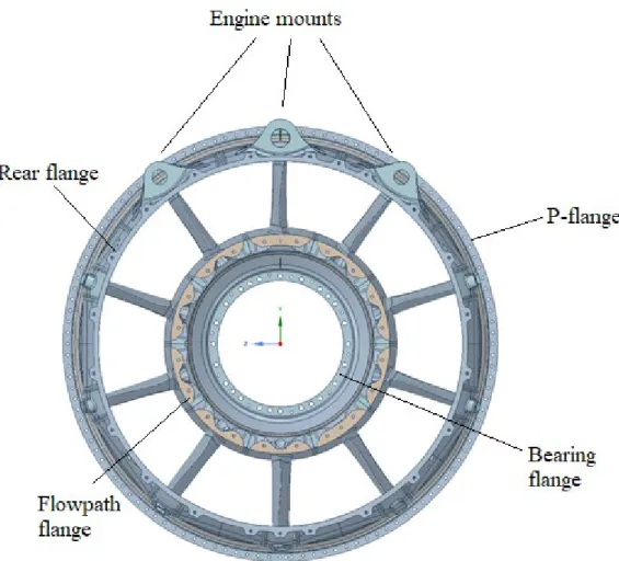
• Manufacturing cost drivers were identified for a specific TRS design, the geometry of this component is shown in Figure 1. The TRS in Figure 1 corresponds to a high bypass turbofan engine designed to generate about 133 kN of thrust.

• Manufacturing cost drivers for bolted flanges with standard geometries are investigated, which are relevant for aero engine applications.

• Manufacturing costs drivers for in-process inspection, heat treatments and cleaning are not considered in this project.

• Flanges made of Inconel 718, manufactured by forging and only material removal operations were the focus of this project.

• The cost modelling methodology incorporates lifecycle cost, and structural performance evaluations to better understand the tradeoff among them.

• The measure of flange structural performance was restricted to the amount of axial deformation it undergoes when loaded.

(15)

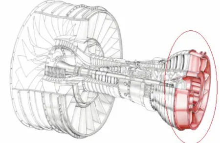
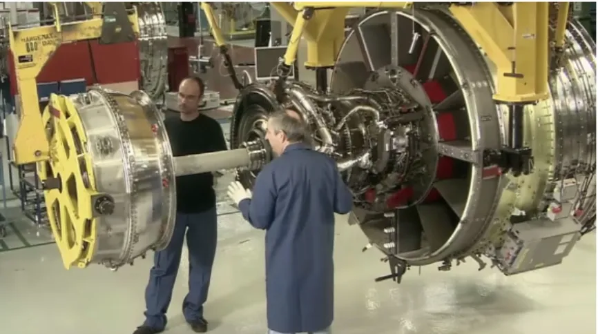
Illustrated in Figure 1 is a rear view of the TRS and in Figure 2, in red is the TRS represented in the context of a full jet engine assembly. Some important characteristics of the TRS are that it is a static structure, located at the engine exit, it guides the flow of combusted gases out of the turbine to the atmosphere and supports the jet engine at the rear by means of the three engine mounts, shown in Figure 1. The TRS, is assembled axially by means of four different types of flanges to the adjacent engine systems, these are shown also in Figure 1. The size of the TRS is driven by the size of the engine, as a result, the flanges in these structures will generally have variable dimensional requirements.

Figure 2: The TRS represented in red in the context of a typical high bypass turbofan engine assembly (Levandowski, 2014)

1.4 Methodology

In this project, due to confidentiality, computer simulated experiments were used to generate data as a series of CAD design cases of forged flanges. The generated design case studies were then analyzed with cost modelling techniques available in the literature (Hueber, 2016). The activities carried out in this thesis are here presented in order:

1. List the manufacturing sequence of forged flanges at GKN and define sub processes. 2. Identify cost drivers and parametrize flange geometry in CAD.

3. Define the responses of interest and models for analysis. 4. DOE set up with DesignXplorer.

1.4.1 List the manufacturing sequence of forged flanges at GKN and define sub processes

The manufacturing sequence of forged flanges for a TRS corresponding to an engine in the 133 kN thrust category was investigated at GKN in Trollhättan. This information was compiled with the help of Process Engineers, experts in the manufacturing of custom forged flanges. The manufacturing process was inspected, and two sub processes were extracted for further treatment. At this initial phase of the project, a bottom up cost modelling technique along with expert judgment (Hueber, 2016) was implemented to build up the manufacturing sequence.

1.4.2 Identify cost drivers and parametrize flange in CAD

The reason for defining sub processes in the manufacturing sequence, was that it simplified the identification of cost drivers and helped in the definition of two independent types of CAD

(16)

model parametrizations for DOE case studies. The first CAD model corresponds to a first group of cost drivers, turning operations performed on the forging envelop of flanges, and the second CAD model corresponds to the final set of material removal operations performed on forged flanges.

1.4.3 Define the responses of interest and models for analysis

The responses of interest are cost, structural performance, and weight. The three responses were evaluated as variations with respect to a nominal dummy flange design (baseline) to protect GKN’s technical data in this document. The cost was measured in terms of manufacturing complexity, lifecycle cost, forging cost and machining (turning) times. The performance was measured as the axial deformation of the flange. And the weight was directly obtained from all CAD model.

Due to the three different types of response, namely cost, performance and weight certain models for data evaluation were chosen. To evaluate the first DOE, parametric cost models featuring two Cost Estimating Relationships (CERs), property of GKN, were chosen. The second DOE was evaluated with the manufacturing complexity cost model introduced in section 2.4.5 and the lifecycle cost. As for the performance, the axial deformation was evaluated with the Finite Element Analysis (FEA) modules available in ANSYS Workbench.

1.4.4 DOE set up

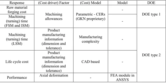
The parametrized flange geometry, in NX, was exported to the DesignXplorer toolbox in ANSYS Workbench, discussed in section 3.4, and a number of different design case studies (flanges) were generated in the form of DOEs. Two different DOE types were set up with DesignXplorer using the Latin Hypercube Design method. Table 1 shows a collection of factors, responses and models, this compiles the type of DOE studies that were carried out in the project.

Table 1: Collection of factors, responses and models for DOE case studies

Response (Cost driver) Factor (Cost) Model Model DOE Raw material

forging cost _Machining

allowances Parametric - CERs (GKN proprietary)

- DOE type 1 Machining (turning) time (FSM and ISM) - Machining (turning) time (LSM) Product manufacturing information (dimension and tolerance) Manufacturing complexity - DOE type 2 Life cycle cost

Product manufacturing information (dimension and tolerance) CAD based -

(17)

2 FRAME OF REFERENCE

This chapter presents a brief literature survey of the knowledge base used in this project with an emphasis on cost modelling methodologies.

2.1 Aircraft engines

Modern air travel would not be possible without the generation of thrust by jet engines in commercial and military aircrafts. Jet engines or gas turbines are propulsion systems that accelerate large amounts of fluid, typically air at atmospheric pressure, to produce an enormous reaction force back on the propulsion system to ultimately push the aircraft forward and make it fly (NASA 2014). The jet engine is essentially an application of Newton’s third law of motion, which states that “for every action there is an equal and opposite reaction”.

In a jet engine, the air travelling through the propulsion system will pass by different stages of turbomachinery (Torenbeek, Egbert 2013). At the air intake of the engine, a fan will suck fresh air from the atmosphere and guide it towards the compressor. The axial compressor, consisting of rotating and static blades assembled on to a shaft will raise the pressure of the air and decelerate it. The compressed air is then mixed with jet fuel and ignited with spark plugs to induce a combustion process. The chemical reaction takes place in a combustion chamber, which precedes another set of static and rotating blades assembled on to a shaft, called the turbine. The turbine blades are attached to the same shaft that drives the compressor. Finally, the exhaust gases after the combustion process will expand in the turbine and exit the engine through the nozzle.

As for the types of jet engines that have been developed over the years, these differ primarily in the way in which the energy conversion process takes place inside the engine to set the aircraft in motion (Rolls Royce 2005). Some relevant types of jet engines are presented in Figure 3 to Figure 6.

Figure 3: Double-entry single-single stage centrifugal turbo-jet (Royce, 2015)

(18)

Figure 5: Twin-spool turbo-shaft (with free-power turbine) (Royce, 2015)

Figure 6: Triple-spool front fan turbo-jet (high by-pass ratio) (Royce, 2015)

The triple spool front fan turbo-jet, as it was called by Rolls Royce, in Figure 6 is the jet engine of choice for modern commercial airliners. Nowadays, these engines are better known as “high bypass turbofan engines” because the “bypass” principle introduced in this solution, has increased vastly. The advantages of these engines is lower fuel consumption, decreased noise levels and high thrust (El-Sayed, 2008).

High bypass turbofan engines operate fundamentally like any other gas turbine, where air is compressed, burned with fuel and allowed to expand to generate thrust. The difference in the “high bypass” architecture is the large diameter of the fan in relation to the core of the engine that precedes the first compressor stage. These layout is better illustrated in Figure 2.

In the engine depicted in Figure 2, the fan pressurizes air, most of which bypasses the engine core to be accelerated and ultimately ejected through a nozzle at the rear of the engine. The secondary flow that goes into the engine core is compressed, burned with fuel and expands in the turbine to drive the fan to maintain a continuous engine cycle.

The dominating OEMs for jet engines have been working with “bypass” technology since the 1950s, when Rolls Royce introduced the first bypass turbofan engine, the Conway (El-Sayed, 2008). In recent times, OEMs have transitioned towards higher bypass ratios to produce efficient, cleaner and quieter engines. A collection of the most widely spread high bypass turbofan engines, their respective application and some technical specifications is reported in Table 2 for illustration.

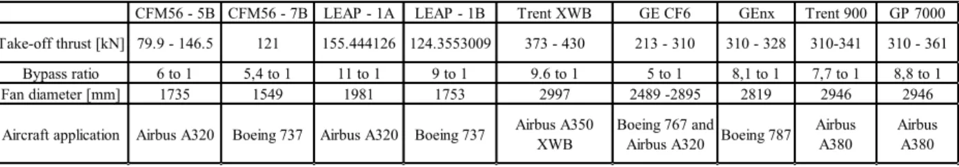
Table 2: Most popular high bypass turbofan engines and their application (Rolls, Trent 900, 2019) (CFM, 2019) (GE, 2019) (Safran A. , 2019) (Rolls, Trent XWB, 2019)

CFM56 - 5B CFM56 - 7B LEAP - 1A LEAP - 1B Trent XWB GE CF6 GEnx Trent 900 GP 7000 Take-off thrust [kN] 79.9 - 146.5 121 155.444126 124.3553009 373 - 430 213 - 310 310 - 328 310-341 310 - 361 Bypass ratio 6 to 1 5,4 to 1 11 to 1 9 to 1 9.6 to 1 5 to 1 8,1 to 1 7,7 to 1 8,8 to 1

Fan diameter [mm] 1735 1549 1981 1753 2997 2489 -2895 2819 2946 2946

(19)

2.1.1 Frames and cases for aircraft engines

All machine elements in a gas turbine engine are contained and surrounded by multiple casings, along the length of the engine. At the front of the engine, the fan and low-pressure compressor are contained by a fan case. In between the high- and low-pressure compressor, there is an intermediate case. A high-pressure compressor case for the last stage of air compression, a diffuser case and combustion case. At the rear of the engine, a high- and a low-pressure case for the high- and low-pressure stages of exhaust gas expansion in the turbine. Lastly, a Turbine Rear Structure (TRS) to support the engine at the back of the engine (Government of Canada 2018). The TRS as mentioned in the introduction of this document, is a product in the GKN Aerospace Engine Systems catalogue and in the context of a high bypass turbofan engine is located at the rear as a part of the low pressure turbine assembly, as it is illustrated in Figure 7. Figure 7 shows how the low pressure turbine assembly (left) is fastened to the fan and compressor modules (right).

Figure 7: Assembly operation of the low pressure turbine assembly module (left), fan and compressor modules (right) (Safran, 2019)

2.2 Bolted joints for aero engine frames and cases

The naming of bolted joints derives from the direction of the load they are subjected to (Bickford 1995). This means that when bolted joints are acted upon a load that is parallel to the bolt axis, they are called tension joints and bolted joints acted upon a load that is perpendicular to the bolt axis are called shear joints. Those joints loaded by a combination of tensile and shear loads will be named according to the load with the largest magnitude.

A designer relies on bolted joints to generate a clamping force between structures. For example, in view of this work, bolted joints generate clamp between airframe structures. The flanges in this type of applications must remain in contact to prevent undesirable leakages under normal engine operation and remain intact during ultimate operations (Czachor, 2005).

2.2.1 Tensile and shear joints

In general, it is desired for bolts in a tensile joint to clamp the joint members as much as possible to avoid any form of separation or slipping. Clamp loss is an undesirable phenomenon that can occur due to shock loads, thermal differentials and vibration in-service (Verein Deutscher Ingenieure 2015). In addition, bolts remain protected from fatigue failure if the tensile load is as

(20)

high as possible. Nevertheless, these could in some cases cause the bolted connection to fail due to stress.

There are two key aspects of a bolted joint when loaded primarily in tension. The clamping force in the joint members will affect the correct behavior of the joint and the tension in the bolt will affect the life of the bolt itself (Bickford 1995). Neither of the two characteristics of a bolted joint should be neglected for a successful application of the system. These two forces in the joint arise during assembly. The turning of a nut or bolt will exert tension in the bolt causing it to stretch and the joint elements to compress.

Bolt tension and clamping forces are not affected when shear loads are present, unless those loads are high enough to cause joint failure (Moss 2013). In other words, the unfavorable conditions in which a shear joint operates during service are typically less compared to those of a tensile joint.

2.2.2 Bolted joints for TRS

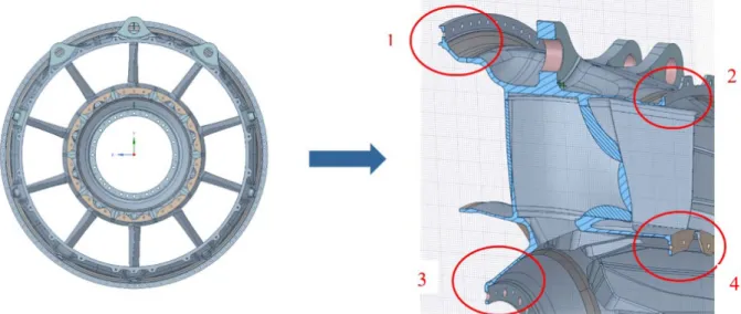
Jet engines in commercial aircrafts require a special type of bolted joint to safely connect components. When dealing with cylindrically shaped casings or rotors, the connection is carried out by a series of bolts and nuts placed in the circumference of the structure throughout the flange. In the case of a static structure as is the TRS, bolted flanges are located in places illustrated in Figure 8.

Figure 8: Two views of the TRS, the P-flange (1), rear flange (2), bearing flange (3) and flow path flange (4). The numbers in brackets refer to the number in the image.

Bolted joints in jet engine applications behave as they normally would in any other industry, if, they are subjected to normal operating conditions. However, with the introduction of high-bypass turbofan engines, more demanding constraints have also been introduced to the design of bolted joints (Czachor 2005). In addition, temperature variations, weight saving, and packaging have introduced tougher requirements to the dimensioning of bolted joints for high bypass turbofan engines.

Preload

(21)

improve the assembly clamp which include use of special tooling and synthetic lubricants (Czachor 2005).

There are three undesirable effects, which reduce clamp when the engine is operating. The first reason for clamp reduction is thermal dilation of the elements in the joint, that may not have the same material thermal properties, or because the operating temperature is varying. The second reason is due to flange contraction. The internal pressure of the fluid contained in the engine carcass introduces hoop stresses and stress in the radial direction due to temperature differences generates flange contraction (Verein Deutscher Ingenieure 2015). The third reason is due to the elastic modulus relation to temperature of the elements in the bolted joint.

Loading

The loading in bolted joints for turbofan engine applications is unique. The types of loads encountered during engine operation can be asymmetric, axisymmetric and in the worst-case impact loads. The asymmetric loading is a result of aircraft maneuvers, force imbalances due to parts in rotation, aerodynamics and thrust which causes bending because the engine mounts react to it at an offset from the engine centerline (Czachor 2005). The axisymmetric loading acts in the direction that is normal and transversal to the axis of the engine. These loads are a result of rotational speed, fluid pressure, torques and temperature differences. The third and worst type of loading for bolted joints is impact, which is due to unfortunate events where pieces of blade may break apart and hit the carcass near the flange.

Design for normal operating conditions

The design criteria for bolted joints in turbofan engines is a combination of loading conditions and the situation in which the engine is operating (normal or ultimate). Under normal operating conditions, typically the design of bolted joints must fulfill the following criteria:

• Adequate level of stiffness is to be maintained in the joints, so that the cyclic loading is reduced, and the life of the bolt improved for fatigue.

• Adequate length of the bolt shall be maintained to aid in joint stiffness, also because these allows for good properties under ultimate load operation.

• Adequate clamp levels for good Life Cycle Fatigue (LCF), joint stiffness, and sealing capacity.

• Adequate flange coefficient of friction at the interphase to prevent movement that can induce failure. Lastly any form of movement regardless of its amount is undesirable since it leads to wear and ultimately failure of the joint.

Design for ultimate operating conditions

Flange compliance with ultimate operating condition requirements can be verified using experimental tests. However, reproducing the conditions for this type of failure is hard and expensive. The alternative is to generate virtual models of flanges and bolted joints to perform Finite Element Analyses and predict ultimate failure (Czachor 2005). However, it is important to verify and validate the simulated results using component tests (experimental measurements).

(22)

2.3 Forged flanges for frames and cases

Typically flanges are manufactured from Inconel 718, a heat resistant nickel-based super alloy, with excellent mechanical properties, weldability, as well as, high temperature resistance (Mouritz 2012). This research has been restricted to forged Inconel 718 flanges, the raw material is generally received from the supplier in the shape of a ring and partially machined into a squared cross section. Subsequently, it goes through intermediate and final machining operations

2.3.1 Ring rolling

Ring rolling is the typical manufacturing process of choice for the production of flanges for aero engine frame and casing applications. The process consists on creating a hole in a bar of heated material to generate a ring-shaped piece for subsequent rolling (Bolin 2005). The ring at high temperature is rolled in a set up like the one in Figure 9. The piece is positioned in place with the mandrel fitted to the hole of the ring. The forming process starts when the main roll is made to rotate and is pushed against the work piece. Because of the friction between the main roll and the ring, the mandrel and the ring rotate as well. Progressively the ring will experience a reduction in radial thickness and the ring circumference in contrast will grow due to the change in cross section of the ring. The length along the axis of rotation of the ring can also be controlled by means of other type of tooling, shown in Figure 9. These are called axial rolls.

Figure 9: Illustration of a ring rolling process. (Bolin, 2015)

2.3.2 Machining Operations

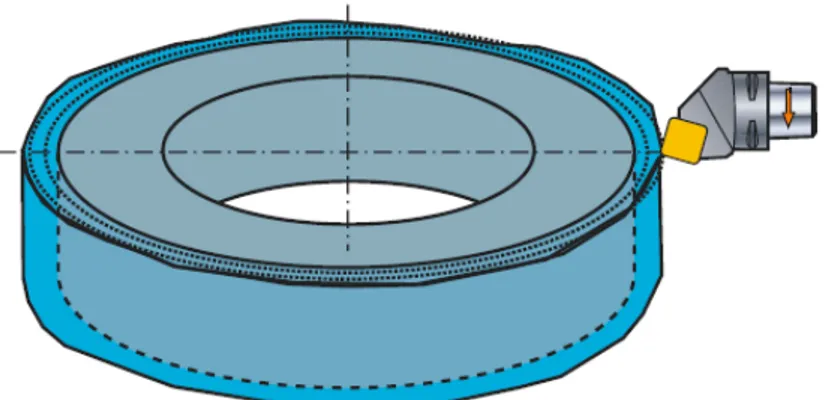
The machining operations, particularly turning, required to form squared cross-sectional rings into L-shaped profile flanges in aero engine structures, as illustrated in Figure 8, can be split into three distinct stages. These are characterized with respect to the type of tooling and surface requirements of the component. These three turning stages are referred to as first, intermediate and last machining stage, as illustrated in the Sandvik technical guide (Sandvik Coromant 2010). The first machining stage, illustrated in Figure 10, is an initial material removal process, where the skin and scale are removed from the surface of the forged ring of Inconel 718. This is essentially a cleaning process, that is carried out when the ring has been forged and it is in soft conditions. After a layer of material is removed, the flange will not have accquired its

(23)

Figure 10: Representation of the skin and scale material removal processes in forged rings, corresponding to the FSM (Coromant, 2010)

Figure 11: Representation of the ISM material removal process (Coromant, 2010)

The intermediate machining stage, illustrated in Figure 11, is the second material removal step in the manufacture of flanges. The first machining stage removes less material, than the intermediate machining, and it is carried out after the ring has undergone heat treatment right after being cleaned in first machining stage. At the end of this stage, the flange will have an L-shaped cross section ready for final machining.

The last machining stage is the step to shape the flange into its distinctive shape. This process removes the least amount of material from the flange because it is mostly concerned with obtaining a high-quality surface for the part (Kumar 2018).

2.4 Cost Modelling

In the literature (Hueber 2016), different classifications of cost modelling techniques are found. In this work the classification in three categories has been adopted, which consists of a parametric, analogous and bottom-up approach. These categorizations are the most popularly adopted in the literature (Hueber 2016). With this form of distinction, it is possible to trace back the existence of all other models to either one of the three mentioned models or a combination of them meaning that they may share some characteristics.

2.4.1 Parametric method

The idea behind parametric cost estimation methods are CERs. These are usually mathematical functions that allow the estimate of costs through dependent variables also referred to as parameters or cost drivers, which are essentially quantifiable characteristics of the product. For

(24)

instance, in this project flange geometrical features and manufacturing sequence operations are cost drivers.

The product cost will usually correlate to multiple product cost drivers. For instance, when a product is larger in size and volume the cost is also higher. Moreover, high correlating parameters are sought after to derive reliable CERs. Engineers will derive more than one CER for a complete cost estimate of the product.

The CERs of parametric cost estimations are typically implemented at initial design stages. It is advantageous to use this technique because the evaluation of costs is quick and straightforward when the analytical relationships are available (Duverlie 1999). However, this technique depends on a well-structured database of the history of the product for which an estimate is required. In other words, estimates are valid if they are made within the database’s range, beyond that range estimates might be highly inaccurate.

2.4.2 Bottom-up method

In this technique the steps of a manufacturing sequence, direct material, overhead, etc. are summed up to estimate the product cost. Cost estimates of this type are highly dependent on an in-depth knowledge of the product design, manufacturing sequence and the logic behind this production sequence. With this method it is possible to illustrate the product cost in detail since a very detailed input is fed into the model.

A bottom-up cost estimate can be carried out based on either the manufacturing sequence or design features of the product. Working with the (geometrical) design features of the product is particularly advantageous for product design because the implications of cost-sensitive decisions at early design stages are better understood (Hueber 2016). A good understanding of design choices is positive feedback to design engineers with the aim to improve the development and design process of the product.

Unfortunately, bottom-up estimates depend on very detailed documentation of the product. Similarly, this technique requires a lot of effort to output an estimate due to the large amount of data that needs to be handled. In contrast, this method is straightforward and applicable to old and new products and technologies. In fact, it is the only cost estimating method that can be used on new products and manufacturing technologies.

2.4.3 Analogous method

The principle behind analogous cost estimation is to use similarities among existing products to adjust to the unknown product cost. Product cost estimates are carried out assuming products with similar features in their design result in similar costs. Once again, this technique requires structured databases of more than one product since the unknown product cost is estimated by looking into the similarities and differences of at least two cases. The outcome of this method is a good cost estimate for less effort when compared to the previously presented methods. Typically used in initial stages of the design process.

Expert judgement is necessary in this technique to identify similarities and differences among previous project cases and new projects. With an extensive database a reference cost model can be built so that the new product is fitted in the reference as a mathematical model. With the reference the manufacturing costs can be estimated according to the main attributes that are

(25)

2.4.4 Expert judgement

An additional type of cost estimation approach that does not belong to either of the three previously mentioned categories is a cost engineer’s experience. Experienced engineers can provide rules of thumb for estimation. This knowledge is unique because the origin and justification for the information is not always clear or reproducible by anyone else. This method comes in handy, when there is a lack of information and structured databases. In fact, if no costing structured database exists, the only option is to rely on expert judgement (Rush 2001).

2.4.5 Complexity theory method

In 1948, Claude Shannon introduced information theory in his paper “A mathematical theory of communication”. The theory was not intended to handle cost estimation tasks, but researchers concerned with manufacturing costing methods claim that product definition (information) provides better cost estimates than the previously introduced techniques in this chapter.

Another group of researchers claim that product information is a direct cost driver to manufacturing cost and works better than cost models based on weight or material parameters. In addition, a cost estimating approach based on information theory is particularly interesting to designers because it allows them to use the technique as a communication channel between design and manufacturing.

The work carried out by (Collopy 2001) at Rolls-Royce showed that manufacturing costs can be estimated from dimensions in technical drawings. Collopy and Eames base their work on what (Hoult 1996) demonstrated. Hoult and Muter discover interesting correlations between machining times for certain processes, and product information. It turns out that the quantity of information reported in a technical drawing is proportional to the machine processing time. Furthermore, in Volume 20: Materials Selection and Design of the ASM Handbook (Hoult & Meador, 1997), the authors discuss some of the aspects of their research carried out to correlate machining times and the complexity of parts.

The previously mentioned references also discuss the method to measure information. Deriving from Shannon’s information theory, the proposed algorithm to measure information is the following: Equation 1: 𝑀𝑀𝑀𝑀𝑀𝑀𝑀𝑀𝑀𝑀𝑀𝑀𝑀𝑀𝑀𝑀𝑀𝑀𝑀𝑀𝑀𝑀𝑀𝑀𝑀𝑀 𝐶𝐶𝐶𝐶𝐶𝐶𝐶𝐶𝐶𝐶𝐶𝐶𝐶𝐶𝑀𝑀𝑀𝑀𝐶𝐶 = ∑ 𝐶𝐶𝐶𝐶𝑀𝑀2𝑑𝑑𝑑𝑑𝑑𝑑𝑑𝑑𝑑𝑑𝑑𝑑𝑑𝑑𝑑𝑑𝑑𝑑_{𝑡𝑡𝑑𝑑𝑡𝑡𝑑𝑑𝑡𝑡𝑡𝑡𝑑𝑑𝑡𝑡𝑑𝑑}𝑘𝑘 𝑘𝑘 𝑁𝑁 𝑘𝑘=1

Where N stands for the total number of specified dimensions in a technical drawing, and k stands for the kth_{dimension or tolerance out of the total. The formulation, dating back to (Shannon}

1948), has not been further investigated in the context of manufacturing cost estimation. However, Collopy and Eames’ research showed that the cost modelling predictive potential with this formulation is comparable to the accuracy of previously mentioned cost estimation techniques.

The formulation states that all dimensions that define the product’s manufacturing process are normalized with respect to its tolerance. The practice of using the logarithm base two dates to Shannon’s work, and it is a way to numerically represent the number of bits necessary to define the product’s manufacturing process.

(26)

2.5 Design for manufacturing and assembly

Because design for manufacturing (DFM) and design for assembly (DFA) practices are aimed at cost reduction, these principles were outside the scope of the project and a detailed discussion of these is omitted. However, the fundamental engineering practices of DFM and DFA were a starting point to identify cost drivers in the manufacture of bolted flanges for the TRS in 133 kN thrust category. Reviews on DFM and assembly, as well as, design best practices have been cited in the literature, such as (Andreasen, Kähler, & Lund, 1982) and (Kobe, 1990).

The pioneers and developers of the DFA methodology, (Boothroyd & Dewhurst, Product design for assembly, 1986) discussed how proper assembly systems enable the most economical product designs from an assembly perspective. In (Boothroyd & Dewhurst, Design for assembly - a designers handbook, 1983) they critique parts according to their ease of insertion and handling. Different DFA approaches have been proposed since its introduction at the end of the 1970s, but the principles of DFA have remained same.

In (Corbett, 1987) a list of principles to implement DFA in product design is illustrated. The principles are listed in two categories: (1) Number of parts, fixtures, design variations, assembly directions and movements should be minimized. (2) Adequate access for locating operations, symmetry of parts, simplified manipulation and visibility should be possible.

Following the development of DFA, (Stoll, 1986) explored the DFM concept in an attempt to concurrently consider the function of a product design and the processes required to manufacture it. Just like (Corbett, 1987), Stoll wrote guidelines intended to provide systematic best design practices for DFM. Stoll 1988 claims that the “use of this (DFM) human-oriented knowledge, helps narrow the range of possibilities so that the mass of detail which must be considered is within the capacity of the designer and planner”.

The list of guidelines for DFM in Stoll’s work are to: (1) minimize number of parts, (2) aim for modular designs, (3) use standard components, (4) design parts to serve multiple functions, (5) design parts for multiple use, (6) design parts for simple fabrication, (7) avoid separate fasteners, (8) minimize assembly directions, (9) maximize design compliance to address imperfections, and (10) minimize part handling

When a nominal flange design for a TRS is examined under the DFM and DFA scope formulated by (Corbett, 1987) and (Stoll, 1986), a few things can be stated. Flange design clearly involves multiple standard parts, the use of separate fasteners is inevitable due to large flange diameters, flanges and the TRS are assembled uniaxial, assembly movements are minimal, there is good accessibility for bolt and nut fastening, flanges and the TRS tend to be symmetric components, flanges serve multiple functions, for example axially locating the TRS and sealing the inner flow path.

2.6 Experimental design - DOE

With limited time and resources, it can become challenging to learn about a product or a process without setting up the right experiment. An adequately designed experiment or DOE is useful to strategically plan an experiment to effectively and efficiently obtain a better understanding of the process in question. In engineering, DOEs have become common practice to speed up the

(27)

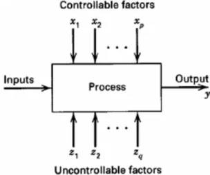
Designed experiments are used to investigate a system, which receives input variables, and delivers an output. Inputs are also referred to as factors and outputs are also referred to as responses of the system. Not all the inputs to the system are the same, there will always be factors that the experimenter is able to control and factors that the experimenter cannot control. An adequately designed experiment will take into account all the factors and how these affect the system’s response (Jiju 2003).

To design an experiment (Montgomery 2013), proposes a series of steps to follow. These steps are presented below:

• Problem statement (Research question) • Define factors, levels and ranges • Define responses

• Conduct the experiment • Analyse response

• Conclusions and reflections

Figure 12: Graphical representation of the process in a DOE (Montgomery, 2013)

2.6.1 Classic and modern

Various types of designs within the DOE domain were developed as a result of a need for continuous improvement in effectivity and efficiency of physical experimentation (Kleijnen 2015). Over the years, designs like full, half factorial, central composite, Box and Bhenken took shape and were aimed at physical experimentation only; these type of designs are denoted in the literature as classical DOEs (Sushant 2017).

Nowadays, due to the rapid development of computational power and speed, researchers and engineers from various disciplines can opt for alternatives to traditional physical experimentation. The alternative is to use economic and reliable computer simulations that generate data sets at the expense of a real system experimentation. Unfortunately, because physical and computer experiments are fundamentally different, a direct application of classical DOEs to computer experiments is not immediate.

The need to handle computer simulated experiments adequately, inspired another wave of development, which focused on new designs, in the literature these are called modern DOEs

(28)

(Sushant 2017). This family of DOEs, does not deal with the random nature of physical experiments, but with the deterministic nature of computer simulations. The main difference between classical and modern DOEs is that, modern DOEs do not assume first and second order system responses like most classical DOEs. Instead modern DOEs focus on defining the best sample points within a given domain to simulate the process response.

2.6.2 Latin Hypercube Design

One of the modern DOE techniques to handle computer simulated experiments is the Latin Hypercube Design (LHD) or Latin Hypercube Sampling (LHS). Latin hypercube design is a method to generate a random sample of points from a set of parameters resulting from a multidimensional distribution. This technique was introduced by (Olsson 2003) and became popular because it enables a reduction in computer processing time without compromising accuracy in the results compared to one of the first modern sampling techniques, Monte Carlo. A second advantage of LHS is that it introduces a level of variability that resembles a more traditional physical experiment.

(29)

3 METHOD

The method proposed in this project for cost modelling and tradeoff studies is developed in this chapter

3.1 List manufacturing sequence and define sub processes

The manufacturing sequence for forged flanges was compiled by receiving input from Process and Design Engineers at GKN. A meeting was arranged and a survey was carried out to gather information regarding the processes (Aronsson & Widström, 2018). A list of questions that were discussed at this meeting is found in appendix A. With these input and a bottom up cost modelling technique (Huebel 2016) the manufacturing sequence was put together. In other words, expert judgement and a bottom up cost estimating approach were combined and implemented at the initial stage of this project.

The bottom up cost modelling technique helped breakdown the input received from the Engineers into well-defined manufacturing steps. The resulting manufacturing sequence was then used as raw input for further use in the project. The manufacturing sequence was examined and operations were allocated into groups that are called sub processes in this document. The allocation task was based on the criteria that manufacturing steps of similar manufacturing technology characteristics belong to the same sub process.

The method of defining sub processes within a manufacturing sequence is illustrated in Table 3 and Table 4. A sample manufacturing sequence in Table 3 is divided into a number of sample sub processes numbered 1 through 4 in Table 4. Notice that the operations in Table 4 for sub process 1 through 4 were grouped according to the criteria mentioned above, similar manufacturing technology characteristics.

Table 3: Sample manufacturing sequence

Manufacturing sequence Marking 1 Turning 1 Turning 2 Turning 3 Inspection 1 Inspection 2 Cleaning 1 Welding 1 Heat treatment 1 Turning 4 Turning 5 Turning 6

Table 4: Sample sub processes

Sub process 1 Sub process 2 Sub process 3 Sub process 4 Turning 1 Inspection 1 Cleaning 1 Weld 1 Turning 2 Inspection 2 - Weld 2 Turning 3 - - -

(30)

In the same way, the tables in Appendix B show the actual manufacturing sequence constructed for forged flanges at GKN and the definition of sub processes.

3.2 Identifying cost drivers and parametrization of flange

geometry

The second task of this project consisted on identifying cost drivers for sub process 2 and 4 in Appendix B and turn these into parametrized CAD models for flanges. The other sub processes in Appendix B were not investigated further because the operations allocated in them were outside the scope of the project. The identified cost drivers for sub process 2 and 4 are shown in the third columns of Table 5 and Table 6. These sub processes were formed based on the type of tooling and surface finishing requirements of the flange at specific stages of the manufacturing process, as proposed by Sandvik’s technical guide.

Table 5: Collection of operations allocated in sub process 2

Operation

number Sub process 2 Cost drivers

2 Cleaning -Flange outer and inner

diameter

-Thickness of flange -Double blend of flange -Snap fit

-Size of forging envelop -Machining allowances 3 Rough turning

4 Turning outer diameter (fine)

5 Turning inner diameter 6 Turning axial length

7 Deburring

29 Deburring

Table 6: Collection of operations allocated in sub process 4

Operation

number Sub process 4 Cost drivers

22 Turning outer diameter -Flange outer and inner diameter

-Thickness of flange -Double blend of flange -Snap fit

-Machining allowances 23 Turning front face &

press fit

24 Turning aft face

25 Milling

26 Drilling

27 Chamfer

The cost drivers reported in Table 5 and Table 6 were then associated to two representative CAD models, one for each sub process. The results of the parametrization are illustrated in Figure 13 through Figure 16. The aim of the parametrization task was to collect information from the cost drivers into a representative CAD model to be analyzed with a DOE platform at a later stage in the project, this is discussed in the next section of this chapter.

Figure 13 illustrates the parametrization of a forging envelop, for a nominal flange, this corresponds to sub process 2. For this case study, six parameters were defined to investigate the

(31)

weld deformation, heat treatments, etc. Due to confidentiality, a detailed discussion of these machining allowances is omitted.

Figure 13: Forging envelope parametrization and parameters

Figure 14 and Figure 15 illustrate the parametrization of a flange with final product definition in the form of sketches, this corresponds to sub process 4. For this case study, fourteen parameters were defined to investigate the cost drivers from Table 6. The parameters in this case represent the geometrical design features of a typical flange for a TRS. For clarity, Figure 16 illustrates the end result of the parametrized sketches in Figure 14 and Figure 15.

(32)

Figure 15: Final machined flange parametrization (front)

Figure 16: End result of final machined flange parametrization

3.3 Define responses and models for analysis

The responses of interest in this project were the cost, structural performance and weight. Because the manufacturing sequence was divided into sub processes, the evaluation of these responses was independent for each one of them. The responses were evaluated with respect to a nominal flange design, this nominal design corresponds to the flange geometry of a TRS in the 133 kN thrust engine category. The reason for this approach was to understand the positive and negative effects of a cost driver on to the three responses and to protect the technical data made available by GKN.

3.3.1 Cost

The cost response for sub process 2 is the forging cost (raw material), first and intermediate turning operation times. As for sub process 4 the cost responses are the final machining turning operation time and the lifecycle cost. Table 7 collects the responses for the sub processes investigated, for clarity.

(33)

Table 7: Collection of responses for cost and models used for evaluation

Sub process Cost response Model Unit 2

Forging cost

Parametric-CER USD First and intermediate turning operation times

Parametric-CER Minutes 4

Final turning operation time Manufacturing

complexity - Life cycle cost Weight

tradeoff USD

The proposed model to evaluate the response of the forging cost was a parametric cost model because of the availability of CERs of the process at GKN due to data acquisition over time at the purchasing department. In the same way, the cost of the first and intermediate turning operations was evaluated with a parametric cost model (CER) of the process.

The final turning operation time was evaluated based on complexity theory. As mentioned in the second chapter, the complexity theory (Shannon 1948) supports that the manufacturing cost of a product can be estimated through the complexity of the final product definition. Typically, the product definition of a part is connected to the technical drawings that define it. A technical drawing is made up of multiple views, dimensions tolerances, annotations and symbols.

The model proposed by the complexity theory has been used to estimate the final turning operation time of flanges. To measure complexity, the only algorithm available in the literature and proposed by Shannon was adopted. Product complexity or final turning operation time was evaluated following these steps:

1. Collect technical drawings (product manufacturing information) which define the TRS assembly for the 133 kN thrust category.

2. Record all dimensions and tolerances in the drawing assembly of the TRS. 3. Evaluate the manufacturing complexity with Equation 1:

The complexity of the TRS assembly was evaluated with the aim to quantify a relative percentage of flange complexity with respect to the entire TRS, in other words, the amount of final turning operation time for flanges with respect to final turning operation time for the entire TRS. The result of this calculation is presented in the fourth chapter of this document.

For illustration, an example of how manufacturing complexity was calculated is here presented. The typical L-profiled flange drawing section view in Figure 17 will be used for illustration. The first step was to collect all dimensions and tolerances from all drawings that define the product, in this case the flange cross section in Figure 17. Then the proposed algorithm from Equation 1 is used to evaluate manufacturing complexity in the following way.

𝑀𝑀𝑀𝑀𝑀𝑀𝑀𝑀𝑀𝑀𝑀𝑀𝑀𝑀𝑀𝑀𝑀𝑀𝑀𝑀𝑀𝑀𝑀𝑀𝑀𝑀 𝑀𝑀𝐶𝐶𝐶𝐶𝐶𝐶𝐶𝐶𝐶𝐶𝐶𝐶𝑀𝑀𝑀𝑀𝐶𝐶 = � 𝐶𝐶𝐶𝐶𝑀𝑀2( 𝑁𝑁𝑁𝑁𝑑𝑑𝑁𝑁𝑑𝑑𝑡𝑡 𝑑𝑑𝑜𝑜 𝑑𝑑𝑑𝑑𝑑𝑑𝑑𝑑𝑑𝑑𝑑𝑑𝑑𝑑𝑑𝑑𝑑𝑑𝑑𝑑 𝑡𝑡𝑑𝑑𝑑𝑑 𝑡𝑡𝑑𝑑𝑡𝑡𝑑𝑑𝑡𝑡𝑡𝑡𝑑𝑑𝑡𝑡𝑑𝑑𝑑𝑑 𝑘𝑘=1 𝑑𝑑1 𝑀𝑀1) + 𝐶𝐶𝐶𝐶𝑀𝑀2� 𝑑𝑑2 𝑀𝑀2� + ⋯ + 𝐶𝐶𝐶𝐶𝑀𝑀2� 𝑑𝑑7 𝑀𝑀7� Where k stands for the kth _{dimension in the product manufacturing information of the drawing in}

(34)

Figure 17: Typical L-profile flange drawing (cross section view)

3.3.2 Structural performance

The structural performance was evaluated in terms of the axial deformation of a flange. In a flange for the TRS, the superposition of an axial, a shear, a moment and a torque on to the flange is typical. This type of nominal load case was replicated by setting up a “Static Structural” analysis in ANSYS Workbench. The parametrized flange from the previous section, for sub process 4 was assembled along with a “dummy flange” and a “bolt and nut dummy” to set up an FEA study. The assembly of these three solid bodies is shown in Figure 18.

The load case was set up in the following way: A simply supported constraint was defined on the labelled face of Figure 19 of the parametrized flange for sub process 4. On to the dummy flange, axial, shear, moment and torque loads were defined on its respective labelled face in Figure 19. Lastly a pretension was defined onto the labelled dummy fastener in Figure 19.

(35)

3.3.3 Weight

The evaluation of the weight was simply carried out in the CAD and FEA software tools. The density of Inconel 718, the assumed material for the nominal flange, was an input to the digital files and the estimated value from the software was output. Moreover, the weight was also considered a cost response. In sub process 4, the tradeoff in aircraft economy, 1 kg of finished product is equivalent to roughly $1000 of life cycle cost (LCC) was evaluated.

3.4 DOE set up – LHS

Two independent DOEs were set up for sub process 2 and 4 at this stage of the project. The parametrized CAD models for flanges were exported from the CAD software NX into the DesignXplorer platform. DesignXplorer is a tool within the ANSYS Workbench software package, which assists the user in design exploration studies. This tool works on the basis of design of computer experiments with system parameters as an essential part of it (ANSYS, 2018). Parameters can be typically generated in compatible CAD environments, system responses can be analyzed with the models available in the toolbox, and models that are input by the user.

Design points were generated for two DOEs using the LHS method introduced in section 2.6.2 within DesignXplorer. The design space generated for sub process 2 is illustrated in Table 8. As for sub process 4, unfortunately, due to an inadequate update of parameters in the CAD environment because of poor model robustness, responses for the fourteen parameters in Figure 14 and Figure 15 were not obtained.

A new design space was generated for the DOE corresponding to sub process 4 with a reduced number of parameters. The re designed DOE for sub process 4 is illustrated in Table 9. Unfortunately, a much reduced number of parameters had to be used. The issue was that the fourteen parameters in the CAD model conflicted with each other after every iteration of the simulation. When the number of parameters was excessive, the variables would interfere with each other and the CAD model generation would fail.

The parametric models (CERs) for cost and manufacturing complexity discussed in Table 7 were manually input to the solver in DesignXplorer, since these are not part of the ANSYS package. These expressions are specifically derived for the particular forging and machining processes at GKN.

For illustration, the solution workflow that was set up in ANSYS Workbench for the DOEs corresponding to sub process 4 is presented in Figure 20. As shown in Figure 20, the flange geometry in block A is sent to block B to set the thermal boundary conditions on the flange. In block C, the boundary conditions for the structural performance analysis are set. Lastly, in block D, the various design points from the DOE are iterated and solved for. A similar workflow is carried out for sub process 2, but for that case block B and C are omitted since no structural performance evaluation were carried out.

(36)

Figure 20: ANSYS Workbench workflow for evaluating DOE for sub process 4 Table 8: Design space and responses generated for sub process 2

(37)

(38)

(39)

4 RESULTS AND DISCUSSION

The results obtained for the case studies defined in chapter 3 are discussed in this chapter

4.1 Manufacturing complexity a measure of final machining

cost

To support the claims of the literature (Hoult & Meador, 1997) and extend the use of complexity theory to cost modelling of flanges, for a 133 kN thrust TRS, these first set of results is presented. The algorithm to estimate manufacturing complexity, proposed in the literature, was selected to calculate the TRS assembly complexity. The structure, which is part of this study, is currently in production at GKN, and it is fully defined, meaning that the assembly structure has fully defined technical specifications.

The product specification of the TRS consists of 24 drawing sheets, which make up the assembly drawing. The 24 pages were inspected individually, and all the dimensions and tolerances were recorded. The manufacturing complexity from each page was calculated based on the algorithm presented in chapter 2 according to Shannon’s work. The manufacturing complexity for the flanges was also estimated separately, with the aim to estimate the relative complexity with respect to the entire TRS.

Table 10 reports the relative flange complexity with respect to the total manufacturing complexity of the assembly. These results were verified with experienced engineers working with the TRS for many years (Aronsson & Widström, 2018). The input received from them suggests that the total relative flange complexity roughly corresponds to the cost incurred in the last stage of machining operations. This validation allowed the continuation of the work to estimate costs with the manufacturing complexity model.

Table 10: Manufacturing complexity measure for entire TRS final product definition

LPT

flange flangeRear Bearing flange ID flow path flange Total

Flange complexity 187 135 197 112 631

TRS complexity 2343

Relative flange complexity 8% 6% 8% 5% 27%

A last remark about this results, is that for the total relative flange complexity to experience a percentage change, either positive (increment in cost) or negative (reduction in cost), 11 units of flange or TRS complexity are required. In other words, if the assembly drawing technical specifications become either more or less complex due to design features and consequently dimensions and tolerances are changed, the measure of cost will be affected as well.

4.2 Final product definition flange geometry

– sub process 4

The cost response for the final product definition flange case study consists of two components, the manufacturing complexity and the aircraft LCC, both discussed in previous sections. The results for the cost are presented in Figure 21 and Figure 22, with respect to the parameters f1 and

(40)

f2. The response surface with respect to the parameters f1 and f2 is discussed because they have

shown the strongest correlation out of the four input variables to the DOE corresponding to sub process 4.

4.2.1 Manufacturing complexity and aircraft lifecycle cost

The manufacturing complexity response surface is shown in Figure 21. This surface is plotted for the design space generated by f1 and f2. It is expected for this response surface to have a

logarithmic nature, since the manufacturing complexity algorithm is implemented based on a logarithm of base two, as suggested in the literature (Shannon, 2001). The range of values for the change in manufacturing complexity is somewhat limited as seen in Figure 21. We say it is limited because it ranges between -1 and -3.5 units of complexity. Recalling the final remarks of the first section in this chapter, it is required to have at least a change of 11 units of complexity to perceive a significant change in the cost for the final machining operation of flanges.

The design space illustrated in Figure 21, suggests very little room for cost reduction opportunities if that is the aim. However, the results could also be interpreted by saying that the double radii (f1 and f2) of the standard flange design have a small impact on the cost of final

machining operations of flanges. With this information, efforts could be taken to focus the attention on other design attributes of the flange geometry.

Figure 21: Manufacturing complexity for radii 1 and 2

4.2.2 Aircraft lifecycle cost (LCC)

The second contribution to the cost response is the weight of the standard flange design. This response is the aircraft lifecycle cost and it derives from the tradeoff mentioned in previous sections from the aerospace industry, which states that 1 kg of finished product is worth $ 1000 of LCC.

The aircraft lifecycle cost response is illustrated in Figure 22, this response is scalable to the weight, so a separate plot for the weight, is not presented. Figure 22, suggests that within the range of values for the radii f1 and f2 there is a large margin to save in aircraft lifecycle cost.

These results are expected because lower settings of the input variables f1 and f2 to the DOE

(41)

Figure 22: Aircraft lifecycle cost for radii 1 and 2

4.2.3 Performance – Directional deformation

The performance response surface is illustrated in Figure 23, this response is the change in directional deformation along the axis of rotation of the aircraft engine. As it is the case in the previous surface plots, the input variables f1 and f2 of the DOE are discussed. It is suggested in

the surface plot for the directional deformation that the factors in the DOE have a very small impact to the performance.

The input variables to the DOE, have a somewhat small influence to change the directional deformation of the flange. This suggests that a different setting of the dimensions of the rounds in the parametrized standard flange have the potential to reduce costs without a significant sacrifice in performance. This opens up the possibility to revisit existing flange designs that customers might find economically competitive.

(42)

4.3 Forging envelop, first and intermediate machining case

study – sub process 2

The results presented in this section refer to the comparative study carried out on a forging envelop design case, sub process 2.

4.3.1 Forging envelop cost

The two response surfaces in Figure 24 and Figure 25, correspond to the change in the cost of the forging envelop material (raw material) and the change in the rough machining cost i.e. the first and intermediate machining stage operations. The cost of the forging envelop was evaluated with CERs and the machining cost was measured in number of seconds required to turn the envelop volume during the first and intermediate machining stages, collectively. The parameters which feature the strongest correlation for the two response surface are p2 and p4.

Figure 24, suggests forging envelop volumes have the potential to be less cost intensive, if the machining allowances are revisited. It appears that the raw material cost of the forging envelop design has the potential to reduce the cost up to $150 if the machining allowances for the faces corresponding to p2 and p4, are controlled with tighter requirements.

This is an expected result, tighter machining allowances correspond to less material required in the forging envelop volume. This also means that smaller forging envelops have a smaller volume when the machining allowances are tight. As a result, less time is required in the first and intermediate machining stages of material removal.

(43)

Figure 25: Machining time for parameter 2 and 4

4.4 Answers to research questions

Up next an attempt to answer the research questions stated at the beginning of this document is presented:

What cost estimation models are available to map the manufacturing cost of forged flanges?

The cost estimation models available to map the manufacturing cost of forged flanges are parametric, analogous and bottom-up. These models propose classical cost estimation techniques for manufacturing operations, which have been used extensively in other industrial applications (Jung, 2002). It is important to note that the classification of cost models presented above is based on (Hueber, 2016). Other sources treating cost modelling might provide different classification strategies.

Can these models be implemented to map the manufacturing cost of forged flanges for a TRS?

The parametric, analogous and bottom up cost models can be implemented to estimate the cost of manufacturing processes given the correct requirements are present. Any of these three classic cost models are apt to be applied to forged flanges for the TRS. However, the requirements needed to apply any of these models are not completely satisfied yet.

The parametric model can be used, if CERs are identified for the processes involved in the manufacture of forged flanges. For instance, the scope of parametric modelling could be stretched, if CERs for ring rolling, rough machining, intermediate, final machining and welding are developed. As mentioned in section 2.4.1, CERs must be derived from historical data sets. It is beneficial to investigate past trends for similar flange designs in order to derive more CERs. The analogous model is suitable for the applications in this project. The design of forged flanges has been consistent through the years, few geometric features have changed. There is a wide range of past flange designs, with similar characteristics to new ones, that can be investigated

(44)

further. Creating a structured data set of legacy flanges could be beneficial for analogous cost estimation.

The bottom up cost estimation model is applicable to forged flanges that have a well-defined process manufacturing sequences. The manufacturing sequence that was put together in this project, and is presented in Table 11 can be used to implement the bottom up cost estimation model fully. The information that is missing is the cost that corresponds to each one of the manufacturing steps.

Is it possible to suggest a cost estimation model for flanges, to estimate the cost of design features?

The analogous model seems to offer the most attractive approach for cost modelling in the case of forged flanges. Since flanges have kept their geometric features essentially unchanged throughout the years, this modelling technique appears to be the most appropriate of the three. Alternatively, the manufacturing complexity method offers an extraordinary cost modelling approach with a lot of potential. The manufacturing complexity theory introduced in section 4.1, partially verified by Process engineers suggests that geometric complexity, design feature cost and final machining costs are connected through the complexity index.

Is the cost modelling approach suitable to carry out a comparative analysis among the performance, cost and weight?

The approach to cost modelling in this project attempted to merge different traditional cost estimating methods. The parametric, bottom up and manufacturing complexity index were used in parallel to handle the manufacturing cost from different standpoints. These three methods allowed the quantification of costs in a straightforward fashion.

The cost models were implemented to carry out comparative studies with the structural performance, and the weight. One of the shortcomings of this approach was the sacrifice in quality of the manufacturing cost estimation due to the simplifications for estimating the cost. Nevertheless, the method shows promising results to carry out further tradeoff studies when more mature cost estimation models are introduced.