Investigating different road safety implications of two TDM policy measures : Fuel-cost increase and teleworking

(1)

16th Road Safety on Four Continents Conference

Beijing, China 15-17 May 2013

0

INVESTIGATING DIFFERENT ROAD SAFETY IMPLICATIONS OF TWO

TDM POLICY MEASURES:

FUEL-COST INCREASE AND TELEWORKING

Ali Pirdavani

1

, Tom Brijs,

Tom Bellemans and Geert Wets

Transportation Research Institute (IMOB)

Hasselt University

Wetenschapspark – Building 5

B-3590 Diepenbeek, Belgium

Tel: +32(0)11 26 91 39

Fax: +32(0)11 26 91 99

E-mail:

ali.pirdavani@uhasselt.be

ABSTRACT

Travel demand management (TDM) consists of a variety of policy measures that affect the transportation system’s effectiveness by changing travel behavior. Although the primary objective to implement such TDM strategies is not to improve traffic safety, their impact on traffic safety should not be neglected. The main purpose of this study is to investigate differences in the traffic safety consequences of two TDM scenarios; a fuel-cost increase scenario (i.e. increasing the fuel price by 20%) and a teleworking scenario (i.e. 5% of the working population engages in teleworking). Since TDM strategies are usually conducted at a geographically aggregated level, crash prediction models (CPMs) that are used to evaluate such strategies should also be developed at an aggregate level. Moreover, given that crash occurrences are often spatially heterogeneous and are affected by many spatial variables, the existence of spatial correlation in the data is also examined. The results indicate the necessity of accounting for the spatial correlation when developing crash prediction models. Therefore, zonal crash prediction models (ZCPMs) within the geographically weighted generalized linear modeling (GWGLM) framework are developed to incorporate the spatial variations in association between the number of crashes (NOCs) (including fatal, severe and slight injury crashes recorded between 2004 and 2007) and a set of explanatory

1

(2)

1

variables. Different exposure, network and socio-demographic variables of 2200 traffic analysis zones (TAZs) in Flanders, Belgium, are considered as predictors of crashes. An activity-based transportation model is adopted to produce exposure metrics. This enables to conduct a more detailed and reliable assessment while TDM strategies are inherently modeled in the activity-based models. In this study, several ZCPMs with different severity levels and crash types are developed to predict the NOCs. The results show considerable traffic safety benefits of conducting both TDM scenarios at an average level. However, there are certain differences when considering changes in NOCs by different crash types.

1 INTRODUCTION

Urbanization and population growth together with employment and motor vehicle growth largely affect road transportation systems’ performance. To diminish the negative impacts, different policy measures and strategies have been applied by authorities. These programs and strategies that promote more efficient use of transportation systems are generally called TDM strategies (Litman, 2003). TDM strategies consist of several policies and strategies which aim to overcome transportation problems by means of mode shift (e.g. using public transportation instead of cars, biking for short distance trips or carpooling), travel time shift (e.g. avoiding traffic peak-hours by leaving home/the work place earlier or later) or travel demand reduction (e.g. teleworking) (VTPI, 2012). In general, TDM strategies are implemented to improve transportation systems’ efficiency. However, their potential secondary impacts such as traffic safety or environmental effects should not be overlooked.

The main contribution of this study is, therefore, to couple ZCPMs with two TDM scenarios; namely the fuel-cost increase and the teleworking scenario that are simulated in an activity-based transportation model called FEATHERS (Forecasting Evolutionary Activity-Travel of Households and their Environmental RepercussionS) (Janssens et al., 2007). This is carried out to evaluate the traffic safety effects of conducting such TDM strategies by means of a simulation-based analysis of the impact on the travel demand in Flanders, Belgium. This way, the behavioral impact of TDM scenarios in terms of traffic demand is incorporated in the analysis. By assigning traffic demand to the road network and using this information at zonal level, the impact of responses to TDM, such as changes in trip planning, route choice and modal choice are incorporated in the analysis. This study is an assessment exercise which independently illustrates different impacts of a 20% increase in fuel-related costs and a simulation of 5% teleworking population on traffic safety.

2 BACKGROUND

2.1 Fuel-cost increase scenario

Fuel-related costs are major components of each motor vehicle’s operating expenses. By increasing the fuel price as a TDM strategy, people tend to travel less by car, and instead use public transportation, carpool, or shift towards slow modes (biking and walking), etc. Thus, traffic crashes are expected to decrease as a result of a reduction in the number of car kilometers traveled. Fuel-related costs have an impact on traffic safety through changes in travel demand. Grabowski and Morrisey (2004) reported a relatively stable number of fatal motor vehicle crashes despite new traffic safety laws and vehicle innovations over a period of time. Their explanation was that the price of gasoline declined, which resulted in more vehicle miles traveled and potentially more fatalities. Chi et al. (2010) also investigated the impact of gasoline price changes on different types of crashes at a more disaggregated level for different ages and genders. In their reactive approach, they developed models to predict traffic crashes based on explanatory variables like exposure,

(3)

2

gasoline price, alcohol consumption, seat belt usage, etc. Their study concluded that an increase in gasoline price has both short-term and intermediate-term effects on reducing total traffic crashes. One of the longer-term effects of a fuel cost increase is the change of the fleet composition to more fuel-economic vehicles, which can partially compensate the increased fuel price by an increased fuel economy. In literature it is described (Goodwin et al., 2004; Litman, 2010) that the fuel price elasticity of fuel consumption ranges from -0.25 to -0.6, the elasticity of fuel efficiency ranges from 0.3 to 0.4 and the vehicle mileage elasticity ranges from –0.1 to -0.3. Given the fact that increasing fuel price has a direct impact on vehicle kilometer traveled (VKT) reduction, it can be expected that crash frequency also tends to decrease.

2.2 Teleworking scenario

“Teleworking” is a general term used when application of telecommunication systems substitutes for actual travel to the work place. Teleworking is one of the most popular and effective components of commute trip reduction programs (Litman and Fitzroy, 2012). Teleworking can significantly reduce participating employees’ commute travel and consequently the total distance traveled.

The most immediate and direct impacts of teleworking are travel demand and consequently a reduction of total distance traveled. Previous research has evaluated these impacts from individual and global points of views; i.e. some studies focused on the changes of only telecommuter’s behavior and their travel pattern (individually) whereas other studies investigated the effects of a telecommuting strategy on a more global level (Choo and Mokhtarian, 2007; Choo et al., 2005; Dissanayake and Morikawa, 2008; Henderson and Mokhtarian, 1996; Kochan et al., 2011; Koenig et al., 1996; Mokhtarian and Varma, 1998; Nilles, 1996; Vu and Vandebona, 2007).

Based on the literature, it can be concluded that although teleworking seems to decrease the amount of VKT significantly, individual estimations by different studies tend to vary strongly. Kochan et al. (2011) studied the effects of teleworking on total distance traveled in Flanders, Belgium. It was reported that in 2002, in Flanders, the total distance traveled decreased by 1.6% where the proportion of teleworkers that telework on a working day was 3.8% (Kochan et al., 2011). These results are in line with the findings of literature. Therefore, our study will be based on the framework presented in Kochan et al. (2011), although we simulate a 5% of the working population engages in teleworking instead of 3.8%.

In general, it can be concluded that the cause-effect relationship between fuel-cost increase or teleworking and a reduction in VKT is well-established in the literature. Moreover, the relation between different types of exposure metrics (e.g. number of trips or VKT) and crashes has also been reported and well documented in literature (Abdel-Aty et al., 2011a; Hadayeghi et al., 2010; Lovegrove, 2005; Naderan and Shahi, 2010; Pirdavani et al., 2013, 2012). Although exposure might not be the direct cause of crash occurrence, it is the major predictive variable to estimate the number of crashes. Moreover, strategies that reduce travel demand or distance travelled, or cause a modal shift towards a safer mode (e.g. from car to public transportation) are known to reduce the NOCs (Litman and Fitzroy, 2012; Litman, 2006; Lovegrove and Litman, 2008). Therefore, it is plausible to utilize the association between the TDM scenarios and the number of crashes so as to evaluating the traffic safety impacts of such TDM strategies.

3 METHODOLOGY

CPMs can be developed at different levels of aggregation, for instance, at the local level (i.e. road section or intersection) or at the regional level (e.g. TAZ).The application of CPMs at TAZ level has been initially introduced by Levine at al. (1995) and further extended by several other

(4)

3

researchers (Amoros et al., 2003; Noland and Oh, 2004; Noland and Quddus, 2004; Aguero-Valverde and Jovanis, 2006; Quddus, 2008; Wier et al., 2009; Huang et al., 2010) by examining the association of a collection of network infrastructure variables, demographic and socio-economic variables and weather conditions with the NOCs in TAZs. The results of these studies indicated that traffic volume, VKT, vehicle hour traveled (VHT), trip production/attraction, number of intersections, number of lanes, road length and road density, network capacity, urbanization degree, income and education levels, employment rate and population size are among the most significant predictors of crashes. Macro-level crash analyses can provide important information, enabling cross-sectional comparisons between different zones, or identifying safety problems in specific zones (Huang et al., 2010). Furthermore, it is indispensable to take traffic safety into account already during the planning stage of transportation projects. To do so, traffic safety impacts of different transportation project alternatives should be compared and assessed. This can be accomplished by associating the NOCs with a number of factors which have zone-level characteristics (Huang et al., 2010).

Moreover, TDM strategies are usually performed and evaluated at geographically aggregated levels rather than merely at the level of individual intersections or road sections. Therefore, the impacts of adopting a TDM strategy on transportation or traffic safety should also be evaluated at a level higher than the local consequences. Local level CPMs mostly aim to predict the safety effects of infrastructural improvements and are not typically designed to evaluate traffic safety impacts of TDM strategies. Thus, the application of CPMs at a higher aggregation level will be more practical (Tarko et al., 2008).

Reviewing the literature revealed that exposure is the most important predictor of crashes (Abdel-Aty et al., 2011b; Naderan and Shahi, 2010; Pirdavani et al., 2013, 2012). Therefore, having more informative measure of exposure is expected to result in better crash prediction. When a TDM scenario is performed, it basically changes the exposure compared with the null scenario. Thus, it is essential to predict the exposure metrics as accurately as possible. Activity-based models help with this as they are able to simulate the scenarios and in this case, they model the decision process of individuals with respect to the changes in fuel price or teleworking. This is the key advantage of activity-based transportation models rather than making educated guesses about the impact of TDM policies on travel demand in order to obtain exposure. In the next section, the activity-based model is briefly introduced and its contribution to the TDM scenario evaluation process is described.

3.1 Impact of TDM scenarios on Traffic Demand

Traditionally, travel was assumed to be the result of four subsequent decisions which were modeled separately, also referred to as four-step models. More recently, several studies claim that travel plays a rather isolated role in these models and the reason why people undertake trips is completely neglected (Arentze and Timmermans, 2004). This gave rise to a new framework of models, called based transportation models. The main difference between four-step models and activity-based transportation models is that the latter try to predict interdependencies between several facets of activity profiles (Davidson et al., 2007). The major advantage of activity-based models is that they deal with participation of various types of activities during a day. Moreover, a microsimulation approach which considers a high behavioral realism of individual agents is often adopted in these types of models (Kochan et al., 2011). Interactions between family members like using household vehicles, sharing household responsibilities or performing joint activities affect people’s travel behavior. Four-step models that ignore such links are expected to misstate people’s responses to TDM strategies in some circumstances. Therefore, it can be concluded that activity-based models are capable of treating TDM strategies and policy issues more effectively compared to four-step models (Vovsha and Bradley, 2006).

(5)

4

3.2 Data Preparation

The study area in this research is the Dutch-speaking region in northern Belgium, Flanders. Flanders has over 6 million inhabitants, or about 60% of the population of Belgium. As already mentioned before, an activity-based model within the FEATHERS framework is applied on the Flemish population to derive travel demand. FEATHERS produces the traffic demand by means of origin-destination (OD) matrices. These OD matrices include the number of trips for each traffic mode at different disaggregation levels (i.e. age, gender, day of the week, time of day and motive). This traffic demand is then assigned to the Flemish road network to obtain detailed exposure metrics at the network level. To carry out this assignment, the user equilibrium method was selected. The fundamental nature of equilibrium assignment is that travelers will strive to find the shortest path (e.g. minimum travel time) from origin to destination, and network equilibrium occurs when no traveler can decrease his travel effort by shifting to a new path. This is an optimal condition, in which no user will gain from changing travel paths once the system is in equilibrium. Exposure metrics are then geographically aggregated to the TAZ level. This has been carried out at the zonal level, comprising 2,200 TAZs in Flanders. The average size of TAZs is 6.09 square kilometers with a standard deviation of 4.78 square kilometers. In addition, a set of socio-demographic and road network variables were collected for each TAZ. The crash data used in this study consist of a geo-coded set of fatal and injury crashes that occurred during the period 2004 to 2007. Table 1 shows a list of variables, together with their definition and descriptive statistics, which are used in developing the ZCPMs presented in this study.

3.3 Motivation for Conducting Spatial Analysis

The most common modeling framework for ZCPMs is the GLM framework (Abdel-Aty et al., 2011b; Aguero-Valverde and Jovanis, 2006; Amoros et al., 2003; An et al., 2011; De Guevara et al., 2004; Hadayeghi et al., 2007, 2006, 2003; Lord and Mannering, 2010; Lovegrove and Sayed, 2007, 2006; Lovegrove, 2005; Naderan and Shahi, 2010; Noland and Oh, 2004; Noland and Quddus, 2004; Pirdavani et al., 2013, 2012). Within a GLM framework, fixed coefficient estimates explain the association between the dependent variable and a set of explanatory variables. In other words, a single model is fitted on the observed data for all locations (e.g. TAZs). However, not surprisingly different spatial variation, which is often referred to as “spatial non-stationarity”, may be observed for different variables especially where the study area is relatively large. Neglecting this spatial variation may deteriorate the predictive power of ZCPMs and also has impacts on the significance of explanatory variables.

Checking for the existence of spatial correlation of dependent and explanatory variables can be carried out by means of different statistical tests such as “Moran’s autocorrelation coefficient” commonly referred to as Moran’s I (Lee and Wong, 2001). Moran's I is an extension of the Pearson product-moment correlation coefficient to a univariate series. The results of the analysis indicate the necessity of considering spatial autocorrelation when developing crash prediction models.

(6)

5 Table 1 Selected Variables to Develop ZCPMs

Variable Definition Average Min Max SD

D ep en de nt va ria bl es

CCFS total Car-Car/Fatal and Severe injury crashes observed in a TAZ 2.82 0 21 3.06 CCSL total Car-Car/Slight injury crashes observed in a TAZ 19.22 0 199 20.77 CSFS total Car-Slow mode/Fatal and Severe injury crashes observed in a TAZ 1.36 0 16 2.08 CSSL total Car-Slow mode/Slight injury crashes observed in a TAZ 10.07 0 202 17.81

Exp os ur e va ria bl

es NOTs Car average daily number of car trips originating/arriving from/at a TAZ 2765.8 0 18111.4 2869.8 NOTs Slow average daily number of slow-mode trips originating/arriving from/at a TAZ 1082.2 0 9134 1352.2 Motorway VKT average daily vehicle kilometers traveled on motorways in a TAZ 27471.82 0 946152.8 84669.53 Other Roads VKT average daily vehicle kilometers traveled on other roads in a TAZ 26662.85 0 303237.6 28133.04

N etw or k va ria bl es

Capacity hourly average capacity of links in a TAZ 1790.1 1200 7348.1 554.6 Intersection total number of intersections in a TAZ 5.8 0 40 5.9 Urban Is the TAZ in an urban area? “No” represented by 0

“Yes” represented by 1 0 0 1

-a

Suburban Is the TAZ in a suburban area? “No” represented by 0

(7)

-16th Road Safety on Four Continents Conference

6 So cio -de mog ra ph ic va ria bl es

Income Level average income of residents in a TAZ described as below: “Monthly salary less than 2249 Euro” represented by 0

“Monthly salary more than 2250 Euro” represented by 1 1 0 1 -a: Data not applicable

(8)

7

3.4 Model Construction

Inclusion of spatial variation in traffic safety studies has been considered by several researchers. However, there are different spatial modeling techniques that can be applied. Auto-logistic models, conditional auto-regression models, simultaneous auto-regression models, spatial error models, generalized estimating equation models, Full-Bayesian spatial models and Bayesian Poisson-lognormal models are some of the most employed techniques to conduct spatial modeling in traffic safety (Aguero-Valverde and Jovanis, 2008, 2006; Flahaut, 2004; Guo et al., 2010; Huang et al., 2010; Levine et al., 1995; Miaou et al., 2003; Quddus, 2008; Siddiqui et al., 2012; Wang et al., 2009; Wang and Abdel-Aty, 2006). The output of these models are still fixed variable estimates for all locations, however spatial variation is taken into account.

Another solution for taking spatial variation into account is developing a set of local models, so called geographically weighted regression (GWR) models (Fotheringham et al., 2002). These models rely on the calibration of multiple regression models for different geographical entities. The GWR technique can be adapted to GLM models (i.e. extend GLM models) and form geographically weighted generalized linear models (GWGLMs) (Fotheringham et al., 2002). GWGLMs are able to model count data (such as the number of crashes) while simultaneously accounting for spatial non-stationarity.

Reviewing the literature for different model forms showed that the following GLM model has been widely used in different studies (Abdel-Aty et al., 2011b; An et al., 2011; Lovegrove, 2005; Pirdavani et al., 2012):

𝐸(𝐶) = 𝛽0× (𝐸𝑥𝑝𝑜𝑠𝑢𝑟𝑒)𝛽1× 𝑒∑𝑛𝑖=2𝛽𝑖𝑥𝑖 (1)

Where;

𝐸(𝐶) is the expected crash frequency, 𝛽0, 𝛽1 and 𝛽𝑖 are model parameters, 𝐸𝑥𝑝𝑜𝑠𝑢𝑟𝑒 is the

exposure variable (e.g. VKT or NOTs), 𝑥_𝑖′s are the other explanatory variables (i.e. socio-demographic and network variables) and 𝑛 stands for the number of explanatory variables. Logarithmic transformation of Equation (1) when considering only one exposure variable yields: 𝑙𝑛[𝐸(𝐶)] = 𝑙𝑛(𝛽0) + 𝛽1𝑙𝑛(𝐸𝑥𝑝𝑜𝑠𝑢𝑟𝑒) + 𝛽2𝑥2+ 𝛽3𝑥3+ … + 𝛽𝑛𝑥𝑛 (2)

The Geographically Weighted form of Equation (2) would be:

𝑙𝑛[𝐸(𝐶)(𝒍𝑖)] = 𝑙𝑛(𝛽0(𝒍𝑖)) + 𝛽1(𝒍𝑖)𝑙𝑛(𝐸𝑥𝑝𝑜𝑠𝑢𝑟𝑒) + 𝛽2(𝒍𝑖)𝑥2+ ⋯ + 𝛽𝑛(𝒍𝑖)𝑥𝑛 (3)

The output of these models will be different location-specific estimates for each case (here each TAZ). All variable estimates are functions of each location (here the centroid of each TAZ), 𝒍i = (𝑥i, 𝑦i) representing the x and y coordinates of the ith TAZ’s centroid.

To account for severity of crashes, different models are developed at different severity levels; i.e. “fatal + severe injury” and “slight injury” crashes. Moreover, TDM scenarios have different safety impacts on different road users. For instance, if implementing a TDM scenario results in transferring individuals out of private vehicles to non-motorized modes, the safety level of car users might be improved, but injury risk for pedestrians or cyclists is expected to increase. Therefore, to address this issue, crashes are further disaggregated into two types namely Car” and “Car-Slowmode” crashes (““Car-Slowmode” comprises pedestrians and cyclists) and different models are fitted for these different crash types. Hence, four GWGLMs are developed to associate the relationship between crash frequency and the explanatory variables. These models are constructed

(9)

8

using a SAS macro program (Chen and Yang, 2012). The selected models are shown in Table 2 represented by the minimum, maximum, 1st quartile, median and 3rd quartile of the parameter estimates.

(10)

9

Table 2 Model Estimates for the Final Chosen ZCPMs

Model #1 (CCFS) Model #2 (CCSL) Model #3 (CSFS) Model #4 (CSSL) Coefficients Estimates Estimates Estimates Estimates (Intercept) -9.763, -2.692 (-6.517, -5.569, -4.445)a -7.356, -3.077 (-5.611,-4.944,-4.196) -11.797, -5.453 (-7.889,-7.317,-6.833) -10.897, -3.994 (-6.574,-6.075,-5.63) log(NOTs Car) -0.035, 0.632 (0.093, 0.184,0.268) 0.194, 0.622 (0.352, 0.424,0.479) - - log(NOTs Slow) - - 0.484, 1.222 (0.616, 0.745,0.838) 0.621, 1.165 (0.794, 0.917,1.008) log(Motorways VKT) -0.036, 0.047 (-0.002, 0.013,0.022) -0.022, 0.041 (0.001, 0.011,0.018) -0.073, 0.023 (-0.04, -0.02,-0.007) -0.054, 0.044 (-0.019,-0.008,0.004) log(Other Roads VKT) 0.169, 0.669 (0.348, 0.42,0.465) 0.171, 0.632 (0.296, 0.342,0.395) -0.05, 0.511 (0.163, 0.239,0.311) 0.0243, 0.361 (0.133,0.178,0.229) Capacity 2.8 e-5, 1.003e-3

(3.3e-4,4.5e-4,6.3e-4) 6.5 e-6, 9.8e-4 (3.5e-4,4.8e-4,6.3e-4) -4.2e-4, 8.2e-4 (3.3e-5,1.6e-4,3.5e-4) -7.02e-4, 6.06e-4 (-8.4e-5,4.2e-5,1.9e-4) Intersection -0.0296, 0.0611 (0.007,0.019,0.029) -0.0096, 0.0484 (0.017,0.022,0.026) -0.063, 0.086 (0.003,0.012,0.023) -0.0523, 0.056 (0.005,0.015,0.027) Income level - -0.467, 0.637 (-0.185,-0.109,0.053) -0.562, 1.97 (-0.25,-0.129,0.089) -0.658, 2.525 (-0.209,-0.078,0.062) Urban -1.829, -0.017 (-0.89,-0.68,-0.37) - - -0.193, 1.216 (0.359,0.619,0.86) Suburban -0.85, 0.138 (-0.4,-0.29,-0.147) - - -0.219, 0.841 (0.165,0.325,0.409) PCCb 0.735 0.907 0.789 0.952

a: minimum, maximum, (1st quartile, median, 3rd quartile) of the parameter estimates. b: The Pearson Correlation Coefficient (PCC) between observed and predicted crash values.

3.5 Traffic Safety Evaluation Process

Road crashes are known to be a function of two components; exposure and risk (Hakkert and Braimaister, 2002). By implementing the TDM scenarios, the risk component is kept constant and only the exposure factor will be changed. To compute the changes in exposure, OD matrices for the null scenario and both the fuel-cost increase and the teleworking scenarios were derived from FEATHERS for scenario evaluation. After assigning the travel demand to the road network, all required variables become available to set up the evaluation task. Now, the final ZCPMs (see Table 2) are applied and crashes are predicted for each TAZ. The traffic safety evaluation can then be conducted by comparing the NOCs predicted by the final ZCPMs for the null and both the fuel-cost increase and the teleworking scenarios. Figure 1 depicts the conceptual framework of the traffic safety evaluation process in more detail.

(11)

10

Figure 1: Conceptual framework of the traffic safety evaluation process.

4 RESULTS

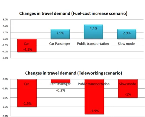
Before describing the traffic safety impact of the two TDM scenarios, it would be beneficial to have a look at the changes made to the more traffic-related attributes playing a role in the whole chain. As described before, increasing fuel-related costs will affect and increase the total travel expenses of motor vehicle trips or motivating teleworking will let a certain percentage of working population to work from home. In the case of fuel-cost increase scenario, people will start comparing the relative costs of travelling and may consider a shift to other available transportation modes. For instance, short-distance trips can be substituted by public transportation (e.g. bus or tram) or slow mode (i.e. biking or walking) or long-distance trips may shift towards public transportation (e.g. train) or be substituted by carpooling. In the case of teleworking scenario, many trips are cancelled and teleworkers are staying at home. However, it is possible that the remaining scheduled trips (except of work related trips) of teleworkers still need to be performed. These trips are often short-distance trips and are usually carried out by public transportation (e.g. bus or tram) or slow mode (i.e. biking or walking).

Comparing OD matrices derived from the activity-based model for the null and both the fuel-cost increase and the teleworking scenarios enables us to perceive any changes in NOTs for different modes and will also allow us to figure out if any mode shift has occurred. Changes in NOTs are shown in Figure 2. The results of these comparisons revealed that the fuel-cost increase scenario has a mixed effect in changing the NOTs, while the teleworking scenario reduces the NOTs for all types of travel mode.

(12)

11

Figure 2: Changes in travel demand after implementing the two TDM scenarios

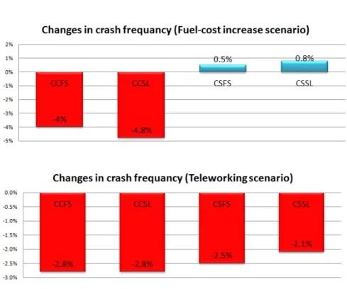
Predictably, in the fuel-cost increase scenario the total number of predicted “Car-Car” crashes decreases compared to the null scenario. This is due to reduced car exposure as the main predictor of these types of crashes. On the contrary and as a result of an increase in Slowmode NOTs, for “Car-Slowmode” crashes a slight increase is observed for both “fatal + severe injury” and “slight injury” crashes. Furthermore, in the teleworking scenario and as a result of reduced exposure for both car and Slowmode NOTs, the total predicted NOCs for all types of crashes decrease compared to the null scenario. Figure 3 depicts changes in NOCs for all types of crashes and for both the fuel-cost increase and the teleworking scenarios.

(13)

12

Figure 3: Changes in predicted crash frequency after implementing the two TDM scenarios To have a better insight into the distributional changes in NOCs, Figure 4 represents the violin plots of changes in NOCs after the fuel-cost increase and the teleworking scenarios implementation. The violin plot is a synergistic combination of the box plot and the density trace (Hintze and Nelson, 1998). These plots retain much of the information of box plots (except for the individual outliers), besides providing information about the distributional characteristics of the data. In these plots, the wider the violin, the more data points are associated to that value. Moreover, the white dots indicate the median; black boxes show the upper and lower quartile and the vertical black lines denote the upper and lower whiskers.

(14)

13

Figure 4: Violin plots of changes in crash occurrence after TDM scenarios implementation In the development of “Car-Slowmode” models, both car and Slowmode-related exposure variables were used. Following the implementation of the fuel-cost increase scenario and as a result of mode shift, the number of car trips decreased whereas the number of Slowmode trips increased. However, these mode shifts are not always similar in all TAZs; i.e. more urbanized areas have a higher number of mode shifts and consequently more Slowmode-related crashes are predicted to occur in these areas.

Following the implementation of the teleworking scenario, the total number of car and Slowmode trips decreased. However, these changes are not always similar in all TAZs. In fact, in more urbanized areas, the NOTs reduces more heavily and, therefore, also the NOCs reduces more rapidly in these areas. This can be explained by the fact that most of the commuters commute to urbanized areas.

(15)

14

5 CONCLUSIONS AND DISCUSSION

In this study, the traffic safety impacts of two TDM scenarios (i.e. the fuel-cost increase and the teleworking scenario) are evaluated. To this end, ZCPMs are coupled with the activity-based model, FEATHERS. Based on the results of the analyses, the following conclusions can be drawn:

Activity-based transportation models provide an adequate range of in-depth information about individuals’ travel behavior to realistically simulate and evaluate TDM strategies. The main advantage of these models is that the impact of applying a TDM strategy will be accounted for, for each individual, throughout a decision making process instead of applying the scenario on a general population level. Activity-based models, therefore, provide more reliable travel information since, unlike traditional models, TDM strategies are inherently accounted for in these models. Activity-based models follow a disaggregate modeling approach and as such, allow for a more detailed analysis of the reduction of travel demand due to the implementation of TDM scenarios.

In crash analysis, predictor variables are often found to be spatially heterogeneous especially when the study area is large enough to cover different traffic volume, urbanization and socio-demographic patterns. The results of the analysis confirm the presence of spatial correlation of dependent and different explanatory variables which are used in developing crash prediction models. This was examined by computing Moran’s I statistics for the dependent and selected explanatory variables. The results reveal the necessity of considering spatial correlation when developing crash prediction models.

The results of the comparison analysis revealed that both of the TDM scenarios has many impacts such as mode shift and reductions of total travel demand, total crash occurrence, VKT and VHT. On the whole, there is a reduction of on average 105,000 and 167,000 daily trips (all types of modes) and a reduction of nearly 5 and 1.4 billion VKT by cars per year as a result of the fuel-cost increase and the teleworking scenario, respectively.

When considering the changes in the NOCs at the TAZ level, it was found that the maximum reduction of “Car-Car” crashes and the maximum increase of “Car-Slowmode” crashes were both observed in urban areas (i.e. cities) after implementing the fuel-cost increase scenario. It can be concluded that in cities, in contrast to other areas, there is a higher likelihood of finding an alternative mode for cars. In contrast, the TAZs in less urbanized regions and the TAZs nearby the borders usually lack good public transportation services. Therefore, it is expected that we will not see many trips shift from cars to other modes in less urbanized areas and consequently there is a more stable traffic safety situation in these TAZs despite conducting the fuel-cost increase scenario. For the teleworking scenario, it turns out that especially urbanized areas (cities) benefit most from a general reduction of “Car-Car” and “Car-Slowmode” crashes. This can be due to the fact that most of businesses that allow their employees to telework are generally located in cities.

In summary, adopting a fuel-cost increase policy can generally be recommended from the road safety point of view and due to its positive impacts on crash frequency reduction. However, the slight negative effect on the traffic safety level of vulnerable road users requires special attention. These negative impacts can be diminished by improving cycle paths infrastructure, improving public transportation efficiency, etc. Moreover, it should be noticed that these positive impacts are fully realizable, only in the short term. In the long run and due to the shift in the composition of the vehicle fleet or changes in the location of

(16)

15

businesses and/or the location choice for living, these positive impacts might erode. Hence, fuel-cost increase strategies should be considered as medium term effective TDM policies, with respect to their road safety impacts.

Crashes are known to be a function of two components; exposure and risk. It is therefore likely that a fuel price increase will impact people’s driving behavior and their speed choice; i.e. drivers might try to reduce their fuel consumption by driving more slowly. As a result, it can be assumed that the risk component will also decrease after the fuel-cost increase scenario implementation. In this study however, only the changes in the exposure component were taken into account, whereas the risk component was assumed to be constant. This might be a limitation of this study. If we were to include the risk component in this study as well, however, the traffic safety benefits might be expected to be even larger than predicted in this study.

Due to the observed mixed effects of TDM scenarios on the safety levels of different road users, decision makers and road engineers are strongly recommended to make a distinction between different road users when carrying our any safety assessment. Moreover, combined policies might complement each other and accordingly, desired safety benefits might be realized with more confidence. Another policy related issue that needs further exploration is the safety assessment of other TDM policies; i.e. separately assessment of an aging population, a public transportation level-of-service improvement and their combination with the studied policies in this research are on the list of the future research agenda.

Moreover, the real power of activity-based models has not yet been fully incorporated. In this study, the methodology relied on the aggregate daily traffic information. Activity-based models are however capable of providing disaggregate travel characteristics by differentiating between many household and person characteristics like gender, age, number of cars, etc. Hence, different types of disaggregation based on time of day, age, gender and motive are on the list of potential future research in order to take full advantage of the output of activity-based models.

REFERENCES

Abdel-Aty, M., Siddiqui, C., Huang, H., 2011a. Zonal Level Safety Evaluation Incorporating Trip Generation Effects. Presented at the Transportation Research Board (TRB) 90th Annual Meeting, Washington D.C. USA.

Abdel-Aty, M., Siddiqui, C., Huang, H., 2011b. Integrating Trip and Roadway Characteristics in Managing Safety at Traffic Analysis Zones. Presented at the Transportation Research Board (TRB) 90th Annual Meeting, Washington D.C. USA. Aguero-Valverde, J., Jovanis, P.P., 2006. Spatial analysis of fatal and injury crashes in

Pennsylvania. Accident Analysis & Prevention 38, 618–625.

Aguero-Valverde, J., Jovanis, P.P., 2008. Analysis of Road Crash Frequency with Spatial Models. Transportation Research Record: Journal of the Transportation Research Board 2061, 55–63.

Amoros, E., Martin, J.L., Laumon, B., 2003. Comparison of road crashes incidence and severity between some French counties. Accident Analysis & Prevention 35, 537–547.

(17)

16

An, M., Casper, C., Wu, W., 2011. Using Travel Demand Model and Zonal Safety Planning Model for Safety Benefit Estimation in Project Evaluation. Presented at the

Transportation Research Board (TRB) 90th Annual Meeting, Washington D.C. USA. Arentze, T.A., Timmermans, H.J.P., 2004. ALBATROSS – Version 2.0 – A learning based

transportation oriented simulation system. EIRASS (European Institute of Retailing and Services Studies).

Chen, V.Y.-J., Yang, T.-C., 2012. SAS macro programs for geographically weighted generalized linear modeling with spatial point data: Applications to health research. Computer Methods and Programs in Biomedicine 107, 262–273.

Chi, G., Cosby, A.G., Quddus, M.A., Gilbert, P.A., Levinson, D., 2010. Gasoline prices and traffic safety in Mississippi. Journal of Safety Research 41, 493–500.

Choo, S., Mokhtarian, P.L., 2007. Telecommunications and travel demand and supply: Aggregate structural equation models for the US. Transportation Research Part A: Policy and Practice 41, 4–18.

Choo, S., Mokhtarian, P.L., Salomon, I., 2005. Does telecommuting reduce vehicle-miles traveled? An aggregate time series analysis for the U.S. Transportation 32, 37–64. Davidson, W., Donnelly, R., Vovsha, P., Freedman, J., Ruegg, S., Hicks, J., Castiglione, J.,

Picado, R., 2007. Synthesis of first practices and operational research approaches in activity-based travel demand modeling. Transportation Research Part A: Policy and Practice 41, 464–488.

De Guevara, F.L.D., Washington, S., Oh, J., 2004. Forecasting Crashes at the Planning Level: Simultaneous Negative Binomial Crash Model Applied in Tucson, Arizona.

Transportation Research Record: Journal of the Transportation Research Board 1897, 191–199.

Dissanayake, D., Morikawa, T., 2008. Impact assessment of satellite centre-based

telecommuting on travel and air quality in developing countries by exploring the link between travel behaviour and urban form. Transportation Research Part A: Policy and Practice 42, 883–894.

Flahaut, B., 2004. Impact of infrastructure and local environment on road unsafety: Logistic modeling with spatial autocorrelation. Accident Analysis & Prevention 36, 1055–1066. Fotheringham, A.S., Brunsdon, C., Charlton, M., 2002. Geographically Weighted Regression

the analysis of spatially varying relationships. John Wiley & Sons Ltd, West Sussex, England.

Goodwin, P., Dargay, J., Hanly, M., 2004. Elasticities of Road Traffic and Fuel Consumption with Respect to Price and Income: A Review. Transport Reviews 24, 275–292.

(18)

17

Grabowski, D.C., Morrisey, M.A., 2004. Gasoline Prices and Motor Vehicle Fatalities. Journal of Policy Analysis and Management 23, 575–593.

Guo, F., Wang, X., Abdel-Aty, M., 2010. Modeling signalized intersection safety with corridor-level spatial correlations. Accident Analysis & Prevention 42, 84–92.

Hadayeghi, A., Shalaby, A., Persaud, B., 2003. Macrolevel Accident Prediction Models for Evaluating Safety of Urban Transportation Systems. Transportation Research Record: Journal of the Transportation Research Board 1840, 87–95.

Hadayeghi, A., Shalaby, A., Persaud, B., 2007. Safety Prediction Models: Proactive Tool for Safety Evaluation in Urban Transportation Planning Applications. Transportation Research Record: Journal of the Transportation Research Board 2019, 225–236. Hadayeghi, A., Shalaby, A., Persaud, B., 2010. Development of Planning-Level

Transportation Safety Models using Full Bayesian Semiparametric Additive Techniques. Journal of Transportation Safety & Security 2, 45–68.

Hadayeghi, A., Shalaby, A.S., Persaud, B.N., Cheung, C., 2006. Temporal transferability and updating of zonal level accident prediction models. Accident Analysis & Prevention 38, 579–589.

Hakkert, A.S., Braimaister, L., 2002. The uses of exposure and risk in road safety studies (No. R-2002-12). SWOV Institute for Road Safety Research, Leidschendam, The Netherlands.

Henderson, D.K., Mokhtarian, P.L., 1996. Impacts of center-based telecommuting on travel and emissions: Analysis of the Puget Sound Demonstration Project. Transportation Research Part D: Transport and Environment 1, 29–45.

Hintze, J.L., Nelson, R.D., 1998. Violin Plots: A Box Plot-Density Trace Synergism. The American Statistician 52, 181–184.

Huang, H., Abdel-Aty, M., Darwiche, A., 2010. County-Level Crash Risk Analysis in Florida. Transportation Research Record: Journal of the Transportation Research Board 2148, 27–37.

Janssens, D., Wets, G., Timmermans, H.J.P., Arentze, T.A., 2007. Modelling Short-Term Dynamics in Activity-Travel Patterns: Conceptual Framework of the Feathers Model. Presented at the 11th World Conference on Transport Research, Berkeley CA, USA. Kochan, B., Bellemans, T., Cools, M., Janssens, D., Wets, G., 2011. An estimation of total

vehicle travel reduction in the case of telecommuting: Detailed analyses using an activity-based modeling approach. Presented at the European Transportation Conference, Glasgow, Scotland, UK.

(19)

18

Koenig, B.E., Henderson, D.K., Mokhtarian, P.L., 1996. The travel and emissions impacts of telecommuting for the state of California Telecommuting Pilot Project. Transportation Research Part C: Emerging Technologies 4, 13–32.

Lee, J., Wong, D.W.S., 2001. Statistical analysis with ArcView GIS. John Wiley & Sons, Inc., United States of America.

Levine, N., Kim, K.E., Nitz, L.H., 1995. Spatial analysis of Honolulu motor vehicle crashes: II. Zonal generators. Accident Analysis & Prevention 27, 675–685.

Litman, T., 2003. The Online TDM Encyclopedia: mobility management information gateway. Transport Policy 10, 245–249.

Litman, T., 2006. Mobility Management Traffic Safety Impacts. Presented at the

Transportation Research Board (TRB) 85th Annual Meeting, Washington D.C. USA. Litman, T., 2010. Changing Vehicle Travel Price Sensitivities: The Rebounding Rebound

Effect.

Litman, T., Fitzroy, S., 2012. Safe Travels: Evaluating Mobility Management Traffic Safety Impacts. Victoria Transport Policy Institute.

Lord, D., Mannering, F., 2010. The statistical analysis of crash-frequency data: A review and assessment of methodological alternatives. Transportation Research Part A: Policy and Practice 44, 291–305.

Lovegrove, G., Sayed, T., 2007. Macrolevel Collision Prediction Models to Enhance Traditional Reactive Road Safety Improvement Programs. Transportation Research Record: Journal of the Transportation Research Board 2019, 65–73.

Lovegrove, G.R., 2005. Community-Based, Macro-Level Collision Prediction Models (Doctoral thesis).

Lovegrove, G.R., Litman, T., 2008. Using Macro-Level Collision Prediction Models to Evaluate the Road Safety Effects of Mobility Management Strategies: New Empirical Tools to Promote Sustainable Development. Presented at the Transportation Research Board (TRB) 87th Annual Meeting, Washington D.C. USA.

Lovegrove, G.R., Sayed, T., 2006. Macro-level collision prediction models for evaluating neighbourhood traffic safety. Canadian Journal of Civil Engineering 33, 609–621. Miaou, S.-P., Song, J.J., Mallick, B.K., 2003. Roadway Traffic Crash Mapping: A

Space-Time Modeling Approach. Journal of Transportation and Statistics 6, 33–57.

Mokhtarian, P.L., Varma, K.V., 1998. The trade-off between trips and distance traveled in analyzing the emissions impacts of center-based telecommuting. Transportation Research Part D: Transport and Environment 3, 419–428.

(20)

19

Naderan, A., Shahi, J., 2010. Aggregate crash prediction models: Introducing crash generation concept. Accident Analysis & Prevention 42, 339–346.

Nilles, J.M., 1996. What does telework really do to us? World Transport Policy & Practice 2, 15–23.

Noland, R.B., Oh, L., 2004. The effect of infrastructure and demographic change on traffic-related fatalities and crashes: a case study of Illinois county-level data. Accident Analysis & Prevention 36, 525–532.

Noland, R.B., Quddus, M.A., 2004. A spatially disaggregate analysis of road casualties in England. Accident Analysis & Prevention 36, 973–984.

Pirdavani, A., Brijs, T., Bellemans, T., Kochan, B., Wets, G., 2012. Developing Zonal Crash Prediction Models with a Focus on Application of Different Exposure Measures. Transportation Research Record: Journal of the Transportation Research Board. Pirdavani, A., Brijs, T., Bellemans, T., Kochan, B., Wets, G., 2013. Evaluating the road

safety effects of a fuel cost increase measure by means of zonal crash prediction modeling. Accident Analysis & Prevention 50, 186–195.

Quddus, M.A., 2008. Modelling area-wide count outcomes with spatial correlation and heterogeneity: An analysis of London crash data. Accident Analysis & Prevention 40, 1486–1497.

Siddiqui, C., Abdel-Aty, M., Choi, K., 2012. Macroscopic spatial analysis of pedestrian and bicycle crashes. Accident Analysis & Prevention 45, 382–391.

Tarko, A., Inerowicz, M., Ramos, J., Li, W., 2008. Tool with Road-Level Crash Prediction for Transportation Safety Planning. Transportation Research Record: Journal of the Transportation Research Board 2083, 16–25.

Vovsha, P., Bradley, M., 2006. Advanced Activity-Based Models in Context of Planning Decisions. Transportation Research Record: Journal of the Transportation Research Board 1981, 34–41.

VTPI, 2012. VTPI. Online TDM Encyclopedia, Victoria Transport Policy Institute.

Vu, S.T., Vandebona, U., 2007. Telecommuting and Its Impacts on Vehicle-km Travelled. Presented at the International Congress on Modelling and Simulation, University of Canterbury, Christchurch, New Zealand.

Wang, C., Quddus, M.A., Ison, S.G., 2009. Impact of traffic congestion on road accidents: A spatial analysis of the M25 motorway in England. Accident Analysis & Prevention 41, 798–808.

Wang, X., Abdel-Aty, M., 2006. Temporal and spatial analyses of rear-end crashes at signalized intersections. Accident Analysis & Prevention 38, 1137–1150.

(21)

20

Wier, M., Weintraub, J., Humphreys, E.H., Seto, E., Bhatia, R., 2009. An area-level model of vehicle-pedestrian injury collisions with implications for land use and transportation planning. Accident Analysis & Prevention 41, 137–145.