Levels of measurement and statistical analyses
Matt N. Williams
School of Psychology, Massey University
Most researchers and students in psychology learn of S. S. Stevens’ scales or “levels” of measurement (nominal, ordinal, interval, and ratio), and of his rules setting out which statistical analyses are admissible with each measurement level. Many are nevertheless left confused about the basis of these rules, and whether they should be rigidly followed. In this article, I attempt to provide an accessible explanation of the measurement-theo-retic concerns that led Stevens to argue that certain types of analyses are inappropriate with data of particular levels of measurement. I explain how these measurement-theo-retic concerns are distinct from the statistical assumptions underlying data analyses, which rarely include assumptions about levels of measurement. The level of measure-ment of observations can nevertheless have important implications for statistical as-sumptions. I conclude that researchers may find it more useful to critically investigate the plausibility of the statistical assumptions underlying analyses than to limit themselves to the set of analyses that Stevens believed to be admissible with data of a given level of measurement.
Keywords: Levels of measurement, measurement theory, ordinal, statistical analysis.
Introduction
Most students and researchers in psychology learn of a division of measurement into four scales: nominal, ordinal, interval, and ratio. This taxonomy was created by the psychophysicist S. S. Stevens (1946). Stevens wrote his article in response to a long-running debate within a committee of the Brit-ish Association for the Advancement of Science which had been formed in order to consider the question of whether it is possible to measure “sen-sory events” (i.e., sensations and other psychological attributes; see Ferguson et al., 1940). The committee was partly made up of physical scientists, many of whom believed that the numeric recordings taking
1 For example, the term “scale” is often used to refer to
specific psychological tests or measuring devices (e.g., the “hospital anxiety and depression scale”; Zigmond & Snaith, 1983). It is also often used to refer to formats for
place in psychology (specifically psychophysics) did not constitute measurement as the term is usually understood in the natural sciences (i.e., as the esti-mation of the ratio of a magnitude of an attribute to some unit of measurement; see Michell, 1999). Ste-vens attempted to resolve this debate by suggesting that it is best to define measurement very broadly as “the assignment of numerals to objects or events ac-cording to rules” (Stevens, 1946, p. 677), but then di-vide measurements into four different “scales”. These are now often referred to as “levels” of meas-urement, and that is the terminology I will predom-inantly use in this paper, as the term “scales” has other competing usages within psychometrics1.
Ac-cording to Stevens’ definition of measurement, vir-tually any research discipline can claim to achieve measurement, although not all may achieve interval
collecting responses (e.g., “a four-point rating scale”). These contemporary usages are quite different from Ste-vens “scales of measurement” and therefore the term “levels of measurement” is somewhat less ambiguous.
or ratio measurement. He went on to argue that the level with which an attribute has been measured de-termines which statistical analyses are permissible (or “admissible”) with the resulting data.
Stevens’ definition and taxonomy of measure-ment has been extremely influential. Although I have not conducted a rigorous evaluation, it appears to be covered in the vast majority of research methods textbooks aimed at students in the social sciences (e.g., Cozby & Bates, 2015; Heiman, 2001; Judd et al., 1991; McBurney, 1994; Neuman, 2000; Price, 2012; Ray, 2000; Sullivan, 2001). Stevens’ taxonomy is also often used as the basis for heuristics indicating which statistical analyses should be used in particu-lar scenarios (see for example Cozby & Bates, 2015).
However, the fame and influence of Stevens’ tax-onomy is something of an anomaly in that it forms part of an area of inquiry (measurement theory) which is rarely covered in introductory texts on re-search methods2. Measurement theories are
theo-ries directed at foundational questions about the nature of measurement. For example, what does it mean to “measure” something? What kinds of attrib-utes can and cannot be measured? Under what con-ditions can numbers be used to express relations amongst objects? Measurement theory can arguably be regarded as a branch of philosophy (see Tal, 2017), albeit one that has heavily mathematical features. The measurement theory literature contains several excellent resources pertaining to the topic of admis-sibility of statistical analyses (e.g., Hand, 1996; Luce et al., 1990; Michell, 1986; Suppes & Zinnes, 1962), but this literature is often written for an audience of readers who have a reasonably strong mathematical background, and can be quite dense and challeng-ing. This means that, while many students and re-searchers are exposed to Stevens’ rules about ad-missible statistics, few are likely to understand the
basis of these rules. This can often lead to significant
confusion about important applied questions: For example, is it acceptable to compute “parametric” statistics using observations collected with a Likert scale?
2 By way of example, the well-known textbook
“Psycho-logical Testing: Principles, Applications, & Issues” by Kaplan and Saccuzzo (2018) covers Stevens’ taxonomy and rules about permissible statistics (albeit without at-tribution to Stevens), but does not mention any of the
In this article, therefore, I attempt to provide an accessible description of the rationale for Stevens’ rules about admissible statistics. I also describe some major objections to Stevens’ rules, and explain how Stevens’ measurement-theoretic concerns are different from the statistical assumptions underly-ing statistical analyses—although there exist im-portant connections between the two. I close with conclusions and recommendations for practice.
Stevens’ Taxonomy of Measurement
Stevens’ definition and taxonomy of measure-ment was inspired by two theories of measuremeasure-ment: Representationalism, especially as expressed by Campbell (1920), and operationalism, especially as expressed by Bridgman (1927)3. Operationalism (see
Bridgman, 1927; Chang, 2009) holds that an attribute is fully synonymous with the operations used to measure it: That if I say I have measured depression using score on the Beck Depression Inventory (BDI), then when I speak of a participant’s level of depres-sion, I mean nothing more or less than the score the participant received on the BDI. Stevens’ definition of measurement— as “the assignment of numerals to objects or events according to rules” (Stevens, 1946, p. 677)—is based on operationalism. In contrast to operationalism, representationalism argues that measurement starts with a set of observable empir-ical relations amongst objects. The objects of meas-urement could literally be inanimate objects (e.g., rocks), but they could also be people (e.g., partici-pants in a research study). To a representationalist,
measurement consists of transferring the knowledge
obtained about the empirical relations amongst ob-jects (e.g., that granite is harder than sandstone) into numbers which encode the information obtained about these empirical relations (see Krantz et al., 1971; Michell, 2007).
Stevens suggested that levels of measurement are distinguished by whether we have “empirical op-erations” (p. 677) for determining relations (equality, rank-ordering, equality of differences, and equality of ratios). This is an idea that appears to have been
measurement theories discussed in this section (opera-tionalism, representa(opera-tionalism, and the classical theory of measurement).
3 See McGrane (2015) for a discussion of these competing
influenced by representationalism (representation-alism being a theory that concerns the use of num-bers to represent information about empirical rela-tions). Nevertheless, an influence of operationalism is apparent here also: To Stevens, the level of meas-urement of a set of observations depended on whether an empirical operation for determining equality, rank-ordering, equality of differences and/or equality of ratios was applied (regardless of the degree to which the empirical operation pro-duced valid determinations of these empirical rela-tions).
While Stevens’ definition and taxonomy of meas-urement incorporates both representational and operationalist influences, there is a third theory of measurement that he did not incorporate: The clas-sical theory of measurement. This theory of meas-urement has been the implicit theory of measure-ment in the physical sciences since classical antiq-uity (Michell, 1999). The classical theory of measure-ment states that to measure an attribute is to esti-mate the ratio of the magnitude of an attribute to a unit of the same attribute. For example, to say that we have measured a person’s height as 185cm means that we have estimated that the person’s height is 185 times that of one centimetre (the unit). The clas-sical theory of measurement suggests that only some attributes—quantitative attributes—have a structure such that their magnitudes stand in ratios to one another. A set of axioms demonstrating what conditions need to be met for an attribute to be quantitative were determined by the German math-ematician Otto Hölder (1901; for an English transla-tion see Michell & Ernst, 1996). Because the focus of this article is on Stevens’ arguments, I will not cover the classical theory of measurement further in this article, but excellent introductions can be found in Michell (1986, 1999, 2012). It may suffice at this point to note that from a classical perspective, Stevens’ “nominal” and “ordinal” levels do not constitute measurement at all.
Stevens defined his four scales or levels of meas-urement as follows.
Nominal
According to Stevens (1946), nominal measure-ment is produced when we have an empirical oper-ation that allows us to determine that some objects are equivalent with respect to some attribute, while
other objects are noticeably different. For example, imagine we have a group of university students, and via the empirical operation of looking up their aca-demic records we can determine that some of the students are psychology majors while some are business majors. If we wished to compare the psy-chology students and the business students with re-spect to some other attribute, we might record in-formation about the participants and their majors in a dataset. For the sake of convenience, we might do so by recording their majors numerically. Specifi-cally, we might enter a 0 in a “Major” column in the dataset for each of the psychology students, and a 1 for each of the business students. In doing so, ac-cording to Stevens, we would have accomplished nominal measurement. Importantly, there are many coding rules that would work just as effectively at conveying the information we have about partici-pants’ majors. For example, we could just as well use 1 to indicate a psychology student and 0 to indicate a business student, or -10 to indicate a psychology student and 437.3745 to indicate a business student. As long as students’ majors are recorded by assign-ing the psychology students one fixed number and business students another, any two numbers would work just as well at conveying what we have ob-served about the students.
Ordinal
Ordinal measurement is produced when we have an empirical operation that allows us to determine that some objects are greater or lesser than others with respect to some attribute. Imagine, for exam-ple, that we are interested in the attribute
satisfac-tion with life. We perform the empirical operasatisfac-tion of
asking three participants (Hakim, Jeff, and Sarah) to respond to the question “In general, how satisfied are you with your life?” (see Cheung & Lucas, 2014, p. 2811), with response options of very dissatisfied, moderately dissatisfied, moderately satisfied, and very satisfied. We discover that Hakim indicates that he is very satisfied with life, while Jeff is moderately satisfied, and Sarah is moderately dissatisfied. We have thus performed an empirical operation that al-lows us to determine whether each of these partici-pants has more or less life satisfaction than another.
If we are to record this information numerically, there are many possible coding rules that could
con-vey the information collected about the life satisfac-tion of our participants, but there is a restricsatisfac-tion: The number assigned to Hakim must be higher than the number assigned to Jeff, which must be higher again than that assigned to Sarah. Any such coding rule will record what we have observed: That Hakim has the highest level of life satisfaction, followed by Jeff, followed by Sarah. So, we could assign Hakim a life satisfaction score of 3, Jeff a score of 2, and Sarah a score of 1. Or we could also assign Hakim a score of 1234, Jeff a score of 6, and Sarah a score of 0.45. Either of these two coding rules records the ob-served ordering Hakim > Jeff > Sarah, and from Ste-vens’ perspective each would be just as adequate as the other. However, we could not assign Hakim a score of 3, Jeff a score of 1, and Sarah a score of 2; this would imply that Sarah has higher life satisfac-tion than Jeff, which conflicts with the empirical in-formation we have collected. Formally, any coding system within the class of monotonic transfor-mations will equivalently convey the information that we have about the participants. In other words, if we have assigned numeric scores to the partici-pants such that Hakim > Jeff > Sarah, then we can transform those numeric scores in any way provided that the order of the scores (Hakim > Jeff > Sarah) remains the same.
Interval
Interval measurement is produced when, in ad-dition to having an empirical operation that allows us to observe that some objects are greater or less than others with respect to some attribute, we have an empirical operation that allows us to determine whether the difference between a pair of objects is greater than, less than, or the same as the difference between another pair of objects. The classic exam-ple of an interval scale is temperature when meas-ured via a mercury thermometer (i.e., a narrow glass tube containing mercury, with a bulb at the bottom, held upright). If we place the thermometer inside a fridge, we can see that the mercury level will be 4 The fact that this assumption is necessary points to the
important role theory can have in measurements; for a sophisticated discussion in the context of thermometers and the measurement of temperature, see Sherry (2011).
5 In fact, it is also possible to produce interval
measure-ment based only on observations about order and equal-ity of differences along with some other conditions; see
lower than if we placed the thermometer in a living room. It will be lower again if we place the thermom-eter in a freezer. If we are willing to assume that mercury expands with increasing temperature, this empirical observation allows us to determine that, with respect to temperature, living room > fridge >
freezer.
This observation alone would be a purely ordinal one. However, we can also use a ruler to measure the highest point reached by the mercury in each lo-cation. By this method, we can determine whether the distance the mercury expands by when moved from the freezer to the fridge is more, the same, or less than the distance it expands by when moved from the fridge to the living room. If we are willing to assume that the relationship between tempera-ture and the height of the mercury in the thermom-eter is linear within the range of temperatures ob-served4, then we can also empirically compare dif-ferences between observations. For example, we
might attach a ruler to our tube of mercury, and ob-serve that the difference in the height of the mer-cury between the living room and the fridge is 5 mm, while the difference between the height of the mer-cury in the fridge and in the freezer is 10 mm. Given our assumption of linear expansion of mercury with temperature, this implies that the difference in tem-perature between the fridge and the living room is twice5 the difference in temperature between the
freezer and the fridge. Because we have an empirical operation that allows us to compare differences in temperature, we have achieved interval measure-ment.
The information we have collected about the temperature of the fridge, the freezer, and the living room can be recorded via a variety of coding rules, but there is now an additional restriction: Not only must the coding rule preserve the observed order-ing livorder-ing room > fridge > freezer, but the difference between the number we assign to the fridge and the one we assign to the freezer must be twice the dif-ference between the number we assign to the living
Suppes and Zinnes’ (1962) description of infinite differ-ence systems. For the sake of simplicity and brevity I have focused here on the simpler scenario of observa-tions about ratios of differences.
room and the fridge. We could record the freezer as having a temperature of 0, the fridge a temperature of 2, and the living room a temperature of 3. Or we could record the freezer as having a temperature of 5, the fridge a temperature of 15, and the living room a temperature of 20. But we should not record the freezer as having a temperature of 0, the fridge a temperature of 1, and the living room a temperature of 3; this would imply that the difference in temper-ature between the living room and the fridge is greater than that between the fridge and the freezer. More formally, if we have a coding rule that records the information we have collected about these temperature, we can apply any linear trans-formation to it (e.g., by multiplying the existing val-ues by some number and/or adding a constant) while still adequately representing the information we have collected about the temperatures.
It is worth emphasising here that it is the fact we can empirically compare differences between tem-peratures that implies that we have achieved inter-val measurement. The argument has sometimes been made (e.g., Carifio & Perla, 2008) that while the responses to a rating scale item (as in the earlier ex-ample for life satisfaction) are ordinal in nature, a score created by summing the responses to multiple items is interval. This argument confuses the issue of level of measurement with that of the distribution of a variable. The act of summing ordinal observa-tions may increase the degree to which the distribu-tion of scores approximates a normal distribudistribu-tion but does not transform these observations from or-dinal to interval (because it does not provide an op-eration for determining equality of differences).
Ratio
Imagine, now, that we wish to compare the lengths of two objects: A pen and a rolling pin. By placing these objects side-by-side we can quickly establish that the rolling pin is the longer. Let us as-sume that we have several of the same model of pen, each of identical length. Now imagine we lay three 6 For the sake of simplicity, the situation I describe here
is one where the length of one of the objects is exactly divisible by the length of the other. In reality, it might be the case that the rolling pin is slightly longer than three pens, such that I can conclude only that the ratio of the length of the rolling pin to the pen falls in the interval [3, 4]. But we could obtain a more precise estimate of the
of these pens end to end with one another and ob-serve that the rolling pin appears to be equal in length to the three pens6. In other words, we have
observed that the ratio of the length of the rolling pin to that of the pen is 3. Therefore, we have achieved ratio measurement.
Once again, these observations can be recorded numerically, but our choice of coding rule is now very restricted: Whatever number we assigned as the length of the rolling pin must be three times the number assigned to the pen. So we might record the pen as having a length of 1 and the rolling pin a length of 3, or the pen a length of 0.5 and the rolling pin a length of 1.5, but we could not assign the pen a length of 1 and the rolling pin a length of 2. More formally, if we have applied a coding rule that records the information we have collected about the ratios of the lengths of the objects, then the only transformation we can apply to the numeric values is multiplying them by some constant.
Stevens’ “Admissible Statistics”
The connection Stevens drew between levels of measurement and statistical analysis was this: Given observations pertaining to a set of objects, there are a variety of coding rules that one could use to en-code the information held about the empirical rela-tions amongst objects. Furthermore, if we consider the four levels of measurement on a hierarchy from ratio at the top to nominal at the bottom, the lower levels of measurement offer a much more diverse range of coding rules from which one can arbitrarily select. Statistical analyses, however, may produce different results depending on which coding rule is used, so we should only use statistical analyses that produce invariant results across the class of coding rules that are permissible for the data we have col-lected.
By way of example, let’s return to our measure-ments of life satisfaction from three participants: Hakim (who was very satisfied with his life), Jeff
length of the rolling pin if we had a “standard sequence” of many replicates of the same short length. A ruler measured in millimetres, for example, just represents a sequence of identical one-millimetre lengths laid end to end. For a more rigorous treatment of this topic, see Krantz et al. (1971)
(moderately satisfied), and Sarah (moderately dis-satisfied). Imagine now that we recruit a fourth par-ticipant, Ming, who transpires to be very dissatisfied with life. We wish to use these four participants to test the hypothesis that owning a pet is associated with increased life satisfaction. We ask our partici-pants whether they each own a pet; it turns out that Hakim and Jeff do, while Sarah and Ming do not. We can now proceed to comparing the life satisfaction of these two groups of participants. Recall, though, that we have only ordinal observations of life satis-faction, and can apply any coding rule to our obser-vations that preserves the ordering Hakim > Jeff >
Sarah > Ming. The outcomes of two such coding
rules are displayed in Table 1. Table 1
Example Life Satisfaction Data
Life satisfaction
Partici-pant Owns pet? Qualitative response rule one Coding rule two Coding
Hakim Yes Very
satisfied
4 1002
Jeff Yes Moderately
satisfied 3 1000 Mean (SD) 3.5 (0.71) 1001 (1.41) Sarah No Moderately dissatisfied 2 1 Ming No Very dissatisfied 1 0 Mean (SD) 1.5 (0.71) 0.5 (0.71) Note. Coding rule one: Very dissatisfied = 1, moderately dissatisfied = 2, moderately satisfied = 3, very satisfied = 4. Coding rule two: Very dissatisfied = 0, moderately dissat-isfied = 1, moderately satdissat-isfied = 1000, very satdissat-isfied = 1002.
If we applied a Student’s t test to compare the mean life satisfaction ratings of the two groups (pet owners, non- pet owners), we would discover that the results differ depending on which coding rule we use. For coding rule one, the mean difference in life satisfaction between the pet owners and the non-pet owners is 2, and this difference is not statistically significant, t(2) = 2.83, p = .106. But for coding rule two, the mean difference in life satisfaction is 1000.5, and this difference is statistically significant,
t(2) = 894.87, p < .001. Thus, it seems that the
out-come of the Student’s t test varies across these two equally permissible coding rules, which does not seem like a satisfactory state of affairs. On the other
hand, if we compare the two samples using a Mann-Whitney U test, the resulting p value is identical across the two coding rules (being p = .33). This is the case for the simple reason that the Mann-Whit-ney U is calculated using the ranks of the observa-tions rather than their numeric coded values. As such, we might argue that the Mann-Whitney U sta-tistic and its associated p value is invariant across the class of permissible transformations with ordi-nal data, whereas the Student’s t test is not, and that as such the Mann-Whitney U is the more appropri-ate test.
Stevens went on to set out a list of statistical analyses that he believed would produce invariant results for variables of each level of measurement. For example, he suggested that a median is admissi-ble as a measure of central tendency for an ordinal variable, since the case (or pair of cases) that falls at the median will always be the same across any mon-otonic transformation of the variable, even if the nu-meric value of the median will not. On the other hand, he suggested that a mean is not an admissible measure of central tendency with ordinal data, be-cause both the actual value of the mean and the case to which it most closely corresponds will both differ across monotonic transformations of the observa-tions. In noting these distinctions, it is clear there exists a degree of ambiguity about what constitutes “invariance”. Michell (1986) and Luce et al. (1990) provide more formal examination of the type of in-variance that is implied by Stevens’ arguments.
Parametric and Non-Parametric Statistics
It is common for authors to claim that the issue of admissibility raised by Stevens implies that
para-metric statistical analyses should only be used with
interval or ratio data (e.g., Jamieson, 2004; Kuzon et al., 1996). Broadly speaking, a parametric analysis is one that involves an assumption that observations or errors are drawn from a specific probability dis-tribution, such as the normal distribution (see Alt-man & Bland, 2009). Some statistical analyses (e.g., rank-based tests such as the Mann-Whitney U) are non-parametric and also produce invariant results across monotonic transformations of the outcome variable, and thus comply with Stevens’ rules about admissible statistics with ordinal data. However, there certainly exist non-parametric tests that would not be considered as admissible for use with
ordinal data by Stevens. For example, a permutation test to compare two means (see Hesterberg et al., 2002) is non-parametric—it does not assume that the errors or observations are drawn from any spe-cific probability distribution—but it will not produce invariant p values across monotonic transfor-mations of the observations. As such, Stevens’ rules about admissibility are not accurately described as applying to whether “parametric” analyses can be utilised. Cliff (1996) uses the term ordinal statistics to describe those analyses whose conclusions will be unaffected by monotonic transformations of the variables; this term can be helpful when describing those analyses that Stevens would have classed as permissible with ordinal data.
Objections to Stevens’ Claims about Admissibility
A range of objections to Stevens’ claims about the relationship between levels of measurement and ad-missible statistical analysis have been offered in the literature. I will not attempt to cover these compre-hensively; excellent summaries can be found in Vel-leman and Wilkinson (1993), and Zumbo and Kroc (2019). In this section, I will focus on just three core objections.
The first fundamental objection to Stevens’ dic-tums is simply that researchers may not necessarily
desire to make inferences that will be invariant
across all permissible transformations of the meas-urements they have observed. For example, con-sider our earlier example of a researcher attempting to measure the relationship between owning a pet and satisfaction with life. The researcher might pro-ceed by coding responses to a life satisfaction scale as very dissatisfied = 1, moderately dissatisfied = 2, moderately satisfied = 3, and very satisfied = 4, and then perform a statistical analysis. Such a researcher might very well see it as entirely irrelevant whether her results would remain invariant if she monoton-ically transformed her data using the coding rule very dissatisfied = 0, moderately dissatisfied = 1, moderately satisfied = 1000, very satisfied = 1002. Amongst the types of generalisations that research-ers seek (e.g., from samples to populations, from ob-servations to causes), generalisations from one cod-ing rule to another may not always be desired or claimed. Correspondingly, it may be inappropriate for methodologists to dictate that researchers
should act in such a way as to permit such generali-sations.
The second objection is the presence of internal inconsistency in Stevens’ prohibitions. Specifically, Stevens was extremely liberal in his definition of measurement (any assignment of numbers to ob-jects is enough to be measurement), and likewise lib-eral in how he distinguished levels of measurement. For example, he argued that all that is needed to achieve interval measurement of an attribute is an empirical operation for determining equality of dif-ferences of the attribute (regardless of the validity of this operation, or the structure of the attribute it-self). Taken literally, this would imply that I could achieve “interval” measurements of film quality by applying the empirical operation of asking a group of participants whether they perceive there to be a larger difference in quality between Saw IV and
Maid in Manhattan than between Maid in Manhat-tan and The Godfather (regardless of whether
par-ticipants actually have any meaningful way of com-paring these differences, or whether “film quality” is actually a quantitative attribute). When the defini-tion of what constitutes a particular level of meas-urement is so loose it makes little sense to make the level of measurement a strict determining factor for which statistical analyses may be applied. Even Ste-vens himself wavered on the point of how strictly his rules about admissible statistics should be applied: “…most of the scales used widely and effectively by psychologists are ordinal scales. In the strictest pro-priety the ordinary statistics involving means and standard deviations ought not to be used with these scales […] On the other hand, for this 'illegal' statis-ticizing there can be invoked a kind of pragmatic sanction: In numerous instances it leads to fruitful results” (Stevens, 1946, p. 679).
A final fundamental objection to Stevens’ dictums about admissible statistics is the fact that statistical tests make assumptions about the distributions of variables and/or errors—not about levels of meas-urement. This is the topic I will turn to for the re-mainder of this article.
Statistical Assumptions
When statisticians evaluate a method for esti-mating a parameter (e.g., the relationship between two variables in a population), an important task is
to show that the estimation method has particular desirable properties. For example, we may desire that a method for estimating a parameter will pro-duce estimates that are unbiased—that, across re-peated samplings, do not tend to systematically over- or underestimate the parameter. We may also desire that the estimation method is consistent— that the statistic estimated from the sample will converge to the true population parameter as we collect more and more observations. And we may desire that the estimation method is efficient—that it minimises how much variability or noise there is in the estimates it produces across repeated sam-ples (see Dougherty, 2007 for more detailed descrip-tions of these concepts). To demonstrate that par-ticular estimation methods have parpar-ticular desirable properties, statisticians must make assumptions. These assumptions are premises that are used to form deductive arguments (proofs).
For example, a statistical model commonly used by psychologists is the linear regression model, in which a participant’s score on an outcome variable7
is modelled as a function of their scores on a set of predictor variables multiplied by a set of regression coefficients (plus random error). In this model, the distributions of the errors (over repeated samplings) are typically assumed to be independently, identi-cally and normally distributed with an expected value (true mean) of zero, regardless of the combi-nation of levels of the predictor variables for each participant8 (Williams et al., 2013). Furthermore, we
assume that the predictor variables are measured without error, and that any measurement error in the outcome variable is purely random and uncor-related with the predictors (Williams et al., 2013). If these assumptions hold, then it can be demon-strated that ordinary least squares estimation will produce estimates of the regression coefficients that are unbiased, consistent, efficient and normally distributed estimators of the true values in the pop-ulation. This in turn means that statistical tests can be conducted on the coefficients that will abide by
7 An outcome variable is often referred to as a
“depend-ent” variable, and a predictor variable as an “independ-ent” variable. I use the more general terminology of pre-dictor/outcome because some authors reserve the terms “independent variable” and “dependent variable” to refer to variables in a true experiment.
their nominal Type I error rates and confidence in-terval coverage.
In most cases, the assumptions used to prove that statistical tests have particular desirable prop-erties (e.g., unbiasedness, consistency, efficiency), do not include assumptions about levels of measure-ment. It is not correct to say, for example, that a cor-relation or a t test or a regression model or an ANOVA directly assume that any of the variables in-volved are interval or ratio. As should be clear by now, the concerns that motivated Stevens’ rules do not pertain to statistical assumptions. Rather, they are measurement-theoretic concerns, pertaining in specific to the question of whether statistical anal-yses will produce results that depend on what has been empirically observed as opposed to arbitrary features of the process used to numerically record these observations.
If most statistical tests do not make assumptions about levels of measurement, does this in turn imply that concerns about levels of measurement can safely be disregarded? No. The application of statis-tical analysis with ordinal or nominal data can result in consequential breaches of statistical assump-tions. In fact, considering levels of measurement in terms of their potential impacts on statistical as-sumptions provides a framework that may be useful for evaluating the extent to which levels of measure-ment have implications for data analysis decisions. When researchers apply inferential statistics (e.g., significance tests, confidence intervals, Bayes-ian analyses) they are by definition aiming to make inferences (e.g., from observations to causal effects, and/or from a sample to a population). The validity of these inferences will necessarily depend on the validity of the statistical assumptions made in form-ing these inferences—so, whereas it is possible to make an argument that Stevens’ dictums can safely be ignored, this is certainly not the case for statisti-cal assumptions.
Below I identify several ways in which the level of measurement of a set of observations may affect whether particular statistical assumptions are met. I 8 This presentation of assumptions is for a model where
the predictor values may be either fixed in advance or sampled from a population. The assumptions of a model where predictor values are fixed in advance are slightly simpler, requiring only that the marginal mean of each error term is zero.
make no claim to this being an exhaustive list of such mechanisms. I focus specifically on ordinal data be-cause this is the measurement level which most commonly causes ambiguity with respect to analysis decisions in psychology research. I also focus on multiple linear regression as the statistical analysis of interest, as this is an analysis framework that en-compasses many special cases of interest to psy-chologists (e.g., ANOVA, ANCOVA, t tests), and that itself forms a special case of other more sophisti-cated analysis techniques often applied by psy-chologists (e.g., structural equation models, mixed/multilevel models, generalised linear mod-els).
Assumption that Measurement Error in Outcome is Uncorrelated with Predictors
One scenario in which a researcher may find themselves with a set of ordinal observations is when the attribute they seek to measure is continu-ous, but the observations are obtained in such a way that this quantitative attribute is discretised. For ex-ample, we might assume that there exists an under-lying continuous latent variable “life satisfaction”, and that recording it using a four-point rating scale such as the one described earlier in this article means dividing variation in this continuous attribute into four ordered categories. The assumption that responses to observed items are caused by variation in underlying latent attributes reflects a perspective on measurement sometimes referred to as latent variable theory (Borsboom, 2005).
Liddell and Kruschke (2018) note that when a re-searcher aims to make inferences about the effect of a set of predictor variables on an underlying un-bounded continuous attribute—but the outcome variable is actually recorded as a response in one of a finite number of ordered categories—the partici-pants’ observed ordinal responses can be biased es-timates of their levels of the continuous attribute. This is the case because a response scale that con-sists of a set of discrete options produces responses that are bounded to fall within a range, whereas the underlying continuous attribute may not be bounded to fall within that range. For example, if the underlying continuous attribute is normally distrib-uted, it will have an unbounded distribution, and could theoretically take any value on the real
num-ber line. This implies in turn that values of the un-derlying continuous variable that lie outside the range of the response options will be “censored”. For example, if responses are recorded on a rating scale with response options coded as 1 to 5, values on the underlying continuous attribute that are higher than 5 can only be recorded as 5, while values lower than 1 can only be recorded as 1. This means that, for those participants whose values of the attribute are outside the range of the response options, the rec-orded responses are biased estimates of their levels of the underlying continuous attribute.
Although Liddell and Kruschke do not describe it in these terms, the difference between the ordinal response and the true underlying values of the con-tinuous attribute represents a form of systematic
measurement error. And because the magnitude of
this error depends on the value of the underlying continuous attribute, the presence of any relation-ship between the predictor variables and the under-lying continuous attribute will mean that the meas-urement error in the outcome variable is correlated with the predictor variables. This constitutes a breach of the assumptions of a linear regression model, and a breach that can seriously distort pa-rameter estimates and error rates (as demonstrated by Liddell & Kruschke, 2018). As Liddell and Kru-schke show, it is also not a problem that is amelio-rated when the predictor variable is formed by sum-ming or averaging responses from multiple items. By way of solution, Liddell and Kruschke suggest that regression models specifically designed for ordinal outcome variables (e.g., the ordered probit model) may be useful in such situations; see also Bürkner and Vuorre (2019) for an introduction to a wider range of ordinal regression models. Furthermore, while the discussion above focuses on ordinal
out-come variables, using an ordinal predictor variable to
make inferences about the effect of an underlying continuous attribute will likewise mean that the un-derlying attribute is measured with error, and result in a biased estimate of its effect (see Westfall & Yar-koni, 2016).
Admittedly, this is a problem whose salience de-pends on whether the researcher believes that a continuous attribute underlies an ordinal variable, and wishes to make inferences about the underlying continuous attribute rather than the observed ordi-nal variable. However, making inferences only about ordinal variables themselves also presents serious
challenges for statistical analysis, as we will see in the next subsection.
Non-linearity
When social scientists specify statistical models, they often assume that relationships between varia-bles are linear. For some statistical analyses (e.g., Pearson’s correlation), this assumption is intrinsic to the form of analysis itself. In other cases, it is possi-ble to specify that a particular relationship is non-linear, but doing so requires deliberate action from the data analyst, and the types of non-linear rela-tionship that can be specified are restricted. For ex-ample, multiple linear regression can accommodate some types of non-linear relationships between var-iables (e.g., polynomial relationships), but the data analyst must specify these as part of the model. Fur-thermore, only models where the outcome variable is a linear function of the parameters can be speci-fied as linear regression models (this is why we call this mode of analysis “linear” regression).
When a relationship between variables is as-sumed to be linear but in fact is not, the applied sta-tistical model clearly does not capture reality. Even if we accept that a linear regression model is an in-accurate simplification of reality and wish neverthe-less to make inferences about the parameters of this model were it fit to the population, the presence of non-linearity will mean that the statistical assump-tion that the expected value of the errors is zero for all values of the predictors will be breached, imply-ing that the estimation method may produce biased estimates of the population parameters. Admittedly, for some models an assumption of linearity is met by design: For example, if we estimate the effect of an experimentally manipulated binary variable on an outcome variable, it will obviously be possible for a straight line to perfectly connect the two group means. But in many situations—especially when we are trying to estimate effects of measured psycho-logical variables on one another rather than estimat-ing the effects of experimental manipulations—an implied assumption of linearity could well be false.
As an empirical example, consider a study aimed at estimating the effect of perfectionism on procras-tination, with both attributes measured using self-report rating scales that we have numerically coded such that they each have a range of 1 to 10. If we fit a simple linear regression model with perfectionism
as the predictor and procrastination as the out-come, then we are assuming that increasing perfec-tionism from 1 to 2 points has exactly the same effect on procrastination as increasing perfectionism from 2 to 3 points, or from 3 to 4 points, and so forth. But if the perfectionism scores are ordinal, this may not be plausible: After all, an ordinal scale is one where we have been unable to compare differences in lev-els of the attribute. Consequently, the size of the dif-ference in numeric scores between two participants’ scores is largely an artefact of the rule we’ve used to code observations numerically, and we have no evi-dence that it bears any connection to the magni-tudes of the differences in the underlying attribute (in this case, perfectionism). As such, even if tion in the attribute underlying the predictor varia-ble (perfectionism) has a completely linear effect on the outcome variable (procrastination), there is no strong reason to assume that there would be a linear relationship between the numeric scores.
Exacerbating this problem further is the possibil-ity that, when we estimate the effect of one psycho-logical attribute on another, the attribute underlying the predictor variable may itself not have a linear ef-fect on the outcome variable of interest. After all, different scores on a psychological test may not necessarily represent different levels of some ho-mogenous quantitative attribute, but may instead represent the presence or absence of qualitatively different properties. Consider, for example, the dif-ference between a person who has obtained an IQ score of 100 on the Wechsler Adult Intelligence Scale (WAIS-IV; Wechsler et al., 2008) and one who has received an IQ score of 120. These different IQ scores may reflect qualitative differences between the participants. For example, the second person may have elements of general knowledge that the first person does not, thus achieving a higher score on the Information subtest, or know how to apply the strategy of “chunking” digits so as to achieve a higher score on the Digit Span subtest. A person with an IQ score of 140 might have access to quali-tatively different items of knowledge and cognitive skills again. The differences in “intelligence” be-tween these individuals are not necessarily just dif-ferences on some homogeneous quantitative attrib-ute, but rather—at least in part—the presence or ab-sence of qualitatively different items of knowledge and cognitive skills. There may be little reason, then, to assume that each of these qualitative differences
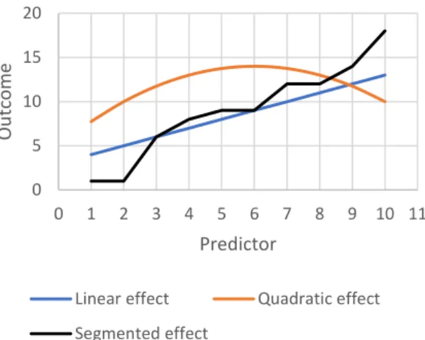
would have identical effects on another psychologi-cal attribute (e.g., job performance; Schmidt, 2002), despite the equal differences in numeric scores (100 to 120, 120 to 140). Differences in scores on a variable that does not represent varying magnitudes of a ho-mogeneous quantitative attribute but rather quali-tative differences in the properties of participants may result in such a variable having distinctly non-linear effects on other variables (see Figure 1).
Figure 1. Illustration of three types of effect. The first is a linear effect. The second is a quadratic effect—an effect that is not linear, but that can readily be specified within a linear regression framework. The third is a non-linear effect that takes the form of a segmented function, where the effect of the predictor variable itself changes abruptly as the predictor variable increases. This kind of effect is plausible when the predictor variable is ordinal, but can-not readily be accommodated within a linear regression framework (at least not without applying a piecewise model).
What can researchers do about this? Statistical analyses that permit the specification of non-linear relationships obviously do exist (e.g., Cleveland & Devlin, 1988). However, psychological theories are rarely specific enough to imply the specific func-tional form of relationships. Non-linear models can be selected based on empirical data, but basing such model specification decisions on empirical data alone may (at least in the absence of cross-valida-tion) risk overfitting—i.e., selecting overly complex nonlinear models that do not generalise well outside the sample they are trained on (Babyak, 2004; Haw-kins, 2004). In the field of statistical learning, this
problem is known as the “bias-variance trade-off” (James et al., 2013, p. 33). If we apply a simple model which incorporates inaccurate assumptions (e.g., linear relationships), the resulting estimates may be substantially biased. Applying a more flexible model (e.g., a polynomial model) may reduce this bias, but at the cost of producing estimates that are more variable across datasets (e.g., overfitting). In the ab-sence of a purely statistical solution, this problem may be addressed by the development of theory to be more specific about the functional form of rela-tionships, as occurs in mathematical psychology (see Navarro, 2020).
Where models assuming linear relationships are applied, it is important to apply diagnostic proce-dures that can detect the presence of non-linearity. Such diagnostics may allow researchers to under-stand and communicate to readers the degree to which an assumption of linearity is a reasonable
ap-proximation of reality in the specified case, and the
consequent degree to which additional uncertainty may surround the results. Although a detailed de-scription of methods for detecting non-linearity in relationships is beyond the scope of this paper, per-haps the most well-known method is plotting resid-uals against predicted (“fitted”) values to visually identify the presence of a non-linear pattern (see Gelman & Hill, 2007). More formal tests of non-line-arity in the context of regression include the RESET test (Ramsey, 1969) and the rainbow test (Utts, 1982).
Conclusion
At this point it should be clear that I see little rea-son for contemporary researchers to rigidly follow Stevens’ dictums about which statistical analyses are admissible with data of particular levels of meas-urement. A number of strong objections to Stevens’ dictums have been raised in the methodological lit-erature, of which perhaps the most fundamental is that his rules assume a goal on the part of the re-searcher to achieve a type of generalisation (infer-ences that apply across a class of coding rules) that may not be of interest to the researcher. Further-more, most statistical tests do not directly require assumptions about levels of measurement. How-0 5 10 15 20 0 1 2 3 4 5 6 7 8 9 10 11 Ou tco m e Predictor
Linear effect Quadratic effect
ever, statistical assumptions and measurement-the-oretic concerns do intersect in important ways9. My
suggestion that contemporary researchers do not need to follow Stevens’ rules exactly as he stated them should not be read as implying that research-ers can safely set aside measurement-theoretic concerns. Indeed, much as Michell (1986) suggests, measurement-theoretic issues do have implications for statistical analysis, just not the simple implica-tions proposed by Stevens. I suggest that research-ers focus on whether the statistical assumptions of the analyses they wish to perform are consistent with the observations they have collected, consider-ing in doconsider-ing so how the plausibility of these assump-tions may be affected by the level of measurement of the observations. The assumptions that are made should be clearly communicated to readers and in-terrogated for plausibility, based both on a priori considerations (e.g., is it likely that an ordinal varia-ble could have linear effects?) and empirical ones (e.g., to what extent is this set of observations con-sistent with a linear relationship?)
Author Contact
Correspondence regarding this article should be addressed to Matt Williams, School of Psychology, Massey University, Private Bag 102904, North Shore,
Auckland, New Zealand. Email:
M.N.Williams@mas-sey.ac.nz ORCID:
https://orcid.org/0000-0002-0571-215X
Conflict of Interest and Funding
I report no conflicts of interest. This study did not receive any specific funding.
Author Contributions
I am the sole contributor to the content of this article.
9 Sometimes this connection between measurement and
analysis is very direct. Consider, for example, the “Mat-thew effect” in reading, where investigating the claimed
Open Science Practices
This article earned no Open Science Badges be-cause it is theoretical and does not contain any data or data analyses. However, the R-code provided in the OSF project was fully reproducible with the given example data.
References
Altman, D. G., & Bland, J. M. (2009). Parametric v non-parametric methods for data analysis.
BMJ, 338, a3167.
https://doi.org/10.1136/bmj.a3167 Babyak, M. A. (2004). What you see may not be
what you get: A brief, nontechnical introduc-tion to overfitting in regression-type models.
Psychosomatic Medicine, 66(3), 411–421.
https://doi.org/10.1097/01.psy.0000127692.23 278.a9
Borsboom, D. (2005). Measuring the mind:
Concep-tual issues in contemporary psychometrics.
Cambridge University Press.
Bridgman, P. W. (1927). The logic of modern physics. Macmillan.
Bürkner, P.-C., & Vuorre, M. (2019). Ordinal regres-sion models in psychology: A tutorial. Advances
in Methods and Practices in Psychological Sci-ence, 2(1), 77–101.
https://doi.org/10.1177/2515245918823199 Campbell, N. R. (1920). Physics: The elements.
Cam-bridge University Press.
Carifio, J., & Perla, R. (2008). Resolving the 50-year debate around using and misusing Likert scales. Medical Education, 42(12), 1150–1152.
https://doi.org/10.1111/j.1365-2923.2008.03172.x
Chang, H. (2009). Operationalism. In E. N. Zalta (Ed.), The Stanford Encyclopedia of Philosophy.
https://plato.stanford.edu/ar-chives/fall2009/entries/operationalism/ Cheung, F., & Lucas, R. E. (2014). Assessing the
va-lidity of single-item life satisfaction measures: Results from three large samples. Quality of
phenomenon—compounding differences over time be-tween stronger and weaker readers—clearly requires the empirical comparison of differences (i.e., an interval scale; see Protopapas et al., 2016).
Life Research, 23(10), 2809–2818.
https://doi.org/10.1007/s11136-014-0726-4 Cleveland, W. S., & Devlin, S. J. (1988). Locally
weighted regression: An approach to regres-sion analysis by local fitting. Journal of the
American Statistical Association, 83(403), 596–
610.
https://doi.org/10.1080/01621459.1988.104786 39
Cliff, N. (1996). Answering ordinal questions with ordinal data using ordinal statistics.
Multivari-ate Behavioral Research, 31(3), 331–350.
https://doi.org/10.1207/s15327906mbr3103_4 Cozby, P. C., & Bates, S. C. (2015). Methods in
behav-ioral research (12th ed.). McGraw-Hill.
Dougherty, C. (2007). Introduction to Econometrics (3rd ed.). Oxford University Press.
Ferguson, A., Myers, C. S., Bartlett, R. J., Banister, H., Bartlett, F. C., Brown, W., Campbell, N. R., Craik, K. J. W., Drever, J., Guild, J., Houstoun, R. A., Irwin, J. O., Kaye, G. W. C., Philpott, S. J. F., Richardson, L. F., Shaxby, J. H., Smith, T., Thouless, R. H., & Tucker, W. S. (1940). Final re-port of the committee appointed to consider and report upon the possibility of quantitative estimates of sensory events. Report of the
Brit-ish Association for the Advancement of Science, 2, 331–349.
Gelman, A., & Hill, J. (2007). Data analysis using
re-gression and multilevel/hierarchical models.
Cambridge University Press.
Hand, D. J. (1996). Statistics and the theory of measurement. Journal of the Royal Statistical
Society: Series A (Statistics in Society), 159(3),
445–492. https://doi.org/10.2307/2983326 Hawkins, D. M. (2004). The problem of overfitting.
Journal of Chemical Information and Computer Sciences, 44(1), 1–12.
https://doi.org/10.1021/ci0342472 Heiman, G. W. (2001). Understanding research
methods and statistics: An integrated introduc-tion for psychology (2nd ed.). Houghton Mifflin.
Hesterberg, T., Moore, D. S., Monaghan, S., Clipson, A., & Epstein, R. (2002). Bootstrap methods and permutation tests. In D. S. Moore & G. P. McCabe (Eds.), Introduction to the practice of
statistics (4th ed.). Freeman.
Hölder, O. (1901). Die axiome der quantität und die
lehre vom mass. Teubner.
James, G., Witten, D., Hastie, T., & Tibshirani, R. (2013). An introduction to statistical learning (Vol. 112). Springer.
Jamieson, S. (2004). Likert scales: How to (ab) use them. Medical Education, 38(12), 1217–1218.
https://doi.org/10.1111/j.1365-2929.2004.02012.x
Judd, C. M., Smith, E. R., & Kidder, L. H. (1991).
Re-search methods in social relations (6th ed.). Holt
Rinehart and Winston.
Kaplan, R. M., & Saccuzzo, D. P. (2018). Psychological
testing: Principles, applications, and issues (9th
ed.). Cengage.
Krantz, D. H., Suppes, P., & Luce, R. D. (1971).
Foun-dations of measurement: Additive and polyno-mial representations (Vol. 1). Academic Press.
Kuzon, W., Urbanchek, M., & McCabe, S. (1996). The seven deadly sins of statistical analysis. Annals
of Plastic Surgery, 37, 265–272.
https://doi.org/10.1097/00000637-199609000-00006
Liddell, T. M., & Kruschke, J. K. (2018). Analyzing or-dinal data with metric models: What could pos-sibly go wrong? Journal of Experimental Social
Psychology, 79, 328–348.
https://doi.org/10.1016/j.jesp.2018.08.009 Luce, R. D., Suppes, P., & Krantz, D. H. (1990).
Foun-dations of Measurement: Representation, axio-matization, and invariance. Academic Press.
McBurney, D. H. (1994). Research methods (3rd ed.). Brooks/Cole.
McGrane, J. A. (2015). Stevens’ forgotten crossroads: The divergent measurement traditions in the physical and psychological sciences from the mid-twentieth century. Frontiers in Psychology,
6. https://doi.org/10.3389/fpsyg.2015.00431
Michell, J. (1986). Measurement scales and statis-tics: A clash of paradigms. Psychological
Bulle-tin, 100(3), 398–407.
https://doi.org/10.1037/0033-2909.100.3.398 Michell, J. (1999). Measurement in psychology: A
critical history of a methodological concept.
Cambridge University Press.
Michell, J. (2007). Representational theory of meas-urement. In M. Boumans (Ed.), Measurement in
Michell, J. (2012). Alfred Binet and the concept of heterogeneous orders. Frontiers in
Quantita-tive Psychology and Measurement, 3, 261.
https://doi.org/10.3389/fpsyg.2012.00261 Michell, J., & Ernst, C. (1996). The axioms of
quan-tity and the theory of measurement: Translated from part I of Otto Hölder’s German text “Die axiome der quantität und die lehre vom mass.”
Journal of Mathematical Psychology, 40(3), 235–
252. https://doi.org/10.1006/jmps.1996.0023 Navarro, D. (2020). If mathematical psychology did
not exist we would need to invent it: A case study in cumulative theoretical development
[Preprint]. PsyArXiv.
https://doi.org/10.31234/osf.io/ygbjp
Neuman, W. L. (2000). Social research methods (4th ed.). Allyn & Bacon.
Price, P. (2012). Research methods in psychology. Saylor Foundation.
Protopapas, A., Parrila, R., & Simos, P. G. (2016). In search of Matthew effects in reading. Journal of
Learning Disabilities, 49(5), 499–514.
https://doi.org/10.1177/0022219414559974 Ramsey, J. B. (1969). Tests for specification errors in
classical linear least-squares regression analy-sis. Journal of the Royal Statistical Society:
Se-ries B (Methodological), 31(2), 350–371.
https://doi.org/10.1111/j.2517-6161.1969.tb00796.x
Ray, W. J. (2000). Methods: Toward a science of
be-havior and experience (6th ed.). Wadsworth.
Schmidt, F. L. (2002). The role of general cognitive ability and job performance: Why there cannot be a debate. Human Performance, 15(1–2), 187– 210.
https://doi.org/10.1080/08959285.2002.9668 091
Sherry, D. (2011). Thermoscopes, thermometers, and the foundations of measurement. Studies
In History and Philosophy of Science Part A, 42(4), 509–524.
https://doi.org/10.1016/j.shpsa.2011.07.001 Stevens, S. S. (1946). On the theory of scales of
measurement. Science, 103(2684), 677–680. https://doi.org/10.1126/science.103.2684.677 Sullivan, T. J. (2001). Methods of social research.
Harcourt College Publishers.
Suppes, P., & Zinnes, J. L. (1962). Basic measurement
theory. Stanford University.
Tal, E. (2017). Measurement in science. In E. N. Zalta (Ed.), The Stanford Encyclopedia of Philosophy.
https://plato.stanford.edu/ar-chives/fall2017/entries/measurement-science Utts, J. M. (1982). The rainbow test for lack of fit in
regression. Communications in Statistics -
The-ory and Methods, 11(24), 2801–2815.
https://doi.org/10.1080/03610928208828423 Velleman, P. F., & Wilkinson, L. (1993). Nominal,
or-dinal, interval, and ratio typologies are mis-leading. The American Statistician, 47(1), 65–72. https://doi.org/10.2307/2684788
Wechsler, D., Coalson, D. L., & Raiford, S. E. (2008).
WAIS-IV technical and interpretive manual.
Pearson.
Westfall, J., & Yarkoni, T. (2016). Statistically con-trolling for confounding constructs is harder than you think. PLOS ONE, 11(3), e0152719. https://doi.org/10.1371/journal.pone.0152719 Williams, M. N., Grajales, C. A. G., & Kurkiewicz, D.
(2013). Assumptions of multiple regression: Correcting two misconceptions. Practical
As-sessment, Research & Evaluation, 18(11).
https://scholar-works.umass.edu/pare/vol18/iss1/11/ Zigmond, A. S., & Snaith, R. P. (1983). The hospital
anxiety and depression scale. Acta Psychiatrica
Scandinavica, 67(6), 361–370.
https://doi.org/10.1111/j.1600-0447.1983.tb09716.x
Zumbo, B. D., & Kroc, E. (2019). A measurement is a choice and Stevens’ scales of measurement do not help make it: A response to Chalmers.
Edu-cational and Psychological Measurement, 76(6),
1184–1197.