Smoke spread calculations for fires in
underground mines
Rickard Hansen
Studies in Sustainable Technology 2010:07
Mälardalen University
Summary
This report is part of the research project “Concept for fire and smoke spread prevention in mines”, conducted by a research group at Mälardalen University.
The project is aimed at improving fire safety in mines in order to obtain a safer working
environment for the people working for the mining companies in Sweden or for visitors in mines open to the public.
This report deals with the issue on smoke spread calculations for fires in underground mines. The main purposes of the report are:
- Using both one- or two-dimensional calculation models as well as three-dimensional
CFD calculation models.
- Positioning the design fires (a pool fire, a fire in a loader, a fire in a loader in a sprinklered
drift, a cable fire and a bus fire) at various sites with respect to for example the ventilation system.
- Investigating the complexities of the various models, their limitations and deficiencies etc.
- Comparing the results from the calculation models with each other and with experimental
data where applicable and available.
The work in this report started with describing smoke spread in underground mines in general and then continuing with describing three types of calculation models used in this report. After that calculations and simulations were conducted – using the three models – for the five
designated design fire scenarios and the results were presented for strategic sites with respect to egress safety and the intervention of the fire and rescue services. The results from the CFD simulations were thereafter validated with respect to flame temperature and grid size
convergence. It is misleading to fully compare the outputs of the three calculation models with each other without considering the differences and limitations of the three models as they are based upon different assumptions that differ considerably. For example the hand calculation expressions and the mine ventilation network simulation program assume unidirectional flow in the drifts compared with FDS that account for multi directional flows in the drifts. Also the hand calculation expressions and the mine ventilation network simulation program both assume complete mixture of air and fire gases while FDS does not make that assumption. Visibility is not one of the output parameters of the mine ventilation network simulation program, thus limiting the available data for comparison. But one of the purposes of this report was to investigate the complexities, limitations and deficiencies of the involved models.
The advantage of FDS is the fact that it will model the area closest to the fire most accurately of the three models, for example accounting for multi directional flows in the near area of the fire. The disadvantages of the models are for example that it is not possible to fully account for the highly variable heat release rate of for example a fire in a tyre or in a vehicle when using a mine ventilation network program, as the ramp up to the maximum heat release rate is assumed to be linear and that every fire in a branch is assumed to be constant after reaching the maximum heat release rate. This does not apply to heat release rate curves that are uniform in shape such as a pool fire; in this case the heat release rate values used will be practically the same in all three types of calculation models.
Also the time periods of the simulations differ between the three models as the simulations in FDS will become impractically long as the time to simulate increases due to higher computational requirements. Thus only the first 10-20 minutes were simulated in FDS and so the chance of comparison in for example the case of the fire in the loader is strongly limited.
When comparing the results of the three calculation models the following conclusions can be made:
- The mine ventilation network simulation program generally shows higher temperatures at
the measuring points compared with the outputs of the other two models. One probable reason for this is that the heat release rate could not be represented as adequately as for the other two models; in all cases the heat release rate levels were higher for the mine ventilation network simulation program.
- Generally the hand calculations showed much lower visibility figures than the CFD
model. One reason for this – besides the fact that we are dealing with two models with vastly different approaches - is most likely in the difference in the types of smoke characteristic factors used in the two types of models.
- The FDS simulations generally showed small changes in temperature when comparing
with the other two models. This could be attributed to the fact that the measuring points are positioned at fairly large distances from the fire and thus the fire gases will cool considerably. Also the maximum heat release rate of some of the fires was small - ~1 MW – and thus the impact on the nearby environment will be limited.
- The results of the hand calculations with respect to the visibility is a good approximation
for the design fires with fairly low maximum heat release rate as the stratification in this case will be almost nonexistent and thus the smoke spread can be assumed to be equal to the ventilation velocity in a drift (one dimensional smoke spread).
- With respect to the egress safety the visibility will be the critical factor. In the case of the
pool fire (design fire) the visibility will start to decrease at an early stage of the fire both according to the hand calculations and the FDS simulation. After approximately a few minutes the visibility in a large section of the connecting main ramp will be affected due to the open nature of the area. Thus the egress will have to take place at an early stage in order to ensure safety. Regarding the fire in the loader, the fire in the parking drift and
minutes, but the facts that the FDS simulation showed no differences in visibility and that the heat release rate is relatively small in all three cases (<1 MW) would indicate that the visibility would be affected but in a limited manner and thus the egress safety will not be largely affected during the first 10-20 minutes due to for example the large spaces in the mine drifts. With respect to the bus fire the same conclusions are drawn as in the case of the pool fire except that the FDS simulation predicts a much slower smoke spread than the results from the hand calculations.
- With respect to the intervention from the fire and rescue services the visibility will also be
the critical factor as for the egress safety. The loader fire in the sprinklered drift and the cable fire should generally not pose any large problem to the intervention of the fire and rescue service, as the maximum heat release is small and the smoke spread largely limited. But the pool fire, the loader fire and the bus fire will be problematic to the intervention of the fire and rescue service as the maximum heat release is large and the smoke spread is extensive affecting a large area before the arrival of the fire and rescue service (>30 minutes). Thus the fire and rescue service will have to start the intervention at a large distance from the site of the fire and work its way towards the fire. This will take a long time and will decrease the chance of rescuing any personnel left in the area.
As no data from conducted full-scale fire experiments were found that were applicable to any of the five design fire scenarios, future work should deal with validating the results of the three models with experimental results from conducted full scale fire tests corresponding to any of the five design fire scenarios. In this case more profound comparisons and conclusions can be drawn. The work and reflections from this report can be used when working on the full-scale fire experiment.
Measuring points should be placed in the near vicinity to the fire as well as sites further away from the fire (> 50 m), this in order to effectively investigate and compare the results of one- and two-dimensional models versus a three dimensional model.
Also further and deeper studies of the applied mine ventilation network simulation program should be performed, investigating for example the assumptions and calculation models behind the specific software.
Preface
This report is part of the research project “Concept for fire and smoke spread prevention in mines”, conducted by a research group at Mälardalen University.
The project is aimed at improving fire safety in mines in order to obtain a safer working
environment for the people working for the mining companies in Sweden or for visitors in mines open to the public.
The following organisations are participating in the project: Mälardalen University, LKAB, Sala Silvergruva, Stora Kopparberget, Brandskyddslaget and Swepro Project Management.
Contents
Summary ... 2
1. Introduction ... 7
2. Background ... 8
3. Theory: smoke spread and calculation models ... 10
3.1 One- and two-dimensional calculation models ... 10
3.1.1 Hand calculations ... 11
3.1.2 Mine ventilation network ... 12
3.2 Three-dimensional CFD models ... 13
4. Results from calculation models ... 15
4.1 Pool fire in the main ramp ... 16
4.1.1 Hand calculations ... 17
4.1.2 Mine ventilation network ... 17
4.1.3 CFD model ... 18
4.2 Vehicle fire in the production area ... 18
4.2.1 Hand calculations ... 19
4.2.2 Mine ventilation network ... 19
4.2.3 CFD model ... 20
4.3 Vehicle fire in a parking drift ... 20
4.3.1 Hand calculations ... 21
4.3.2 Mine ventilation network ... 22
4.3.3 CFD model ... 22
4.4 Cable fire at the visitor museum ... 23
4.4.1 Hand calculations ... 23
4.4.2 Mine ventilation network ... 24
4.4.3 CFD model ... 24
4.5 Bus fire at the visitor museum ... 25
4.5.1 Hand calculations ... 25
4.5.2 Mine ventilation network ... 26
4.5.3 CFD model ... 26
5. Validation of results from CFD model ... 28
5.1 Adiabatic flame temperature ... 28
5.2 Size of grid ... 28
6. Discussion and conclusions ... 29
References ... 32 Appendix 1-15
1. Introduction
Research regarding fire safety in mines has so far mainly been directed towards coal mines. Thus the need for recommendations, models, engineering tools etc for non-coal underground mines are in great need.
The aim of the current research project “Concept for fire and smoke spread prevention in mines” is to improve fire safety in mines in order to obtain a safer working environment for the people working for the mining companies in Sweden or for visitors in mines open to the public. The fire safety record in mines in Sweden is in general good with very few fire accidents that have occurred. The main reason is that there is a great awareness of the fire safety problems in mines. The awareness comes from the fact that escape routes from mines are generally limited. The reason why there is a limited amount of escape routes is that it is expensive to construct extra escape routes which are not a part of the tunnel mining system. The costs to build extra escape tunnels may be better spent on different safety equipment or systems for fire prevention or evacuation. Such systems can be ventilation systems, fire fighting equipment or rescue chambers located at different places in the mines.
The project consists of different steps, where each step is based on results and knowledge from the earlier steps. The steps are: literature survey, inventory of technical and geometrical
conditions, calculation of smoke spread, model scale tests and reports and recommendations. All results will be compared and evaluated against earlier experiences.
This report deals with the step regarding calculation of smoke spread. The main purposes of the report are:
- Using both one- or two-dimensional calculation models as well as three-dimensional
CFD calculation models.
- Positioning the design fire at various sites with respect to for example the ventilation
system.
- Investigating the complexities of the various models, their limitations and deficiencies etc.
Comparing the results from the calculation models with each other and with experimental data where applicable and available.
The output of the project will mainly consist of: performed tests, written reports and
recommendations within the mining companies regarding fire safety work, recommendations and the engineering tools for calculation of fire development and smoke spread in mines, and the mathematical models and the test results for future validation.
2. Background
The fire safety problems in mines are in many ways very similar to the problems discussed in road, rail and metro tunnels under construction. There is usually a limited amount of escape routes and the only safe havens are the safety chambers consisting of steel containers with air supply within and rescue rooms which have a separate ventilation system and will withstand a fire for at least 60 minutes.
Rescue operation is hard to perform when the attack routes often are equal with the possible path for smoke to reach the outside. The possibilities for a safe evacuation and a successful fire and rescue operation are strongly linked to the fire development and the smoke spread in these kinds of constructions.
For mining companies the problems with evacuation and rescue operations in case of fire are closely linked to policies, work environment protection and their systematic fire safety work. An accident not only can cause injuries, or in the worst case deaths, but also large costs due to production losses, reparations and loss in good-will.
The main problem with mines today is that they have become more and more complicated, with endless amount of shafts, ramps and drifts, and it is difficult to control the way the smoke and heat spread in case of a fire. The ventilation strategy is of the greatest importance in such cases in combination with the fire and rescue strategies. Since there are very few fires that occur, the experience of attacking such fires in real life is little. New knowledge about fire and smoke spread in complicated mines consisting of ramps is therefore of importance in order to make reasonable strategies for the personnel of the mining company and the fire and rescue services. The main experience from fighting mine fires comes from old coal mines, which are usually quite different in structure compared to mines in Sweden which mainly work with metalliferous rock products. In Sweden the mines consist of either active working mines with road vehicle traffic and elevator shafts for transportation of people and products or old mines allowing visitors. In some cases it is a combination of both types.
As the mine industry is changing and the challenging techniques are developed, the measures to guarantee the safety of personnel need to be adjusted. The new technology means new types of fire hazards, which in turn requires new measures to cope with the risks. New equipment means new types of fire development. The knowledge about fire developments in modern mines is relatively limited. The fire development of vehicles transporting material inside the mines is usually assumed to be from ordinary vehicles, although the vehicles may be considerably different in construction and hazard. The difference may mainly be in the amount of liquid (e.g. hydraulic oil) and the size of the rubber tyres.
The smoke spread in underground mines will dictate highly important issues such as egress safety and the likelihood of a successful intervention of the rescue services, thus the importance of this issue.
Based upon the five representative design fires for LKAB mines that were selected, developed and presented in the report Design fires in underground mines [1], calculations models were applied. The calculation models that were used were: one- and two-dimensional calculation models and three-dimensional CFD models. When applying the calculation models the position of the design fire was varied as well as external parameters influencing the smoke spread – such as ventilation rates etc. After finishing the calculations, the results from the calculation models were compared with each other and with experimental data if applicable and available.
3. Theory: smoke spread and calculation models
The behaviour of the smoke spread in a mine drift is largely determined by the smoke
stratification. The smoke stratification in its turn is highly dependent upon the air velocity in the mine drift and the position of interest with respect to the fire. Three typical air velocity ranges are identified when describing the smoke stratification:
- Low or no forced air velocity (0-1 m/s). Within this range the smoke stratification is high
in the near area of the fire.
- Moderate forced air velocity (1-3 m/s). Within this range the smoke stratification in the
near area of the fire is largely affected by the air velocity.
- High forced air velocity (>3 m/s). Within this range the smoke stratification is low
downstream from the fire. [2]
The smoke stratification will also be dependent upon the distance from the fire to the point of interest, the further away from the fire the vertical temperature gradients will decrease and thus also the smoke stratification.
Another influencing phenomenon is the so called backlayering, i.e. smoke travelling in the opposite direction with respect to the ventilation flow. Backlayering usually occurs when the air velocity is within the low or moderate range.
A fire with a high heat release rate may cause two types of effects that will influence the smoke spread as well as the ventilation:
- Throttle effect.
- Buoyancy effect.
The throttle effect is caused by the increase in volume of the air mass as it passes through the fire site. The increased volume in the mine drift immediately downstream of the fire site requires additional ventilation pressure to overcome the throttle effect and maintain the flow. The throttle effect occurs at the area closest to the fire site.
The buoyancy effect occurs in a mine drift with an inclination where the heat from the fire causes an increase in the temperature and thus a decrease in the density of the air and the smoke
downstream of the fire. This effect will work with the ventilation in rising drifts and work against the ventilation – causing reversal - in declining drifts.
When quantifying the smoke spread the calculation models are divided into two main groups based upon the number of possible dimensions: one- and two-dimensional calculation models and three-dimensional (CFD) calculation models.
3.1.1 Hand calculations
If assumed that the bulk flow of the fire gases are completely mixed – which is the case for the furthest region from the fire where insignificant stratification is taking place and the smoke layer has descended to the floor level - the average gas temperature and visibility can be calculated as a function of the distance from the fire.
The average gas temperature over the entire cross-section at the fire can be calculated using the following equation [2]: p a a x avg c m Q T T ⋅ + = = & & )( 3 2 ) ( 0 , τ τ (1) Where: a
T is the ambient temperature
)
(τ
Q& is the HRR at time τ
a
m& is the mass flow in the mine drift
p
c is the heat capacity
The transport time, τ, is calculated using the following expression:
u x t − =
τ
(2) Where:u is the air velocity in the mine drift
x is the distance between the fire and the place of interest
The average gas temperature over the entire cross-section of the drift at x m from the fire and at
time t can be calculated using the following equation and assuming that the wall temperature is
the same as the ambient temperature:
[
]
macp x P h a x avg a avg x t T T T e T ⋅ ⋅ ⋅ − = − ⋅ + = ( ) & ) , ( , 0 τ (3) Where:h is the lumped heat transfer coefficient
The average visibility over a cross-section in a mine drift (at location x ) can be calculated using the following expression [2]:
mass ec D Q H A u V ⋅ ⋅ ⋅ ⋅ = ) ( 87 . 0
τ
& (4) Where:A is the cross-sectional area of the mine drift
ec
H is the effective heat of combustion
mass
D is the mass optical density
3.1.2 Mine ventilation network
The mine ventilation system of an underground mine is often referred to as the mine ventilation network. The mine ventilation network consists of a complex system of airways, fans and other devices. The purposes of the network are to: ensure adequate supply and quality of air, and to provide a tool for smoke evacuation [3].
When solving a complex mine ventilation network, parameters such as the characteristics of the flowing air, airways, fans; the relationship of flows and head losses in series and parallel circuits etc. are combined and solved iteratively using Kirchoff’s current and voltage laws [3]. The sheer complexity of a mine ventilation network generally makes it solvable only by using applicable software. Most software programs use techniques such as the Hardy Cross iterative technique to converge to a solution, i.e. the airflow, pollutant and temperature distributions. The software can either assume compressible air or incompressible air. All mine ventilation network software assumes unidirectional flows in the mine drifts. Most software assumes immediate and complete mixing of gases, thus not accounting for the issue with stratified flow.
Some software is based upon the assumption of constant airflow rates – either the airflow rates that prevailed before the fire or those which result from an equilibrium between fire-generated thermal forces and ventilating forces. The first assumption would apply to the early stages of a fire. The second assumption means combining steady-state with real-time calculations [4]. During the work on this report the mine ventilation network software Ventgraph [5] was applied. Ventgraph is an integrated set of computer programs providing tools for solution of ventilation problems. Ventgraph uses earlier work from Polish scientists regarding the description of phenomena influencing unsteady processes of flow of air and mixtures of air and fire gases.
- Module for creation of input data: in this module input data such as the network structures, calculation of resistance values of branches and pressures in nodes etc. are specified by the user.
- Module for design of graphical representation of the mine ventilation network: diagrams can be drawn consisting of branches, nodes, symbols of fans, arrows showing the flow direction etc. [5]
- Fire module: the module consists of for example the following parts:
- Location of the fire: the user will start with pointing out the site of the fire. After that the kind of fuel burnt is selected among the following options: oil, coal, belt and wood. Thus any other type of fuel cannot be selected. The fuel calorific value and the maximum length of fire zone are entered. After that the so called fire intensity – using a scale from 0 to 10 – is entered. The assumed content of carbon monoxide and hydrogen in combustion products are entered. Finally a time
constant of the fire development is entered. Thus it is not possible to directly enter the heat release rate values of the fire in question. Instead the user will have to adjust the fire intensity value, the time constant of the fire development etc. in order to try to replicate the desired heat release rate curve. Obviously it is very difficult to get an exact copy of the heat release rate curve. A fairly large possibility of obtaining a relatively accurate curve is when working on a pool fire where the heat release rate is fairly constant over a longer time period.
- Fire parameters: this option is similar to the “Location of the fire”, but can also be used for changing the fire parameters during the simulation (transient effects). - Sensors: locating and specifying the kind of a sensor and its measuring range. Temperature, contents of carbon dioxide and carbon monoxide are some examples of parameters that can be measured with the sensors.
3.2 Three-dimensional CFD models
Computational Fluid Dynamics (CFD) models are used to simulate and predict fluid flows, heat transfer, chemical reactions etc. The number of applicable areas is vast; you will find it being used in areas such as: aerodynamics, hydrodynamics, marine engineering, meteorology, combustion and fire dynamics.
The use of CFD models have increased tremendously during the last decade, mainly due to hardware with high performance at a lower cost.
As with other tools a CFD model must be used with caution, after a simulation the user must make a judgement whether the results are probable or not. Thus a validation of the results must be conducted, comparing with the results of experimental test work. It is important to know that calculation results from CFD models can never replace results from fire experiments, but CFD can work as a powerful complement when solving fire problems [6].
A CFD model is based upon a number of governing equations representing the conservation laws of physics:
- The mass of fluid is conserved.
- The rate of change of momentum equals the sum of the forces on a fluid particle.
- The rate of change of energy is equal to the sum of the rate of heat addition to and the rate of work performed on a fluid particle.
The governing equations contain the unknown viscous stress components. Substitution of the stresses – in order to introduce a suitable model - results in the well known Navier-Stokes equations.
The issue of turbulence is solved by for example using the so called Large Eddy Simulation (LES) where LES uses a spatial filtering operation to separate the larger and smaller eddies [6].
In this report the CFD model FDS [7] (Fire Dynamics Simulator) version 5 is used. FDS solves numerically a form of the Navier-Stokes equations suitable for the low-speed, thermally driven flow connected with smoke and heat transport from fires.
Turbulence is solved by means of the Smagorinsky form of the LES. It is also possible to perform a Direct Numerical Simulation (DNS) if the underlying numerical mesh is fine enough to solve the unsteady Navier-Stokes equations. In DNS the simulations compute the mean flow and turbulent velocity fluctuations.
FDS uses a single step chemical reaction whose products are tracked via a two-parameter mixture fraction model. The mixture fraction is a conserved scalar quantity that represents the mass fraction of one or more components of the gas at a given point in the flow field.
Radiative heat transfer is in most cases solved through the radiation transport equation for a gray gas.
4. Results from calculation models
The measuring points were chosen with respect to critical sites for the egress safety and for the rescue intervention in the Kiruna mine, thus sites such as entrance from the main ramp, area at rescue chamber etc. were chosen. The purposes of the calculations and simulations was to receive data that could be used when comparing the different models with each other and to receive data that was relevant for the quantification of the egress safety and the intervention of the fire and rescue service at the five design fire scenarios. The following sites were chosen for the five design fire scenarios:
The pool fire:
- Junction to the main ramp, approximately 30 meters from the site of the fire. - Fifty meters up along the main ramp.
- Hundred meters up along the main ramp. The fire in a loader:
- At the junction to the main ramp, approximately 50 meters from the site of the fire. - At the intake and exhaust ventilation shafts, approximately 100 meters from the site of
the fire.
The fire in a loader at a sprinklered parking drift:
- At the refuge room.
- At the entrance to the train workshop. - At the junction to the main ramp (road 22).
- Fifty meters along the tracks in the train workshop. - Hundred meters along the tracks in the train workshop. - Two hundred meters along the tracks in the train workshop. The cable fire:
- Hundred meters along the drift (blocking the egress route from the mining museum). - The junction to the main ramp (road 22), approximately two hundred meters from the
site of the fire.
- Two hundred meters along the drift (blocking all egress routes at the southern end). The bus fire:
- Hundred meters along the drift (blocking the egress route from the mining museum). - The junction to the main ramp (road 22), approximately two hundred meters from the
site of the fire.
Unfortunately visibility is not one of the output parameters of the mine ventilation network simulation program, thus the visibility is not listed in these cases.
In all the cases the drift in question was assumed to be 5 m in height and 5 m in width. Thus the
cross section area of the drift is 25 m2 and the perimeter is 20 m. The temperature in the drift in
all cases was assumed to be 11ºC.
The following transport times and mass flows were calculated and used in the hand calculations of the five design fire scenarios:
Table 1. The transport times and mass flows of the five design fire scenarios.
Scenario Transport time Mass flow [kg/s]
Pool fire t-x 30
Fire in a loader t-x/0.24 7.2
Fire in a parking drift t-2·x 15
Cable fire t-x/1.5 45
Bus fire t-2·x 15
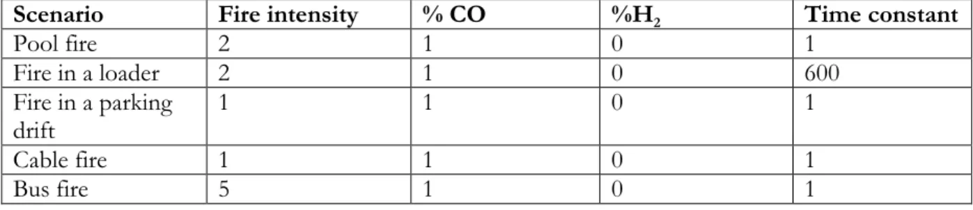
The following values for the fire intensity, carbon monoxide level, hydrogen level and time constant were used in the simulations of Ventgraph:
Table 2. The fire intensity, level of carbon monoxide and hydrogen, and the time constant of the five design fires used in Ventgraph.
Scenario Fire intensity % CO %H2 Time constant
Pool fire 2 1 0 1 Fire in a loader 2 1 0 600 Fire in a parking drift 1 1 0 1 Cable fire 1 1 0 1 Bus fire 5 1 0 1
In reality the % CO value in combustion products from the five design fires is much smaller than 1, but the smallest number accepted in the program is 1.
4.1 Pool fire in the main ramp
The place of the fire was assumed to be the diesel tank at level 1028 along road 25 (main ramp) in the Kiruna mine. During the calculations and the simulations the following heat release rate curve was used for the pool fire scenario [1]:
HRR, pool fire in main ramp 0 500 1000 1500 2000 2500 0 10 20 30 40 50 60 t (min) H R R ( k W )
Figure 1. The heat release rate curve of the pool fire in the main ramp. The ventilation velocity in the drift was assumed to be 1 m/s.
See appendix 1 for the general layout of the drift and the surroundings.
4.1.1 Hand calculations
The lumped heat transfer coefficient - h - was set to: 0.02 kW/m²·K
ec
H is set to 38.6 MJ/kg [8]
mass
D is set to 315 m2/kg [9]
The mass optical density value above is valid for fuel oil and was assumed to represent diesel fairly well.
Calculating the Tavg and V as a function of time for the three positions, see appendix 2 for the
results.
In appendix 2 a linear increase up to 315 K after 30 seconds is found for the case x=30 m.
Regarding the visibility in the same case, it drops instantaneously to almost zero after 30 seconds.
In the case of x=80 m a linear increase up to 300 K is noted after 80 seconds. The visibility
drops instantaneously to almost zero after 80 seconds.
At x=130 m a linear increase to 292 K after 130 seconds is noted. The visibility in the same
case drops instantaneously to almost zero after 130 seconds.
The resulting HRR-curve was in relative accordance with figure 1 for the first hour. Thus only the results for the first hour were used. See figure 2 for the heat release rate curve in the simulation.
Figure 2. The heat release rate curve in the simulation.
The results from the simulation showed no changes in temperature at the three measuring places.
4.1.3 CFD model
During the simulations point source measurements with respect to temperature and visibility at the three sites, average values were then calculated.
The first 10 minutes of the fire was simulated.
The outputs from the simulations are found in appendix 3.
In appendix 3 the temperature at x=30 m instantaneously increases to approximately 295 K
after approximately 1 minute. Regarding the visibility in the same case, it decreases a couple of meters starting after approximately 2 minutes.
In the case of x=80 m an instantaneous increase up to approximately 289 K is noted after
approximately 5 minutes. The visibility at the same site is not affected during the first 10 minutes.
At x=130 m an instantaneous increase up to approximately 288 K starting at approximately 4
minutes and reaching 288 K after approximately 8 minutes. The visibility in the same case is not affected during the first 10 minutes.
4.2 Vehicle fire in the production area
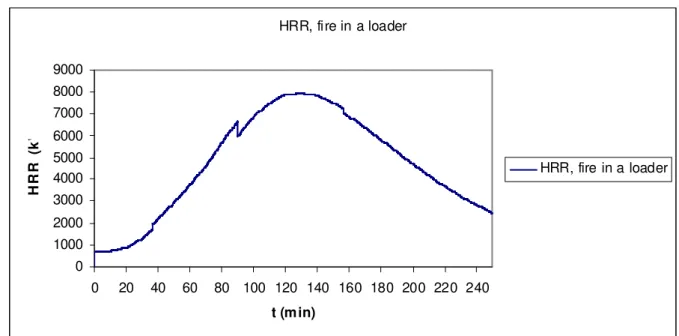
The site of the fire was chosen as the middle of the northern transversal drift at level 907 in the production area of the Kiruna mine. During the calculations and the simulations the following
HRR, fire in a loader 0 1000 2000 3000 4000 5000 6000 7000 8000 9000 0 20 40 60 80 100 120 140 160 180 200 220 240 t (m in) H R R ( k W ) HRR, fire in a loader
Figure 3. The heat release rate curve of the fire in a heavy vehicle (loader) in the production area. The ventilation velocity in the drift was assumed to be 0.24 m/s.
See appendix 4 for the general layout of the drift and the surroundings.
4.2.1 Hand calculations
The lumped heat transfer coefficient - h - was set to: 0.02 kW/m²·K
ec
H is calculated to 28 MJ/kg [1] [10]
mass
D is set to 76 m²/kg [11] using a value applicable for a truck
Calculating the Tavg and V as a function of time for the five positions, see appendix 5 for the
results.
In appendix 5 having the same shape as the heat release curve, at x=50 m the temperature
reaches its maximum value at 330 K after approximately 130 minutes. Regarding the visibility in the same case, it instantaneously drops to almost zero after approximately 5 minutes.
In the case of x=100 m the maximum value of 287 K is reached after approximately 140
minutes. The visibility at the same site drops instantaneously to almost zero after approximately 8 minutes.
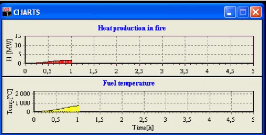
4.2.2 Mine ventilation network
The resulting HRR-curve was very difficult to get in accordance with figure 3. Thus the results of the simulations must be studied with precaution. See figure 4 for the heat release rate of the simulation.
Figure 4. The heat release rate curve of the simulation.
The results from the simulation regarding the temperature are found in appendix 6.
In appendix 6 the temperature at x=50 m increases rapidly after approximately 25 minutes and
reaching its maximum value at 623 K after approximately 40 minutes.
In the case of x=100 m the temperature starts to increase after approximately 75 minutes and
reaching its maximum value at 333 K after approximately 85 minutes.
4.2.3 CFD model
During the simulations point source measurements with respect to temperature and visibility at the two sites, average values were then calculated.
The first 20 minutes of the fire was simulated, thus only a maximum heat release rate of approximately 900 kW was accounted for.
The output from the simulations showed no detectable changes with respect to the temperature and visibility.
4.3 Vehicle fire in a parking drift
The site of the fire was chosen as the parking drift closest to the refuge room at level 1045 in the Kiruna mine. During the calculations and the simulations the following heat release rate curve was used for the vehicle fire in a parking drift scenario [1]:
Fire in a loader, in a drift protected by a sprinkler system 0 100 200 300 400 500 600 700 800 0 10 20 t (min) H R R ( k W )
Fire in a loader, in a drift protected by a sprinkler system
Figure 5. The heat release rate curve of the fire in a heavy vehicle (loader) in a parking drift protected by a sprinkler system.
The ventilation velocity in the drift was assumed to be 0.5 m/s.
See appendix 7 for the general layout of the drift and the surroundings.
4.3.1 Hand calculations
The lumped heat transfer coefficient - h - was set to: 0.02 kW/m²·K
ec
H is calculated to 28 MJ/kg [1] [10]
mass
D is set to 76 m²/kg [11] using a value applicable for a truck
Calculating the Tavg and V as a function of time for the five positions, see appendix 8 for the
results.
In appendix 8 the temperature at x=70 m instantaneously increases to 289 K after 150 seconds
and starts to decay after approximately 300 seconds. Regarding the visibility in the same case, it drops instantaneously to almost zero after 150 seconds and starts to increase after approximately 300 seconds.
In the case of x=100 m an instantaneous increase up to 286 K is noted after 210 seconds and
starts to decay after approximately 360 seconds. The visibility at the same site drops
instantaneously to almost zero after 210 seconds and starts to increase after approximately 360 seconds.
At x=150 m an instantaneous increase of one degree up to 285 K after 300 seconds and starts
to decay after approximately 420 seconds. The visibility in the same case drops instantaneously to almost zero after 300 seconds and starts to increase after approximately 420 seconds.
At x=250 m the temperature stays practically constant at 284 K. The visibility in the same case drops instantaneously to almost zero after 510 seconds and starts to increase after approximately 630 seconds.
4.3.2 Mine ventilation network
The resulting HRR-curve was very difficult to get fully in accordance with figure 5, only the first hour and a half was fairly well replicated. Thus only the results for the first hour and a half were used. See figure 6 for the heat release rate curve of the simulation.
Figure 6. The heat release rate of the simulation.
The results from the simulation regarding the temperature are found in appendix 9. In appendix 9 the temperature at the refuge room starts to increase after approximately 50 minutes and reaches a temperature of approximately 373 K after 90 minutes.
In the case of the site 50 m along the tracks the temperature starts to increase after approximately 65 minutes reaching a temperature of approximately 290 K after 90 minutes.
At the site 100 m along the tracks the temperature starts to increase after approximately 55 minutes reaching a temperature of approximately 308 K after 90 minutes.
At the site 200 m along the tracks the temperature starts to increase after approximately 70 minutes reaching a temperature of approximately 293 K after 90 minutes.
4.3.3 CFD model
During the simulations point source measurements with respect to temperature and visibility at the sites, average values were then calculated.
4.4 Cable fire at the visitor museum
The site of the fire was chosen as the drift just outside the visitor museum at level 540 in the Kiruna mine. During the calculations and the simulations the following heat release rate curve was used for the cable fire scenario [1]:
Figure 7. The HRR curve for a mixture of various types of cables on a horizontal cable tray (curve H5).
The ventilation velocity in the drift was assumed to be 1.5 m/s.
See appendix 10 for the general layout of the drift and the surroundings.
4.4.1 Hand calculations
The lumped heat transfer coefficient - h - was set to: 0.02 kW/m²·K
ec
H is set to 5.4 MJ/kg, which is applicable to PVC [10]
mass
Calculating the Tavg and V as a function of time for the five positions, see appendix 11 for the
results.
In appendix 11 the temperature at x=100 m linearly increases after approximately 3 minutes up
to 291 K and starts to decay right after that. The visibility drops instantaneously to almost zero after approximately 1 minute and starts to increase again after approximately 12 minutes.
In the case of x=200 m the temperature starts to linearly increase after approximately 4
minutes to 287 K and starts to decay right after that. The visibility at the same site drops instantaneously to almost zero after approximately 150 seconds and starts to increase after approximately 13 minutes.
4.4.2 Mine ventilation network
The resulting HRR-curve was very difficult to get fully in accordance with figure 7. Thus the results should be used with caution. See figure 8 for the heat release rate curve of the simulation.
Figure 8. The heat release rate of the simulation.
The results from the simulation regarding the temperature are found in appendix 12.
In appendix 12 the temperature 100 m along the drift starts to increase after approximately 30 minutes, reaching a maximum value of 311 K after approximately 80 minutes.
In the case of 200 m along the drift the temperature starts to increase after approximately 40 minutes, reaching a maximum value of 308 K after approximately 80 minutes.
4.4.3 CFD model
The output from the simulations showed no detectable changes with respect to the temperature and visibility.
4.5 Bus fire at the visitor museum
The site of the fire was assumed to be the same as for the cable fire. During the calculations and the simulations the following heat release rate curve was used for the bus fire scenario [1]:
HRR, Bus fire 0 1000 2000 3000 4000 5000 6000 7000 8000 9000 10000 0 10 20 30 40 50 60 70 80 90 100 110 120 130 140 150 t (min) H R R ( k W ) HRR, Bus fire
Figure 9. The heat release rate of the bus fire.
The ventilation velocity in the drift was assumed to be 0.5 m/s.
See appendix 10 for the general layout of the drift and the surroundings.
4.5.1 Hand calculations
The lumped heat transfer coefficient - h - was set to: 0.02 kW/m²·K
ec
H is calculated to 33MJ/kg [1] [10] [12], each bus seat is assumed to have a mass of 5 kg.
mass
D is set to 203 m²/kg [11]
Calculating the Tavg and V as a function of time for the five positions, see appendix 13 for the
results.
In appendix 13 the temperature – having the same shape as the heat release curve - at x=100 m
reaches its maximum value of 311 K after approximately 20 minutes. The visibility in the same case drops instantaneously to almost zero after approximately 5 minutes.
In the case of x=200 m the temperature reaches its maximum value of 286 K after
approximately 25 minutes. The visibility at the same site drops instantaneously to almost zero after approximately 8 minutes.
4.5.2 Mine ventilation network
The resulting HRR-curve was very difficult to get fully in accordance with figure 9. Thus the results should be used with caution.
Figure 10. The heat release rate curve of the simulation.
The results from the simulation regarding the temperature are found in appendix 14. In appendix 14 – having approximately the same shape as the heat release curve - the
temperature at x=100 m reaches its maximum value of approximately 483 K after
approximately 30 minutes.
In the case of x=200 m the temperature reaches its maximum value of approximately 423 K
after approximately 32 minutes.
4.5.3 CFD model
During the simulations point source measurements with respect to temperature and visibility at the three sites, average values were then calculated.
The first 23 minutes of the fire was simulated.
The output from the simulations showed no differences in temperature and visibility with respect to the measuring point at the junction to the main ramp. See appendix 15 for the results of the other two measuring points.
In the case of x=200 m the temperature starts to increase after approximately 13 minutes reaching a maximum of approximately 296 K after approximately 18 minutes and slowly
decreasing after that. The visibility at the same site decreases a few metres after approximately 18 minutes and starts to increase after that.
5. Validation of results from CFD model
Assessing the validity of the outputs of the fire model FDS is a vital part of the work.
When validating the simulations comparisons can be made to empirical solutions or data from conducted fire experiments. As no experimental data was found an empirical solution for flame temperature was evaluated when assessing the heat release rate of the design fire. The adiabatic flame temperature provides an upper limit for temperatures from the simulation model.
Furthermore the size of the grid is decisive when evaluating the accuracy of the output from the model. If the grid size is too large it will affect the accuracy negatively. Thus a grid sensitivity study was conducted.
5.1 Adiabatic flame temperature
In order to control the results of the simulations against the adiabatic flame temperature,
additional simulations were conducted where the temperature one decimetre above the surface of the fire were registered for the various fires. During these simulations the flame temperature never exceeded 1000ºC, which make the simulations realistic with aspect to the adiabatic flame temperature. If the flame temperature had exceeded 2500ºC the results of the simulations would have been limited.
5.2 Size of grid
When decreasing the size of the grid system the outputs showed fairly well consistency. Thus grid size convergence can be assumed. Decreasing the grid size further would not improve the quality of the result to any large extent but would instead be very costly with respect to computational requirements.
6. Discussion and conclusions
The work in this report started with describing smoke spread in underground mines in general and then continuing with describing three types of calculation models used in this report. After that calculations and simulations were conducted – using the three models – for the five
designated design fire scenarios and the results were presented for strategic sites with respect to egress safety and the intervention of the fire and rescue services. The results from the CFD simulations were thereafter validated with respect to flame temperature and grid size
convergence. It is misleading to fully compare the outputs of the three calculation models with each other as they are based upon different assumptions that differ considerably. For example the hand calculation expressions and the mine ventilation network simulation program assume unidirectional flow in the drifts compared with FDS that account for multi directional flows in the drifts. Also the hand calculation expressions and the mine ventilation network simulation program both assume complete mixture of air and fire gases while FDS does not make that assumption. Visibility is not one of the output parameters of the mine ventilation network simulation program, thus limiting the available data for comparison. If comparisons should be made fully it should be with corresponding full-scale experiments of the five design fire scenarios. But one of the purposes of this report was to investigate the complexities, limitations and
deficiencies of the involved models. In the text below these issues are discussed.
The advantage of the one- and two-dimensional models is the fact that the computational
requirements are considerably lower than compared with a CFD model. Also with Ventgraph it is possible to obtain fast and transient solutions even though the simulated system of mine drifts is vast and complex.
The advantage of FDS is the fact that it will model the area closest to the fire most accurately of the three models, for example accounting for multi directional flows.
The disadvantages of the models are for example that it is not possible to fully account for the highly variable heat release rate of for example a fire in a tyre or in a vehicle when using a mine ventilation network program, as the ramp up to the maximum heat release rate is assumed to be linear and that every fire in a branch is assumed to be constant after reaching the maximum heat release rate. There exists a time table function where it is possible to add additional fire branches at selected time points. But still the heat release rate in the mine ventilation network program will be very rough and approximate compared to the corresponding values used in the hand
calculations and CFD models.
This does not apply to heat release rate curves that are uniform in shape such as a pool fire; in this case the heat release rate values used will be practically the same in all three types of calculation models.
Also the time periods of the simulations differ between the three models as the simulations in FDS will become impractically long as the time to simulate increases due to higher computational requirements. Thus only the first 10-20 minutes were simulated in FDS and so the chance of comparison in for example the case of the fire in the loader is strongly limited.
When comparing the results of the three calculation models the following conclusions can be made:
- The mine ventilation network simulation program generally shows higher temperatures at the measuring points compared with the outputs of the other two models. One probable reason for this is that the heat release rate could not be represented as adequately as for the other two models; in all cases the heat release rate levels were higher for the mine ventilation network simulation program.
- Generally the hand calculations showed much lower visibility figures than the CFD model. One reason for this – besides the fact that we are dealing with two models with vastly different approaches - could be in the difference in the types of smoke
characteristic factors used in the two types of models.
- The FDS simulations generally showed small changes in temperature when comparing with the other two models. This could be attributed to the fact that the measuring points are positioned at fairly large distances from the fire and thus the fire gases will cool considerably. Also the maximum heat release rate of some of the fires was small - ~1 MW – and thus the impact on the nearby environment will be limited.
- The results of the hand calculations with respect to the visibility is a good approximation for the design fires with fairly low maximum heat release rate as the stratification in this case will be almost nonexistent and thus the smoke spread can be assumed to be equal to the ventilation velocity in a drift (one dimensional smoke spread).
- With respect to the egress safety the visibility will be the critical factor. In the case of the pool fire the visibility will start to decrease at an early stage of the fire both according to the hand calculations and the FDS simulation. After approximately a few minutes the visibility in a large section of the connecting main ramp will be affected due to the open nature of the area. Thus the egress will have to take place at an early stage in order to ensure safety. Regarding the fire in the loader, the fire in the parking drift and the cable fire the hand calculations indicate a sharp decline in visibility after a few minutes, but the facts that the FDS simulation showed no differences in visibility and that the heat release rate is relatively small in all three cases (<1 MW) would indicate that the visibility would be affected but in a limited manner and thus the egress safety will not be largely affected during the first 10-20 minutes due to for example the large spaces in the mine drifts. With respect to the bus fire the same conclusions are drawn as in the case of the pool fire except that the FDS simulation predicts a much slower smoke spread than the results from the hand calculations.
- With respect to the intervention from the fire and rescue services the visibility will also be the critical factor as for the egress safety. The loader fire in the sprinklered drift and the cable fire should generally not pose any large problem to the intervention of the fire and rescue service, as the maximum heat release is small and the smoke spread largely limited.
minutes). Thus the fire and rescue service will have to start the intervention at a large distance from the site of the fire and work its way towards the fire. This will take a long time and will decrease the chance of rescuing any personnel left in the area.
Unfortunately no data from conducted full-scale fire experiments were found that were
applicable to any of the five design fire scenarios. Thus future work should deal with validating the results of the three models with experimental results from conducted full-scale fire tests corresponding to any of the five design fire scenarios. In this case more profound comparisons and conclusions can be drawn. The work and reflections from this report can be used when working on the full-scale fire experiment.
Measuring points should be placed in the near vicinity to the fire as well as sites further away from the fire (> 50 m), this in order to effectively investigate and compare the results of one- and two-dimensional models versus a three dimensional model.
Also further and deeper studies of the applied mine ventilation network simulation program should be performed, investigating for example the assumptions and calculation models behind the software in more detail.
References
[1] Hansen R. (2010), Design fires in underground mines, report 2010:02, Mälardalen
University, Västerås
[2] Ingason, H., Fire Dynamics in Tunnels, The handbook of tunnel fire safety, Edited by Beard
A., Carvel R., Thomas Telford Ltd., London, 2005
[3] Hartman H. L., Ramani R.V., Mutmansky J.M., Wang Y.J. (1997), Mine ventilation
and air conditioning, third edition, John Wiley & Sons, Inc., Chichester
[4] Hansen R. (2010), Site inventory of operational mines – fire and smoke spread in underground
mines, report 2010:01, Mälardalen University, Västerås
[5] User’s guide, Ventgraph for Windows, Strata Mechanics Research Institute of Polish
Academy of Sciences, Cracow, 2010
[6] Versteeg H.K., Malalasekera W. (2007), An Introduction to Computational Fluid
Dynamics, second edition, Pearson Education Limited, Harlow
[7] McGrattan K. (2009), Fire Dynamics Simulator (Version 5) User’s Guide, NIST Special
Publication 1019-5, NIST, Gaithersburg
[8] Walton W.D., McElroy J., Twilley W.H., Hiltabrand R.R. (1994), Smoke
Measurements Using a Helicopter Transported Sampling Package, NIST Special Publication 995-2, NIST, Gaithersburg
[9] Personal communication with Haukur Ingason, Date: 2010-03-29
[10] The SFPE Handbook of Fire Protection Engineering, Third edition, NFPA, Quincy, 2002
[11] Steinert, C. (1994), Smoke and heat production in tunnel fires, Proceedings of the
International Conference on Fires in Tunnels, Swedish National Testing and Research Institute (SP), Borås, Sweden, 10-11 October, 1994
[12] Johansson P. and Axelsson J. (2006), Fire safety in buses – WP2 report: Fire safety review
Appendix 2. Tavg, x=30 m 265 270 275 280 285 290 295 300 305 310 315 320 0 1 2 3 4 5 6 7 8 9 10 11 12 13 14 15 16 17 18 19 20 t (min) T a v g ( K ) Tavg, x=30 m
The average gas temperature at x=30 m.
Tavg, x=80 m 275 280 285 290 295 300 305 0 1 2 3 4 5 6 7 8 9 10 11 12 13 14 15 16 17 18 19 20 t (min) T a v g ( K ) Tavg, x=80 m
Tavg, x=130 m 278 280 282 284 286 288 290 292 294 0 1 2 3 4 5 6 7 8 9 10 11 12 13 14 15 16 17 18 19 20 t (min) T a v g ( K ) Tavg, x=130 m
The average gas temperature at x=130 m.
Visibility, x=30 m 0 20 40 60 80 100 120 0 1 2 3 4 5 6 7 8 9 10 11 12 13 14 15 16 17 18 19 20 t (min) V ( m ) Visibility, x=30 m The visibility at x=30 m.
Visibility, x=80 m 0 20 40 60 80 100 120 0 1 2 3 4 5 6 7 8 9 10 11 12 13 14 15 16 17 18 19 20 t (min) V ( m ) Visibility, x=80 m The visibility at x=80 m. Visibility, x=130 m 0 20 40 60 80 100 120 0 1 2 3 4 5 6 7 8 9 10 11 12 13 14 15 16 17 18 19 20 t (min) V ( m ) Visibility, x=130 m The visibility at x=130 m.
Appendix 3. Average temperature at x=30 m 0 5 10 15 20 25 0,00 5,00 10,00 t (min) T ( C ) Average temperature at x=30 m
The average temperature at x=30 m.
Average temperature at x=80 m 0 2 4 6 8 10 12 14 16 18 0,00 5,00 10,00 t (min) T ( C ) Average temperature at x=80 m
Average temperature at x=130 m 0 2 4 6 8 10 12 14 16 18 0,00 5,00 10,00 t (min) T ( C ) Average temperature at x=130 m
The average temperature at x=130 m.
Visibility at x=30 m 27 27,5 28 28,5 29 29,5 30 30,5 0,00 5,00 10,00 t (min) V is ib il it y ( m ) Visibility at x=30 m The visibility at x=30 m.
Appendix 5. Tavg,x=50 m 260 270 280 290 300 310 320 330 340 0 20 40 60 80 100 120 140 160 180 200 220 240 t (min) T a v g ( K ) Tavg,x=50 m
The average gas temperature 50 m along the tracks. Tavg,x=100 m 282,5 283 283,5 284 284,5 285 285,5 286 286,5 287 287,5 0 20 40 60 80 100 120 140 160 180 200 220 240 t (min) T a v g ( K ) Tavg,x=100 m
Visibility, x=50 m 0 20 40 60 80 100 120 0 20 40 60 80 100 120 140 160 180 200 220 240 t (min) V ( m ) Visibility, x=50 m
The visibility at 50 m along the tracks.
Visibility, x=100 m 0 20 40 60 80 100 120 0 20 40 60 80 100 120 140 160 180 200 220 240 t (min) V ( m ) Visibility, x=100 m
Appendix 6. Temperature, x=50 m 0 50 100 150 200 250 300 0 1 0 2 0 3 0 4 0 5 0 6 0 7 0 8 0 9 0 1 0 0 1 1 0 1 2 0 1 3 0 1 4 0 1 5 0 t (min) T e m p ( C ) Temperature, x=50 m The temperature at x=50 m. Temperature, x=100 m 0 10 20 30 40 50 60 70 0 1 0 2 0 3 0 4 0 5 0 6 0 7 0 8 0 9 0 1 0 0 1 1 0 1 2 0 1 3 0 1 4 0 1 5 0 t (min) T e m p ( C ) Temperature, x=100 m The temperature at x=100 m.
Appendix 8. Tavg, x=70 m 281 282 283 284 285 286 287 288 289 290 0 1 2 3 4 5 6 7 8 9 10 11 12 13 14 15 16 17 18 19 20 t (min) T a v g ( K ) Tavg, x=70 m
The average gas temperature at x=70 m.
Tavg, x=100 m 282,5 283 283,5 284 284,5 285 285,5 286 286,5 0 1 2 3 4 5 6 7 8 9 10 11 12 13 14 15 16 17 18 19 20 t (min) T a v g ( K ) Tavg, x=100 m
Tavg, x=150 m 283,7 283,8 283,9 284 284,1 284,2 284,3 284,4 284,5 284,6 284,7 0 1 2 3 4 5 6 7 8 9 10 11 12 13 14 15 16 17 18 19 20 t (min) T a v g ( K ) Tavg, x=150 m
The average gas temperature at x=150 m.
Tavg, x=250 m 283,98 283,99 284 284,01 284,02 284,03 284,04 284,05 0 1 2 3 4 5 6 7 8 9 10 11 12 13 14 15 16 17 18 19 20 t (min) T a v g ( K ) Tavg, x=250 m
Visibility, x=70 m 0 20 40 60 80 100 120 0 1 2 3 4 5 6 7 8 9 10 11 12 13 14 15 16 17 18 19 20 t (min) V ( m ) Visibility, x=70 m The visibility at x=70 m. Visibility, x=100 m 0 20 40 60 80 100 120 0 1 2 3 4 5 6 7 8 9 10 11 12 13 14 15 16 17 18 19 20 t (min) V ( m ) Visibility, x=100 m The visibility at x=100 m.
Visibility, x=150 m 0 20 40 60 80 100 120 0 1 2 3 4 5 6 7 8 9 10 11 12 13 14 15 16 17 18 19 20 t (min) V ( m ) Visibility, x=150 m The visibility at x=150 m. Visibility, x=250 m 0 20 40 60 80 100 120 0 1 2 3 4 5 6 7 8 9 10 11 12 13 14 15 16 17 18 19 20 t (min) V ( m ) Visibility, x=250 m The visibility at x=250 m.
Appendix 9.
Temperature at the refuge room
0 20 40 60 80 100 120 0 10 20 30 40 50 60 70 80 90 t (min) T ( C )
Temperature at the refuge room
The temperature at the refuge room.
Temperature 50 m along the tracks
0 2 4 6 8 10 12 14 16 18 20 0 10 20 30 40 50 60 70 80 90 t (min) T ( C )
Temperature 50 m along the tracks
Temperature 100 m along the tracks 0 5 10 15 20 25 30 35 40 0 10 20 30 40 50 60 70 80 90 t (min) T ( C )
Temperature 100 m along the tracks
The temperature 100 m along the tracks.
Temperature 200 m along the tracks
0 5 10 15 20 25 0 10 20 30 40 50 60 70 80 90 t (min) T ( C )
Temperature 200 m along the tracks
Appendix 11. Tavg, x=100 m 280 282 284 286 288 290 292 0 1 2 3 4 5 6 7 8 9 10 11 12 13 14 t (min) T a v g ( K ) Tavg, x=100 m
The average gas temperature at x=100 m.
Tavg, x=200 m 282,5 283 283,5 284 284,5 285 285,5 286 286,5 287 287,5 0 1 2 3 4 5 6 7 8 9 10 11 12 13 14 t (min) T a v g ( K ) Tavg, x=200 m
Visibility, x=100 m 0 20 40 60 80 100 120 0 1 2 3 4 5 6 7 8 9 10 11 12 13 14 t (min) V ( m ) Visibility, x=100 m The visibility at x=100 m. Visibility, x=200 m 0 20 40 60 80 100 120 0 1 2 3 4 5 6 7 8 9 10 11 12 13 14 t (min) V ( m ) Visibility, x=200 m The visibility at x=200 m.
Appendix 12.
Temperature, 100 m along the drift
0 5 10 15 20 25 30 35 40 0 10 20 30 40 50 60 70 80 90 100 110 120 130 140150 t (min) T ( C ) Temperature, 100 m along the drift
The temperature 100 m along the drift.
Temperature, 200 m along the drift
0 5 10 15 20 25 30 35 40 0 10 20 30 40 50 60 70 80 90 100 110 120 130 140150 t (min) T ( C ) Temperature, 200 m along the drift
Appendix 13. Tavg, x=100 m 270 275 280 285 290 295 300 305 310 315 0 20 40 60 80 100 120 140 160 180 200 220 240 t (min) T a v g ( K ) Tavg, x=100 m
The average gas temperature at x=100 m.
Tavg, x=200 m 283 283,5 284 284,5 285 285,5 286 286,5 0 20 40 60 80 100 120 140 160 180 200 220 240 t (min) T a v g ( K ) Tavg, x=200 m
Visibility, x=100 m 0 20 40 60 80 100 120 0 20 40 60 80 100 120 140 160 180 200 220 240 t (min) V ( m ) Visibility, x=100 m The visibility at x=100 m. Visibility, x=200 m 0 20 40 60 80 100 120 0 20 40 60 80 100 120 140 160 180 200 220 240 t (min) V ( m ) Visibility, x=200 m The visibility at x=200 m.
Appendix 14.
Temperature, 100 m along the drift
0 50 100 150 200 250 0 10 20 30 40 50 60 70 80 90 100 110 120 130140150 t (min) T ( C ) Temperature, 100 m along the drift
The temperature 100 m along the drift.
Temperature, 200 m along the drift
0 20 40 60 80 100 120 140 160 0 10 20 30 40 50 60 70 80 90 100 110 120 130140150 t (min) T ( C ) Temperature, 200 m along the drift
Appendix 15. Temperature, 100 m 0 5 10 15 20 25 30
0,00E+00 7,00E+00 1,40E+01 2,10E+01
t (min) T ( C ) Temperature, 100 m
The average temperature 100 m along the drift.
Temperature, 200 m 0 2 4 6 8 10 12 14 16 18 20
0,00E+00 7,00E+00 1,40E+01 2,10E+01
t (min) T ( C ) Temperature, 200 m
Visibility, 100 m 24 25 26 27 28 29 30 31
0,00E+00 7,00E+00 1,40E+01 2,10E+01
t (min) V is ib il it y ( m ) Visibility, 100 m
The visibility 100 m along the drift.
Visibility, 200 m 26,5 27 27,5 28 28,5 29 29,5 30 30,5
0,00E+00 7,00E+00 1,40E+01 2,10E+01
t (min) V is ib il it y ( m ) Visibility, 200 m
The visibility 200 m along the drift.