Low Complexity Algorithm for Efficient Relay
Assignment in Unicast/Broadcast Wireless Networks
Le-Nam Hoang
∗, Elisabeth Uhlemann
∗†and Magnus Jonsson
∗∗ CERES, Halmstad University, Halmstad, Sweden † Malardalen University, V¨aster˚as, Sweden
Email:{le-nam.hoang, elisabeth.uhlemann, magnus.jonsson}@hh.se, elisabeth.uhlemann@mdh.se
Abstract—Using relayers in wireless networks enables higher
throughput, increased reliability or reduced delay. However, when building networks using commercially available hardware, concurrent transmissions by multiple relayers are generally not possible. Instead one specific relayer needs to be assigned for each transmission instant. If the decision regarding which relayer to assign, i.e., which relayer that has the best opportunity to successfully deliver the packet, can be taken online, just before the transmission is to take place, much can be gained. This is particularly the case in mobile networks, as a frequently changing network topology considerably affects the choice of a suitable relayer. To this end, this paper addresses the problem of online relay assignment by developing a low-complexity algorithm highly likely to find the optimal combination of relaying nodes that minimizes the resulting error probability at the targeted receiver(s) using a mix of simulated annealing and ant colony algorithms, such that relay assignments can be made online also in large networks. The algorithm differs from existing works in that it considers both unicast as well as broadcast and assumes that all nodes can overhear each other, as opposed to separating source nodes, relay nodes and destination nodes into three disjoint sets, which is generally not the case in most wireless networks.
Index Terms—Relay Networks, Error Probability, Latency,
Simulated Annealing, Ant Colony Optimization.
I. INTRODUCTION
Cooperative diversity in the form of relay nodes in wireless networks can be used to enable higher throughput, increased reliability, longer range or reduced delay, depending on ap-plications needs [1]–[3]. In many modern systems, signals from multiple relay nodes are available for each packet, through multiple antennas or concurrently transmitting nodes. The problem of appropriate relay selection then emerges. The cooperative protocol proposed in [4] reveals that by opportunistically selecting relayers, all nodes in the network can improve their stable throughput. However, when building networks using commercially available hardware, concurrent transmissions by multiple relay nodes is generally not possible. Instead one specific relay node needs to be assigned before each transmission instant. The problem then changes from relay selection into relay assignment, i.e., determining which relay node that has the best opportunity to successfully deliver This work is funded by the Knowledge Foundation (KKS) through the ACDC and READY projects and by the ELLIIT network. The research leading to these results has also partly been performed in the SafeCOP-project, that received funding from the ECSEL Joint Undertaking under grant agreements n𝑜692529, and from National funding.
the packet at a particular time-instance – and this decision needs to be made before the transmission actually takes place. Existing research on the relay assignment problem has mainly considered achievable data rate as the sole perfor-mance measure [5]–[9] and very few publications consider relaying for delay-sensitive applications. Deadline dependent communications are of particular interest for many emerging distributed control applications found in areas such as indus-trial automation, robotics or intelligent transport systems. In [10], however, a time-slotted scheduling problem is introduced, in which relay nodes overhear each other and are assigned to minimize the average number of packets missing their deadlines. However, the main focus of existing works has been on unicast traffic, not on broadcast. In [9], the problem of many to one is addressed and the authors consider a relay assignment policy that can be shared by many sender-receiver pairs. However, broadcast is not considered. More importantly, most existing works on relay assignment policies aim to separate source nodes, relay nodes and destination nodes into three disjoint sets, which is not necessarily the case in ad hoc networks. In [11], [12] we have addressed the problem of relay assignment for both unicast and broadcast by deriving a message dissemination scheme which minimizes the probability of error at the intended receiver(s) before a given deadline. Note that we assume that all nodes can overhear each other, i.e. the requirement on disjoint sets is no longer needed. The assumption that all nodes may overhear each other with a certain probability implies that Shannon’s channel capacity is not directly applicable and also that the algorithm is quite complex for large networks.
In mobile networks, where the frequently changing network topology considerably affects the choice of suitable relay nodes, much can be gained if the relay assignment can be made online, just before the transmission is to take place. To this end, this paper addresses the problem of online relay assignment by developing a low complexity algorithm highly able to select the set of relay nodes that is best suited to forward the message such that the reliability is maximized at the intended receiver(s) before the deadline. This paper thereby complements the proposed scheme introduced in [12]. We assume that each message is allocated a set of time-slots determined by the message delivery deadline. The aim is to maximize the reliability of delay-constrained messages given its set of available time-slots. The main contribution
1 2 3 4 5 N-1 N
...
p 1,2 p 1,3 p 1,5 p 1,4 p 1,N p 1,N-1 p 2,3 p 3,4 p 2,4 p 3,N-1 p 3,N p 3,5 p 4,N-1 p 4,N p 4,5 p 2,5 p 5,N-1 p 5,N p 2,N p N-1,N p 2,N-1Fig. 1. An intermittent fully connected network consisting of𝑁 nodes.
of this paper is a low-complexity algorithm very likely to find the optimal combination of relaying nodes such that they can be assigned to appropriate time-slots online. The search algorithm inherits the idea of ant-colony optimization and simulated annealing, and can efficiently find the optimal or close to optimal solution with a reduced computational cost compared to [12]. The numerical results demonstrate that the solutions derived from our proposed algorithm match the results of exhaustive search, which can be used as a benchmark only when the number of time-slots is small. Thereby it is possible to assign a close to optimal set of relay nodes that maximizes the reliability at the targeted receiver(s) before a given deadline, and this relay assignment can be made online also in large networks.
II. SYSTEMMODEL
In this work, we consider an intermittent fully connected network consisting of𝑁 nodes as shown in Fig. 1, where the nodes can communicate with each other through the direct links or with the help of intermediate relay nodes. The channel coefficient𝑔𝑖𝑗 between any pair of nodes(𝑖, 𝑗) is independent but not identical distributed (i.n.i.d.), characterized by its probability density function𝑓𝑔𝑖𝑗(𝑔𝑖𝑗). Every node transmits a power of 𝑃𝑡, while the noise power level is𝑁0 at each node. Define 𝜃𝑡ℎ as the correct decoding threshold, the probability that a message sent directly from node𝑖 cannot be successfully decoded at node 𝑗 is derived as [13]:
𝑝𝑖𝑗 = Pr [ 𝑃𝑡∣𝑔𝑖𝑗∣2 𝑁0 ≤ 𝜃𝑡ℎ ] = 𝜃𝑡ℎ ∫ 0 𝑓𝑔𝑖𝑗 (√ 𝛾𝑖𝑗𝑁0 𝑃𝑡 ) 2√𝛾𝑖𝑗𝑃𝑡 𝑁0 𝑑𝛾𝑖𝑗. (1)
Note that𝑝𝑖𝑗≈ 1 when there is no direct link between node 𝑖
and node 𝑗. Although the channel coefficient and the additive noise processes are assumed to be stationary for the whole time-slot, they may vary from time-slot to time-slot.
The time division multiple access (TDMA) approach is employed to avoid mutual interference, i.e., time is slotted and one time-slot is adequate to convey one packet. Each node is assumed to be equipped with a single antenna, and
1 2 3 4 5 7 6 Node 1 transmits in time-slot 1
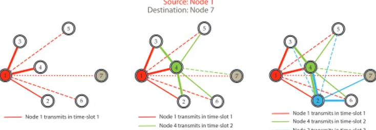
Source: Node 1 Destination: Node 7 1 2 3 4 5 7 6 Node 1 transmits in time-slot 1 Node 4 transmits in time-slot 2
1 2 3 4 5 7 6 Node 1 transmits in time-slot 1 Node 4 transmits in time-slot 2 Node 2 transmits in time-slot 3
Fig. 2. A demonstration of the proposed relaying scheme.
operate in half-duplex mode, thus it is only able to either transmit or receive one packet at a time. Suppose that a source node𝛼 wants to send to a destination node 𝛽 a single packet.𝐾𝛼𝛽time-slots are allocated for this packet, i.e.,𝐾𝛼𝛽
denotes the number of times the packet is transmitted/possibly retransmitted in the network. The value of 𝐾𝛼𝛽 depends on the application requirements on delay and reliability for that particular type of message.
Before transmitting its packet, the source node 𝛼 uses our proposed relay assignment algorithm to find the possible optimal combination of relay nodes. We denote 𝑎[𝑘], 𝑘 = 1, . . . , 𝐾𝛼𝛽 as the indexes of time-slots which are allocated to transmit this packet. In time-slot𝑎[𝑘] the relay node 𝑅[𝑘] is assigned to transmit. If 𝑅[𝑘] cannot decode the packet successfully, it will keep silent. Otherwise, it transmits the successfully decoded packet. The proposed relaying scheme can be demonstrated by an example as shown in Fig. 2. Here 𝐾17 = 3 and the sequence of relayers is {1, 4, 2}. Using
the same relaying sequence, a traditional multihop scheme would ignore the transmissions between node 1 and node 2, between node 1 and node 7, and between node 4 and node 7. Similarly, a conventional relay assignment scheme would ignore the transmissions between node4 and node 2. In contrast, our relaying scheme takes into account all possible transmissions between all nodes and fully exploit the broadcast nature of wireless communications to attain higher reliability. Note that for higher reliability, the relay nodes can be reused. For instance, in the example in Fig. 2, if𝐾17> 3, node 1, 4
and2 can be reused.
We denote the event that takes place after 𝑘 transmission attempts as 𝑒𝑘, where
𝑒𝑘=
⎧ ⎨ ⎩
1 if the relay node 𝑅[𝑘] assigned for time-slot 𝑎[𝑘] successfully decodes the packet 0 otherwise.
Moreover, denotee𝑢:𝑣 as the sequence of events that take place in time-slots 𝑎[𝑘], 𝑢 < 𝑘 < 𝑣; 𝐿𝑘 as the immediate previous time-slot prior to𝑎[𝑘] where 𝑅[𝑘] is used to relay the packet, 𝐿𝑘 = −1 if 𝑎[𝑘] is the first time that 𝑅[𝑘] is used. As shown
in [12], the probability that the event 𝑒𝑘 takes place, given that all previous events are known, can be represented by a
simplified expression as follows: Pr[𝑒𝑘 e0:𝑘−1]= 𝑘−1∏ 𝑙=𝐿𝑘+1 ( 𝑝𝑅[𝑙]𝑅[𝑘])𝑒𝑙(1−𝑒𝐿𝑘) + I {𝑒𝑘 = 𝑒𝐿𝑘} − 1 , (2) where I{𝑒𝑘 = 𝑒𝐿𝑘} is the indicator function for the event 𝑒𝑘= 𝑒𝐿𝑘, i.e.,
I{𝑒𝑘 = 𝑒𝐿𝑘} = {
1 if 𝑒𝑘= 𝑒𝐿𝑘 0 if 𝑒𝑘∕= 𝑒𝐿𝑘.
Therefore, the event 𝑒𝐾𝛼𝛽 = 0, i.e., the destination cannot receive a correct copy of the packet after 𝐾𝛼𝛽 transmission attempts, has the probability
Pr[𝑒𝐾𝛼𝛽 = 0 ] = ∑ ∀e1:𝐾𝛼𝛽−1 ∈{0,1}𝐾𝛼𝛽−1 𝐾𝛼𝛽∏−1 ℎ=𝐿𝛽+1 ( 𝑝𝑅[ℎ]𝛽 )𝑒ℎ(1−𝑒𝐿𝛽)+ I {𝑒 𝐿ℎ = 0} − 1 𝐾𝛼𝛽∏−1 𝑘=1 𝑘−1∏ 𝑙=𝐿𝑘+1 ( 𝑝𝑅[𝑙]𝑅[𝑘] )𝑒𝑙(1−𝑒𝐿𝑘)+ I {𝑒 𝑘 = 𝑒𝐿𝑘} − 1 . (3) Eq. (3) can be used to determine the optimal schedule of re-layers, both for unicast and broadcast, either using exhaustive search or in conjunction with a relevant searching algorithm. For unicast scenarios, we aim to minimize the resulting error probability at the destination node 𝛽 given 𝐾𝛼𝛽 transmission attempts. For broadcasting, we maximize the probability 𝑃𝐵 that all nodes successfully receive the broadcast message, noting that: 𝑃𝐵= Pr[𝑒𝐾𝛼𝛽 = 1, ∀𝛽 ∈ {1, 2, . . . , 𝑁} ∖ 𝛼 ] = 𝑁 ∏ 𝛽=1 𝛽∕=𝛼 (1 − Pr[𝑒𝐾𝛼𝛽= 0 ] ). (4) III. PROPOSEDSTRATEGY
In this section, we describe a low-complexity algorithm which is highly likely to find the optimal combination of relaying nodes, in order to minimize the overall probability of error at the receiver(s). The proposed algorithm is a mix of simulated annealing and ant colony algorithms, as shown in the pseudocode in Algorithm 1. The searching procedure is performed by𝑃𝑎 parallel agents and divided into two phases: exploration and exploitation. The Cost function is calculated by using the succinct eqs. (3) and (4).
In the first phase or the exploring phase, 𝑢 < 𝐸𝑥, it is set up as 0 ≪ 𝑒−𝜈 log10(Cost(𝑇 [𝑝])/Cost(𝑆[𝑝])) < 1 so that new moves are widely accepted. The new state 𝑇 [𝑝] will replace old state 𝑆[𝑝] if Cost(𝑇 [𝑝]) ≤ Cost(𝑆[𝑝]), otherwise,𝑇 [𝑝] will be accepted with the probability of accep-tance𝑒−𝜈 log10(Cost(𝑇 [𝑝])/Cost(𝑆[𝑝])). DataBest, the collection of lists of current best combinations, is updated in everyΨ+1
Algorithm 1: Find the Best Combination of Relayers
Initialize𝜈inf, 𝜈sup, 𝜎, Ψ, 𝑃𝑎, 𝐷𝑟, 𝐸𝑥;
⃗Δ ← [ ], DataBest ← [ ]; 𝑆 ← some initial candidate; 𝐵𝑒𝑠𝑡 ← 𝑃𝑎 replicas of𝑆; for𝑢 = 1 to 𝜎: 𝜈 = 𝜈inf ( 𝜈sup 𝜈inf )𝑢−1 𝜎−1 ; for𝑝 = 1 to 𝑃𝑎: for𝑣 = 0 to Ψ: 𝐶 = (𝑢 − 1)Ψ + 𝑣; if 𝑢 ≥ 𝐸𝑥: ⃗Δ[𝑝] = Tabulate (DataBest[𝑝]); 𝑇 [𝑝] = NewExploit(⃗Δ[𝑝], 𝑆[𝑝], 𝑣); if𝑢 (mod 𝐷𝑟) = 0:
Delete old records in DataBest;
else
𝑇 [𝑝] = NewExplore (𝑁, 𝜎Ψ, 𝐶, 𝑆[𝑝]);
if Cost(𝑇 [𝑝]) ≤ Cost(𝑆[𝑝]):
𝑆[𝑝] ← 𝑇 [𝑝];
else
𝑟𝑎 ← random number uniformly in (0, 1];
if𝑟𝑎≤ 𝑒−𝜈 log10(Cost(𝑇 [𝑝])/Cost(𝑆[𝑝])): 𝑆[𝑝] ← 𝑇 [𝑝];
if Cost(𝑇 [𝑝]) < Cost(𝐵𝑒𝑠𝑡[𝑝]):
𝐵𝑒𝑠𝑡[𝑝] ← 𝑇 [𝑝];
MixBest[𝑝] ← mix up 𝐵𝑒𝑠𝑡[𝑝] with random previous 𝐵𝑒𝑠𝑡[𝑝′], 𝑝′∕= 𝑝;
DataBest[𝑝] = DataBest[𝑝] ∪ MixBest[𝑝];
Function NewExplore(𝑁, Total, Counter, 𝑆):
Unit= (𝑁 − 1)length(S)/Total; Create Rand such that
∣Rand − 𝑆∣ ≤ (Total − Counter)Unit;
return Rand
Function NewExploit(⃗Δ, 𝑆, 𝑣):
if 𝑣 = 0:
Create Rand with the frequency of appearance defined by ⃗Δ;
else
Randomly choose one neighbor Rand around𝑆;
return Rand
moves. Each of the 𝑃𝑎 agents starts searching at the same initial random candidate and tries to explore widely around its own search space. The width of a new move,∣Rand − 𝑆∣, gradually narrows down over time, with the rate depending on𝜈inf, 𝜈sup, 𝜎, Ψ as explained in [14]. The end results of this
phase are𝑃𝑎separate lists DataBest[𝑝], each of which records a different path originating from the initial candidate.
On the other hand, the second phase or the exploiting phase focuses only on the vicinity of solutions listed in DataBest. For every agent 𝑝, after using Tabulate to determine the frequency of appearance of each element in𝐵𝑒𝑠𝑡[𝑝] stored in
DataBest[𝑝], we generate a newly derived candidate. In the next Ψ moves, new candidates are neighbors surrounding the derived candidate, and the best one in the bunch ofΨ+1 moves is assigned to 𝐵𝑒𝑠𝑡[𝑝]. Before recording to DataBest[𝑝], we mix up 𝐵𝑒𝑠𝑡[𝑝] with random previous 𝐵𝑒𝑠𝑡[𝑝′], 𝑝′ ∕= 𝑝. This is to combine the good features of all current finding paths, but𝐵𝑒𝑠𝑡[𝑝] is dominant. In this phase, DataBest also erases old records with the rate of𝐷𝑟, thus the procedure converges faster and reduces the risk of searching around local optimums for too long. 𝐷𝑟→ ∞ when 𝑢 is small and slowly decreases when the searching converges to the optimal solution.
One key issue in designing the heuristic algorithm is how to select appropriate neighbors Rand in the exploiting phase. Due to the structure of the network of relayers, at the beginning of the phase, we choose two or three random elements and replace them by their respective contiguous nodes. Later, we randomly choose between the following strategies: (i) choose a random element and replace by one of its contiguous nodes, (ii) swap two random adjacent elements. When the number of given time-slots increases, we can define a Tabu List to restrict the randomness in the chosen elements.
Note that the proposed algorithm does not depend on the topology of the network but on the channel characteristics related to the Cost function, thus it is applicable for a wide range of wireless settings. It consists of a triple nested for-loop, in which𝜎, Ψ and 𝑃𝑎 are independent parameters. As a result, the statements in the innermost loop are executed𝜎Ψ𝑃𝑎times. Through the numerical examples below, the algorithm is able to find the optimal solution with the number of inner moves Ψ = 2 and the number of agents 𝑃𝑎 = 10, whereas the number
of outer moves 𝜎 can be as large as 1000. In comparison, the complexity of exhaustive search is 𝒪(𝑁𝐾−1) and is thus too complex for a large number of nodes𝑁, or a large number of time-slots,𝐾.
IV. NUMERICALEXAMPLES
In this section, we exemplify by several numerical examples to illustrate the performance of the proposed strategy. We use the parameter settings suggested by the empirical results in [15], i.e. 𝑃𝑡 = 1 mW, 𝑁0 = −99 dBm, and 𝜃𝑡ℎ = 11 dB for QPSK modultion and code rate 3/4, while the pathloss exponent is 3. For any pair of nodes (𝑖, 𝑗), we assume a channel with Nakagami-𝑚 fading, together with additive white Gaussian noise (AWGN). The channel coefficient 𝑔𝑖𝑗
is characterized by an i.n.i.d Nakagami-𝑚 distribution, which has the probability density function
𝑓𝑔𝑖𝑗(𝑔𝑖𝑗) = 2𝑚𝑚𝑖𝑗 𝑖𝑗 𝑔2𝑚𝑖𝑗 𝑖𝑗−1 𝜔𝑚𝑖𝑗 𝑖𝑗 Γ(𝑚𝑖𝑗) exp ( −𝑚𝜔𝑖𝑗𝑔𝑖𝑗2 𝑖𝑗 ) , (5)
where 𝜔𝑖𝑗 = 𝐸{𝑔2𝑖𝑗} and Γ(𝑚𝑖𝑗) is the Gamma function.
Note that this distribution can also represent a wide range of multipath fading channels, e.g., the Rayleigh distribution by setting 𝑚𝑖𝑗 = 1. The Nakagami-𝑚 distribution fits well with land-mobile and indoor-mobile multipath propagation, as well as ionospheric radio links [13].
1 d 2 d 3 d 4
...
N-1 d NFig. 3. Illustration of a regular line network in which the distance between two adjacent nodes is𝑑.
Fig. 4. Performance of the transmissions between two ends of a regular line network of11 nodes, comparing ES and SA strategies.
In Fig. 4, we investigate various situations in a regular line network of 11 nodes, by varying parameter 𝑚𝑖𝑗 in the Nakagami-𝑚 distribution and the distance 𝑑 (in meters) be-tween two adjacent nodes, as illustrated in Fig. 3. Messages are originating from node1 and target node 11, their destination node. Using the exhaustive search (ES) strategy for 𝑁 − 1 relayers given𝐾 time-slots, (𝑁 −1)𝐾−1calculations of eq. (3) are needed, and thus we can only apply ES for𝐾 ≤ 7 when 𝑁 = 11. Note that when 𝐾 and 𝑁 are small, the complexity of ES is not necessarily worse than the searching heuristic. On the other hand, to verify our suggested algorithm (SA) and its search space, we execute it ten times in a row. The results from these ten consecutive implementations are all the same. For the sake of simplicity, several parameters can therefore be fixed:𝜈inf= 10−2, 𝜈sup= 10, Ψ = 2, 𝑃𝑎= 10, whereas 𝜎, 𝐷𝑟
and𝐸𝑥vary from situation to situation. As shown in Fig. 4, all results from the proposed algorithm match with the respective ones from ES. Although the structure of the regular line net-work remains the same, different 𝑑 and 𝑚𝑖𝑗 require different sequences of optimal relayers. For example, given seven time-slots, the optimal sequences of relayers are{1, 1, 3, 6, 8, 9, 10} for 𝑚𝑖𝑗 = 2, 𝑑 = 100m; {1, 1, 3, 7, 8, 9, 10} for 𝑚𝑖𝑗 = 0.5, 𝑑 = 100m; and {1, 1, 3, 7, 9, 10, 10} for 𝑚𝑖𝑗 = 0.5, 𝑑 =
50m. It is also noteworthy that the direct link between node 1 and node 11 when 𝑚𝑖𝑗 = 2, 𝑑 = 100m is worse than
when 𝑚𝑖𝑗 = 0.5, 𝑑 = 50m; however, when increasing the
amount of relaying time-slots, the reliability of a scenario in which 𝑚𝑖𝑗 = 2, 𝑑 = 100m improves faster than when 𝑚𝑖𝑗 = 0.5, 𝑑 = 50m.
d r
...
...
...
...
...
2,0 2,1 2,2 2,9 2,10 1,0 1,1 1,2 1,9 1,10 0,0 0,1 0,2 0,9 0,10 -1,0 -1,1 -1,2 -1,9 -1,10 -2,0 -2,1 -2,2 -2,9 -2,10 r r r d d d d d d d d d d d d d d r r r r r r r r r r r r r r r rFig. 5. Demonstration of a grid network of55 nodes.
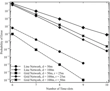
Next, we consider a grid network of55 nodes with 11 nodes in each row and𝑚𝑖𝑗 = 0.5, ∀𝑖, 𝑗, as shown in Fig. 5. For this case, exhaustive search is not tractable. The distances (in me-ters) from one node to its contiguous nodes are𝑑 horizontally and𝑟 vertically. In the unicast scenario, to compare with the respective line network of11 nodes, node (0, 0) is chosen to be the source node and the destination node is node(0, 10). The grid network performs better due to its larger space diversity. Moreover, one property of the optimal strategy is that the node closest to the destination node should be used in the last time-slot. For example, given9 time-slots, the resulting sequences of relayers are{(0,0), (0,0), (0,0), (0,5), (1,9), (0,9), 1,9), (-1,10), (1,10)} for 𝑑 = 50m, 𝑟 = 25m; {(0,0), (0,0), (0,1), (0,3), (0,4), (0,6), (0,9), (-1,10), (1,10)} for 𝑑 = 100m, 𝑟 = 25m; and{(0,0), (0,0), (0,1), (0,3), (0,4), (0,8), (0,9), (-1,10), (1,10)} for𝑑 = 100m, 𝑟 = 50m. This can be explained by rearranging (3) given 𝐾 time-slots as follows
Pr [𝑒𝐾 = 0] = ∑ ∀e𝐾−2 1 ∈{0,1}𝐾−2 𝑝𝑅0𝛽 𝐾−2∏ 𝑘=1 ( 𝑝𝑅𝑘𝛽)𝑒𝑘 𝑘−1∏ 𝑗=𝐿𝑘+1 ( 𝑝𝑅𝑗𝑅𝑘)𝑒𝑗(1−𝑒𝐿𝑘)+ I {𝑒𝑘= 𝑒𝐿𝑘} − 1 [ 𝑝𝑅𝐾−1𝛽 + I{𝑒𝐿𝐾−1 = 0 } 𝐾−2∏ ℎ=𝐿𝐾−1+1 ( 𝑝𝑅ℎ𝑅𝐾−1)𝑒ℎ(1 − 𝑝𝑅𝐾−1𝛽) ]. (6) Since 𝑝𝑅𝐾−1𝛽 ≫ 𝐾−2∏ ℎ=𝐿𝐾−1+1 ( 𝑝𝑅ℎ𝑅𝐾−1)𝑒ℎ for 𝐾 ≫ 2, Pr [𝑒𝐾 = 0] is minimum when 𝑝𝑅𝐾−1𝛽 is minimum.
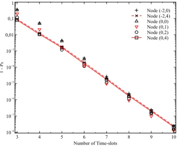
In Fig. 7, we consider the broadcast scenario in a regular line network of 9 nodes in which 𝑚𝑖𝑗 = 0.5 and 𝑑 = 100m. To better illustrate the results, 1 − 𝑃𝐵 is considered instead of 𝑃𝐵. We can see from the figure that for𝐾 < 5 time-slots, node 5 is the best broadcaster as its 1 − 𝑃𝐵 is minimum. However, when 𝐾 > 6, the preferable position to broadcast a message to the whole network is node 2. Furthermore, when the given relaying time-slots is increased, choosing a different broadcaster does not yield much better performance.
Fig. 6. Performance of the unicast scenario in a grid network of55 nodes, comparing to a line network of11 nodes.
Fig. 7. Performance of broadcasting in a regular line network of9 nodes, with different broadcasters.
In a grid of 45 nodes with 9 nodes in each row, 𝑚𝑖𝑗 = 0.5, 𝑑 = 100m and 𝑟 = 50m, the results in Fig. 8 suggest similar remarks as in Fig. 7. For 𝐾 < 5 time-slots, the best broadcaster is node (0, 4), the central node. Yet for 𝐾 > 6, node (0, 1) is in the better position to broadcast a message to the whole network while (0, 4), the node at the center of the network, is among the worst broadcasters. For example, with10 time-slots, the resulting sequence to broadcast to the whole network is{(0,1), (0,1), (0,1), (0,1), (0,2), (0,6), (2,7), (-1,7), (0,7), (1,7)}, starting from node (0,1), whose position is near the edge of one side of the network, rebroadcasts in a few time-slots at first and the later time-slots are used by distinct relay nodes on the other side of the network. On the
Fig. 8. Performance of broadcasting in a grid network of 45 nodes, with different broadcasters.
other hand, if node (0, 4) wants to broadcast given 10 time-slots, the resulting option is {(0,4), (0,4), (0,2), (0,6), (-1,7), (1,7), (0,7), (1,1), (-1,1), (0,1)}, node (0, 4) repeats for one more time-slot and the sequence keeps going back and forth to both sides of the network.
V. CONCLUSIONS
In this paper, we have proposed and evaluated a low-complexity heuristic algorithm for online relay assignment, which is highly likely to minimize the probability of error at the targeted receiver(s) for unicast as well as broadcast. Numerical examples show that our algorithm yields solutions matching exhaustive search but using less complexity, such that relay assignments can be made online also in large net-works. The algorithm works for unicast as well as broadcast, and differs from existing work in that it does not separate source nodes, relay nodes and destination nodes into three disjoint sets, but assumes that all nodes can overhear each
other. This makes the results more generally applicable for all types of wireless networks.
REFERENCES
[1] A. Nosratinia, T. E. Hunter, and A. Hedayat, “Cooperative communica-tion in wireless networks,” IEEE Commun. Mag., vol. 42, no. 10, pp. 74–80, 2004.
[2] A. Scaglione, D. L. Goeckel, and J. N. Laneman, “Cooperative com-munications in mobile ad hoc networks,” IEEE Signal Process. Mag., vol. 23, no. 5, pp. 18–29, 2006.
[3] A. Sendonaris, E. Erkip, and B. Aazhang, “User cooperation diversity. part i. system description,” IEEE Trans. Commun., vol. 51, no. 11, pp. 1927–1938, 2003.
[4] B. Rong and A. Ephremides, “Cooperative access in wireless networks: stable throughput and delay,” IEEE Trans. Inf. Theory, vol. 58, no. 9, pp. 5890–5907, 2012.
[5] T. Han and N. Ansari, “Heuristic relay assignments for green relay assisted device to device communications,” in Proc. IEEE Global Commun. Conf. 2013, Atlanta, GA, Dec. 2013, pp. 468–473. [6] K. Xie, J. Cao, X. Wang, and J. Wen, “Optimal resource allocation for
reliable and energy efficient cooperative communications,” IEEE Trans. Wireless Commun., vol. 12, no. 10, pp. 4994–5007, 2013.
[7] D. Yang, X. Fang, and G. Xue, “HERA: An optimal relay assignment scheme for cooperative networks,” IEEE J. Sel. Areas Commun., vol. 30, no. 2, pp. 245–253, 2012.
[8] Y. Shi, S. Sharma, Y. T. Hou, and S. Kompella, “Optimal relay assignment for cooperative communications,” in Proc. ACM Int. Symp. Mobile Ad Hoc Netw. Comput. 2008, Hong Kong SAR, China, May 2008, pp. 3–12.
[9] H. Xu, L. Huang, C. Qiao, X. Wang, S. Lin, and Y.-e. Sun, “Shared relay assignment (sra) for many-to-one traffic in cooperative networks,” IEEE Trans. Mobile Comput., vol. 15, no. 6, pp. 1499–1513, 2016. [10] A. Willig and E. Uhlemann, “Deadline-aware scheduling of cooperative
relayers in TDMA-based wireless industrial networks,” Wireless Netw., vol. 20, no. 1, pp. 73–88, 2014.
[11] L.-N. Hoang, E. Uhlemann, and M. Jonsson, “An efficient message dissemination technique in platooning applications,” IEEE Commun. Lett., vol. 19, no. 6, pp. 1017–1020, 2015.
[12] ——, “A novel relaying scheme to guarantee timeliness and reliability in wireless networks,” in Proc. IEEE Global Commun. Conf. Wksp., Washington, DC, Dec. 2016.
[13] M. K. Simon and M.-S. Alouini, Digital communication over fading channels. John Wiley & Sons, 2005, vol. 95.
[14] M. C. Robini and P.-J. Reissman, “From simulated annealing to stochas-tic continuation: a new trend in combinatorial optimization,” J. Global Optimization, vol. 56, no. 1, pp. 185–215, 2013.
[15] D. Jiang, Q. Chen, and L. Delgrossi, “Optimal data rate selection for vehicle safety communications,” in Proc. ACM Int. Wksp. Veh. Inter-netw. Syst. Applicat., San Francisco, CA, Sep. 2008, pp. 30–38.