Implementing and Evaluating CPU/GPU Real-Time Ray Tracing Solutions

M

V¨aster˚as, Sweden

Bachelor Thesis in Computer Science

Implementing and Evaluating

CPU/GPU Real-Time Ray Tracing

Solutions

D

N

Afshin Ameri E.

Thomas Larsson

Abstract

Ray tracing is a popular algorithm used to simulate the behavior of light and is commonly used to render images with high levels of visual realism. Modern multi-core CPUs and many-multi-core GPUs can take advantage of the parallel nature of ray tracing to accelerate the rendering process and produce new images in real-time. For non-specialized hardware however, such implementations are often limited to low screen resolutions, simple scene geometry and basic graphical effects.

In this work, a C++ framework was created to investigate how the ray tracing algorithm can be implemented and accelerated on the CPU and GPU, respectively. The framework is capable of utilizing two third-party ray tracing libraries, Intel’s Embree and NVIDIA’s OptiX, to ray trace various 3D scenes. The framework also supports several effects for added realism, a user controlled camera and triangle meshes with different materials and textures. In addition, a hybrid ray tracing solution is explored, running both libraries simultaneously to render subsections of the screen.

Benchmarks performed on a high-end CPU and GPU are finally presented for various scenes and effects. Throughout these results, OptiX on a Titan X performed better by a factor of 2-4 compared to Embree running on an 8-core hyperthreaded CPU within the same price range. Due to this imbalance of the CPU and GPU along with possible interferences between the libraries, the hybrid solution did not give a significant speedup, but created possibilities for future research.

Contents

2.4.1 Interactive Ray Tracing . . . 14

2.4.2 Ray Tracing Hardware . . . 14

2.5 Ray Tracing Libraries . . . 15

2.5.1 Embree . . . 15 2.5.2 OptiX . . . 16 3 RayEngine 17 3.1 Scenes . . . 18 3.2 Camera . . . 18 3.3 GUI . . . 19 3.4 Rendering . . . 19 3.4.1 OpenGL . . . 19 3.4.2 Embree . . . 19 3.4.3 OptiX . . . 20 3.4.4 Hybrid . . . 20 3.5 Effects . . . 21 3.5.1 Shadows . . . 21 3.5.2 Reflections . . . 21 3.5.3 Refractions . . . 21 3.5.4 Ambient Occlusion . . . 21 4 Results 22 4.1 Code . . . 22 4.2 Images . . . 22 4.3 Benchmarks . . . 22 4.3.1 Sponza Scene . . . 23 4.3.2 Sibenik Scene . . . .ˇ 25

4.3.3 Glass Scene . . . 28 4.3.4 Hybrid Solution . . . 30 5 Conclusions 32 5.1 Implementation . . . 32 5.2 Performance . . . 32 5.3 The Future . . . 34 6 References 35 Appendix A Gallery 38

1 Introduction

During the last 50 years, the process of generating 2D images from geometric 3D scenes (rendering) has become a significant area of interest within computer science. Computer generated imagery is a big part of our modern culture and industry, and is widely employed in areas including entertainment, business, manufacturing, architecture and medicine. Therefore, rendering techniques must evolve to meet the growing demands of our society. Interest lies not only in producing images more quickly and efficiently, but also to deliver more accuracy and realism. Two techniques for generating images out of scene information are rasterization and ray tracing.

In recent years, specialized ray tracing libraries have been published by the leading hardware vendors along with documented APIs (Application Programming Interfaces). Examples include Intel’s Embree [1], NVIDIA’s OptiX [2] and AMD’s FireRays SDK [3], which allow programmers access to accelerated ray tracing ker-nels. This thesis work will investigate the differences between implementing the ray tracing algorithm on the CPU (Central Processing Unit ) and GPU (Graphics Pro-cessing Unit ) respectively, using such libraries. Given a typical PC, a small window resolution (800x600 pixels), basic shading techniques and a 3D scene containing up to 10,000 polygons, a real-time effect (30 frames per second and above) can be ex-pected when rendering entirely on the CPU with Embree [4]. It is however unclear how the performance of a GPU-based system would compare for identical scenes and hardware.

These libraries, while efficient, are targeted to operate on either the CPU or GPU, and the other component will thus remain largely unused in rendering-based applications. The ability to share the rendering workload between these two com-ponents is therefore an attractive concept and will be another aspect of this work. In theory, such a collaboration could allow larger window resolutions, additional graphical effects and/or more complex scenes to be ray traced while preserving a real-time framerate.

1.1

Research Questions

1. How can the ray tracing algorithm be implemented on the CPU and GPU respectively, using third-party libraries?

2. What are the performance differences between such implementations, while ray tracing various scenes?

3. Is there a performance gain when sharing the render workload between two ray tracing libraries running simultaneously?

1.2

Method

To answer the research questions, a practical approach will be used, based on imple-mentation and benchmarking. For investigating CPU- and GPU-based ray tracing, the libraries Embree and OptiX have been chosen, due to their usage in the pro-fessional industry, thorough documentation and popularity. Knowing that they will eventually be used in cooperation, it is first necessary to get a basic understand-ing behind their respective features and program flow. As such, the libraries will initially be installed separately in different projects before being merged into a com-mon solution. Finally, a testing framework will be constructed in C++ to evaluate the two libraries against several 3D scenes of varying complexities. A hybrid mode that renders subsections of the screen using both the CPU and GPU will also be constructed.

Due to the complexity of evaluating performance it is required to have a full understanding of the solutions being measured (the ray tracing libraries in this case) and the factors that could affect the result. For this reason the framework will be implemented from the ground up, rather than by re-using existing tutorial code. This not only gives a deeper understanding of how the libraries are used, but ensures that only the interesting parts are measured.

Benchmarking interactive scenes can be challenging, since the performance will largely depend on the current camera and object locations. For instance, looking up at the skybox where there are no objects will give a much higher framerate than having all the objects in the frame at once. As such, a consistent method must be chosen to measure all solutions in order to produce a fair result. A viable option is to have the camera moving in a predetermined path, showcasing various angles of the scene. When comparing the different framerates in this animation between the libraries, we can deduce what objects are the most intensive to render and from what angles.

For benchmarking, only CPUs and GPUs that are available on the consumer level will be targeted, this excludes specialized ray tracing hardware and products in higher price brackets. Additionally, having equally priced components gives a fair basis to draw conclusions from and will determine the cost of ray tracing on the CPU and GPU, respectively.

2 Background

In broad terms, computer graphics rendering can be split into two categories: Pre-rendered and real-time rendering (also commonly referred to as offline and online rendering, respectively). For media such as movies and commercials, images may be created long before being shown to the consumer (pre-rendered). In these cases, the performance of the rendering algorithm may not be the main focus, but rather the visual fidelity of the product. Here, highly complex and intensive algorithms are executed on specialized hardware and the tasks are usually split between multitudes of processors in rendering farms. Additionally, the results are often manually mixed and adjusted afterwards to create the optimal result, with respects to the stylistic, cinematic or practical choices of the artist. In real-time rendering on the other hand, the goal is to produce a new set of frames each second to achieve the illusion of movement in a scene. The main upside of this is the ability to create an interactive experience for the user, something that is impossible with pre-rendered images alone. While films in their final form are pre-rendered, the actual production pipeline benefits greatly from quicker rendering, since most of the once practical (non-digital) special effects are now replaced with computer generated imagery. In the animation industry, artists also often desire to get visual feedback of the final image as they are designing and laying out movements in a 3D scene [5]. Being limited to offline rendering will slow down this process and relying on a primitive approximation will give compromised results. In scientific research, using graphics to simulate data requires the system to stay updated with changes that may occur in the underlying data source [6]. On the other side of the spectrum, in video games, the player may move freely and explore the computer-generated world, and a stuttering framerate will detract from this experience. It is a fact that many people, both producers, researchers and consumers are dependent on high quality real-time graphics in their daily lives.

Creating real-time graphics is generally more technically challenging and many clever tricks must be put into use to produce acceptable results, while running smoothly on both high- and low-end hardware. Countless platforms are targets for real-time rendering, including personal computers, mobile phones, gaming consoles, smartwatches and virtual reality headsets. Producing high-quality graphics while maintaining a desirable framerate can therefore be more challenging than achieving realism, depending on the underlying hardware. In the last decade, free access to specialized graphics APIs and architectures for programmers such as OpenGL [7] and DirectX [8] has brought new innovations and helped further this area.

2.1

Rasterization

The term rasterization has been given a double meaning in the rendering community. It is both used to describe the general method of converting vector geometry into a raster format (pixels) and the specific process of projecting scene objects onto a frame buffer. The latter definition will be used in this paper. Rasterization is the most popular method used in real-time applications such as games to quickly produce images of varying complexity. Implementations work on a per-object basis, applying a shading function to each pixel within the primitives (triangles or quads) of the target mesh, often running via shader programs (shaders). However, this method cannot take the remaining scene into account without relying on specialized data, such as shadow- and environment maps. Notable graphical artifacts will appear when this data is lacking and features such as transparency and self-reflection cannot be created easily. Nonetheless, rasterization has enjoyed massive success due to its speed and flexibility.

GPUs, once heavily catered to the rasterization pipeline, are nowadays pow-erful parallel machines capable of running arbitrary code. This has allowed other algorithms to be implemented to utilize the many-core GPUs of modern PCs. Mean-while, the CPU, usually devoted to file handling, logic and mathematics, can also be used for rendering tasks.

2.2

Illumination Models

For any form of rendering, an illumination model must be chosen, determining how the objects in the scene react to light (or the absence of light) and to each other. Depending on the hardware limitations and the desired graphical style, one model may be more attractive than another.

Rasterization is limited to local illumination, a model for calculating shading based entirely on the individual polygons and the lights in a scene. This limitation gives a significant performance boost, but also compromised visual results. In the first 3D games, simple shading had to be done and the amount of light sources were usually limited to a few per level. Game designers therefore often had to rely on textures to give a richer feeling to the world and immerse the player, since heavy calculations were not a viable option. Eventually, developers and filmmakers started to use workarounds to imitate more sophisticated algorithms, at a cost of memory usage, flexibility and elegance in the solutions. Consider shadow maps, which are special buffers used to store the distance (depth) of objects from the perspective of each light [9]. This can be used to quickly render soft or hard shadows from any object. While this gives acceptable results, transparent objects cannot cast shadows properly and larger buffers must be used for higher quality shadows. Additionally, the rendering pipeline becomes more complicated, especially when additional effects are added. To gain more knowledge about the scene without bloating the code and using extra memory, another model must be used.

Global Illumination is a family of algorithms that simulate lighting based on knowledge of all objects in a scene and can therefore be more physically correct than local illumination [10]. Among these algorithms are ray tracing, path tracing, radiosity, photon mapping and more. To produce realistic results, it is not enough

to do calculations based on the lights in a scene, because real-life photons react to all objects they come across. This factor, indirect lighting, is crucial for producing convincing images through light bouncing and color bleeding effects. For instance, a purely diffuse object of a certain color will still cast that color onto nearby surfaces, to an extent. While these methods give more realism, the rendering time is greatly increased and this is generally not suited for real-time rendering.

2.3

Ray Tracing

Figure 2.1: The ray tracing algorithm visualized. Primary rays (red) are sent out from the camera (eye), creating additional secondary rays (blue) at the intersections. Ray tracing, proposed in 1968 by Arthur Appel [11], was mostly ignored outside the academics up to the 2000s. It is known for producing realistic images at a high computational cost and is largely inspired by nature.

In real life, light sources send out countless photons in the form of waves that bounce around until they run out of energy or get absorbed by an observer’s eye. This would be too intensive to simulate in a computer due to the sheer amount of waves a source sends out. Additionally, only a tiny fraction of these waves will ever reach an eye and get observed. The ray tracing algorithm reverses this by sending rays out from the camera, towards the objects in the scene and detecting the intersection points using mathematical formulas. Additional rays can then be sent depending on the properties of the intersected material and texture [12]. This allows for reflections, refractions, shadows and many other phenomena of nature to be accurately implemented with ease [13]. Effects generated by cameras may also be mimicked, such as depth of field and motion blur [14].

Despite this optimization of the natural process, ray tracing is still a computa-tionally demanding task and was originally not considered a practical solution or at the very least limited to pre-rendering usage. However, since the rays are largely independent and unaware of each other, it benefits greatly from parallelization. This has allowed modern implementations to take advantage of the increasing power of multi-core technology to speed up rendering significantly.

2.3.1 Scene Intersection

Given a basic pinhole camera, a ray is fired for each pixel in the image towards the scene. These primary rays are used to determine the visibility of any object in view, which is done via intersection tests. For scenes with multiple objects, it is necessary to perform an intersection test on each of them and continue with the one closest to the camera. If no object is hit, the pixel can be set to a background color or a sky image.

To represent a ray, an origin point O and direction vector D is needed. The origin is set to the camera’s position and the direction to a value depending on the camera rotation and the pixel’s relationship with the screen dimensions. A point P at a distance t across this ray is then defined using a parametric equation:

P = O + tD (2.1)

Any geometry with a line-intersection representation can be added into a ray tracer. Implicit surfaces are a perfect example of this, defined using a single function F (x, y, z) = 0. This is another advantage when comparing to rasterization, which is limited to polygons (and sometimes points or straight lines). While triangles may be used to approximate any complex surface, using mathematical formulas can give potentially infinite detail depending on the distance from the viewer.

Spheres are among the simplest shapes to test against a ray, making them a popular case for ray tracing. The points P on a sphere with center point C, a radius r fulfill the following equation:

|P − C|2− r2= 0 (2.2)

Substituting the P component with our ray equation and solving the resulting quadratic equation gives a solution for the intersection distance t on the following form:

t = − b ± √

b − 4ac

2a (2.3)

Without performing the square root or division, we can see at a glance whether the ray hits the sphere or not. If the value under the square root is lower than 0 then the equation gives no real solutions, meaning that the ray completely missed the sphere. A value of 0 means that we have one hit (grazing the surface) and larger than 0 that we have two hits (on each side of the sphere). This fact makes spheres an efficient bounding volume to quickly traverse the scene (see 2.3.4), since there are no heavy operations involved when the value of t is out of interest.

The following equations for popular shapes can be solved in a similar fashion: • Cylinder oriented along the ray p + vt and radius r:

(P − p − (v, P − p)v)2− r2= 0 (2.4)

• Plane, where p is a point on the plane and N is a normal vector (perpendicular to the surface):

(P − p) · N = 0 (2.5)

• Discs use the plane equation followed by another condition, using the center C and radius r:

|P − C| <= r (2.6)

While these formulas are convenient for rendering objects, truth is that most practical implementations of ray tracing still use triangles due to their ability to combine and construct any conceivable shape.

One possible method to intersect a triangle is to check it against a parallel plane and measuring the hit against the triangle corners (vertices). M¨oller and Trumbore propose a quick triangle intersection formula that does not rely on a traditional plane equation, but instead translate and skew it into a unit triangle at the origin to simplify calculations [15].

2.3.2 Shading Model

Figure 2.2: A basic scene ray traced using the shading formula2.7.

After the intersection has been calculated (and the ray actually hit an object), a surface shading algorithm is applied to create a final color that is stored in the pixel. This stage usually combines the surface texture color, material properties, light and world contribution into a single formula. A popular option for shading is using the Phong reflection model, originally proposed for use with local illumination [16]. Nonetheless, the ray tracing features can be incorporated into it to produce realistic results.

To start off, take the original Phong reflection model for a scene with one light source:

I = KaIa+ KdIdmax(N · L, 0) + KsIsmax((V · R)p, 0) (2.7)

Where

I = The final pixel color Ka= Material ambient color

Kd= Material diffuse color

Ks = Material specular color

Ia = World ambient lighting

Id = Light diffuse color

Is = Light specular color

N = Surface normal vector

L = The vector from the hit point to the light V = The vector from the hit point to the camera R = The direction of a perfectly reflected ray p = Shininess constant for the material

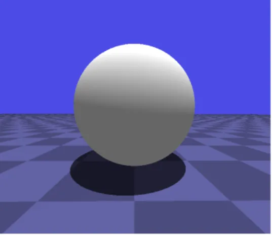
Figure 2.3: A basic scene ray traced using the shading formula 2.8. The shadows add a sense of depth and distance between the floor and sphere.

Figure 2.4: A basic scene ray traced using the shading formula 2.9. The sphere and blue background is reflected (mirrored) by the floor (Kr= 0.5).

As is typical with local illumination, the formula is oblivious as to whether there are objects blocking the light. With ray tracing however, we can cast an additional ray in the direction of the light and disregard its contribution if the ray intersects something (occluded ). This is known as a shadow ray (classified as a secondary ray) and replaces the shadow mapping method. Using the light contribution factor a (between 0 for fully occluded and 1 for no occlusion), the formula is as follows:

I = KaIa+ a(KdIdmax(N · L, 0) + KsIsmax((V · R)p, 0)) (2.8)

Similarly, we cast another ray in the direction of R to achieve realistic reflections [12]. In most implementations this is a recursive call, with the color of the ray added to the original pixel. However, not all material will be perfect mirrors, so there must be a way to weigh the reflection color by a factor. Given a material reflective factor Kr and a reflection result Rc, the formula is:

Figure 2.5: A basic scene ray traced using the shading formula 2.10. The rays continue to travel through the sphere while distorting the image slightly.

Figure 2.6: A basic scene ray traced using the shading formula2.11. The ambient occlusion effect adds a subtle shade below the sphere to accentuate the contact point with the floor.

Materials may also be transparent, in which case the light must continue traveling after the intersection. Depending on the material thickness, the ray will also be slightly bent, known as refraction [12] [17]. For instance, when traveling through water the ray will bend more than when traveling through glass. The contribution of this transmitted ray, Rt, will depend on the material transparency, Kt. The

ambient, diffuse and specular components must also be multiplied by its inverse to see through the material:

I = (1 − Kt)(KaIa+ a(KdIdmax(N · L, 0) + KsIsmax((V · R)p, 0))) + KrRc+ KtRt

(2.10) Ambient occlusion is a popular option for accurately simulating areas of the scene geometry where there is no light [18], for instance in creases, corners and

in holes. This adds a new level of realism to the resulting images by highlighting the shapes and contact points of the models through darker shadows (this effect is demonstrated in Figures 2.6 and A.4). To achieve this, a new batch of rays are sent in a hemisphere at the intersection point that is aligned to the normal vector, detecting occluded objects within a set radius. Increasing the number of rays will give higher quality ambient occlusion but add extra computations. To support ambient occlusion, the material contribution is typically multiplied by an occlusion factor o. This value is between 0 and 1 depending on the number of sample rays that intersected the scene.

I = o(1 − Kt)(KaIa+ a(KdIdmax(N · L, 0) + KsIsmax((V · R)p, 0))) + KrRc+ KtRt

(2.11) After these additions, this final formula can now be applied to create accurate shadows, reflections, refractions and ambient occlusion.

2.3.3 Ray Coherence

Primary rays are sent in similar directions, a property known as coherence. If a batch of rays hit the same object, the calculations can be accelerated using vec-torized instructions on either the CPU or GPU. Such optimizations can speed up performance dramatically and be crucial for real-time rendering. Secondary rays however, especially reflections and refractions on curved surfaces are usually inco-herent and slower to compute. Extra care must therefore be taken in these cases, for instance limit the amount of reflections and refractions in the scenes. Sorting the rays before calculations based on direction can also help solve this problem and ensure coherence, but may introduce extra overhead [19] [20].

2.3.4 Acceleration Structures

A ray tracer’s performance largely depends on the number of intersection tests per-formed. In a typical scene, millions of rays are sent out and many more to achieve basic effects such as shadows and reflections. An underlying spatial data structure must therefore be implemented to traverse the scene, serving to eliminate excessive intersection tests. Generally, the ray is first checked with an overlapping region of space covering the object(s) before going deeper and eventually checking the indi-vidual triangles.

Two popular acceleration structures are k-d trees and BVH (Bounding Volume Hierarchies) and are suited for different applications. k-d trees work by partitioning the scene in the same fashion as a binary tree, essentially halving the possible search space in each iteration. BVH will use an overlapping bounding volume for each object that does not require expensive intersection tests, for instance spheres.

Real-time ray tracing brings new challenges in this area, since the data structures must be updated each time objects are moved around or transformed [21]. This could cause additional performance drops and the acceleration structure must therefore be chosen with respect to these requirements. For instance, it has been shown that k-d trees are more suited for static scenes without moving objects [22], while BVH are preferred for dynamic scenes [23].

2.4

Related Work

With the increasing processing power of the last decade, ray tracing has garnered new interest in both academic fields, the industry and by hobbyist programmers. This section summarizes the most significant advancements in the field of ray tracing, with a focus on real-time rendering.

2.4.1 Interactive Ray Tracing

One of the first endeavors within real-time ray tracing was OpenRT, a scalable rendering engine introduced in 2002 [24]. At this point both static and dynamic environments could be ray traced at interactive speeds, relying on simple meshes and small window resolutions however. The engine offered an OpenGL-like API and was built on a client-server approach, allowing several connected hosts (CPUs) to render a single image. The project has since been abandoned, but remains as monumental point in the development of public real-time ray tracers.

As the technical landscape shifted from multi-processors towards single-processors with separate cores, new programming models had to arise to leverage the new par-allel paradigm. In 2006, Bigler et al. advocated a forward looking software architec-ture for interactive ray tracing based on this new way of computing [25]. Their ray tracing engine contains thread synchronization for efficient scaling with additional cores. They advocate the use of ray packets, SIMD instructions and ray coherence and discuss the new challenges that arise from interactive ray tracing.

At around the same time, Intel had started porting existing games to ray traced graphics on the CPU to demonstrate the feasibility of ray tracing in games. Quake 3 was initially ported, running at a framerate of 20 on a 512x512 resolution [26]. Later, in 2008, Enemy Territory: Quake Wars was ray traced, demonstrating realistic glass materials, water, better support for transparent textures among other things in the levels [27]. The framerates achieved ranged from 20 to 35 on a resolution of 1280x720.

Through the years, memory management remained as the primary bottleneck for GPU ray tracing, and explains why the focus remained on CPU-based solutions for so long. G¨unther and Popov et al. proposed k-d tree traversal and BVH-based packet traversal for real-time ray tracing on the GPU [28] [22]. Their new memory models eliminated the need for a stack on the GPU while traversing a scene, allowing performance greater than CPU counterparts. Memory management has since continued to evolve with regards to ray tracing and the GPU is now capable of efficient scene traversal and intersection tests in real-time.

2.4.2 Ray Tracing Hardware

Specialized ray tracing hardware has also been developed, the first being RPU (Ray Processing Unit ) in 2005 by Woop et al. [29]. Inspired heavily by the GPU, it utilized a multi-level SIMD design and rendered images much faster than heavily optimized CPU solutions at the time. It strived to be fully programmable, much like the GPGPUs (General Purpose GPUs) of today.

Recently, mobile ray tracing has started to garner considerable attention. Hard-ware architectures for ray tracing on mobile devices has arrived, such as RayCore [30]

and SGRT [31], capable of competing with existing GPU ray tracers. PowerVR Ray Tracing is a similar platform for hardware accelerated rendering [32]. Using their OpenRL SDK, programmers can write ray tracing applications, heavily abstracted from the underlying mobile hardware [33].

2.5

Ray Tracing Libraries

In order to supply ray tracing services to graphics engineers and hobbyist program-mers, several ray tracing libraries have been published with documented APIs and built-in functionality for intersection tests, acceleration structures and scene man-agement. This project will focus on two of them: Intel’s Embree and NVIDIA’s OptiX.

2.5.1 Embree

Embree is a set of high performance ray tracing kernels developed at Intel, designed for many-core x86 CPUs [1]. It is open source and contains an API for program-mers to implement acceleration structures, intersection and occlusion tests into their graphics applications. Being rather low level, it is suitable for adding into existing renderers or use for single-ray tasks, such as collision detection.

Rays are spawned using the RTCRay datatype and tested against a scene using the rtcIntersect function, while rtcOccluded is used for shadow rays. After the function returns, different properties are assigned to the ray, including the instance, geometry and primitive that was hit, along with triangle coordinates and a precal-culated normal vector. From this point on, it is the programmer’s responsibility to perform appropriate shading functions and store the result in a buffer to be rendered. Advanced users may use a custom function to override the intersections to create custom shapes, such as implicit surfaces. A filter function may also be assigned to run code each time a ray intersects an object. For instance, when a shadow rays hits a semi-transparent surface a variable can be deducted rather than terminating the ray, essentially creating shadows of different shades.

For coherent rays, packets of size 4, 8 or 16 can be used via the RTCRay4, RTCRay8 and RTCRay16 datatypes (for the latter, a Xeon Phi coprocessor is required) along with their respective rtcIntersect/rtcOccluded functions. This enables SSE2 (Streaming SIMD Extensions 2 ), AVX (Advanced Vector Extensions), AVX2 or AVX512 to process several rays in parallel, speeding up intersection/occlusion tests considerably in some cases.

For quick traversal of static and dynamic scenes, BVH data structures are imple-mented by the library, largely hidden from the user. Additional features of Embree are built-in support for Bezi´er curves, motion blur, displacement maps and hair geometry.

2.5.2 OptiX

Unlike Embree, OptiX operates in a similar fashion as OpenGL, offering a pro-grammable pipeline for efficient ray tracing on the GPU [2]. Introduced by NVIDIA in 2010, it has enjoyed massive success due to its ease-of-use, accessibility and high performance.

Much like OpenGL shaders, OptiX uses the CUDA kernels to run ray tracing programs written in PTX (Parallel Thread Execution), their virtual machine assem-bly language within the CUDA architecture. The programs themselves are written in a C++ environment, but use CUDA features to handle variables and buffers, and are finally converted to PTX during compilation.

First off, a ray generation program is defined, running once per pixel and firing rays into the scene. For each object material in the scene, two programs are defined: Any hit and Closest hit. These programs run for all intersections that will occur and handle the shading based on the material properties. Each geometry must also have a program to define intersections and bounding boxes in order to support triangle meshes or custom shapes. Optionally, a miss program can be written, running code each time a ray misses all the objects in the scene, creating the possibility for a sky box.

In the programs, a ray payload is defined, carrying over custom data between the different stages in the pipeline. This allows more complex operations such as counting the number of rays, having transparent shadows or creating general purpose rays. The fundamental function of OptiX is rtTrace, recursively tracing a newly created ray using the CUDA stack and returning with its result.

There is also support for numerous acceleration structures, created using context-> createAcceleration. Examples include low/medium/high quality BVH, high qual-ity k-d trees for triangle meshes or no acceleration at all (which may give increased performance in special scenarios).

3 RayEngine

Figure 3.1: A screenshot of RayEngine.

This chapter outlines the features of RayEngine, the framework created to in-vestigate the ray tracing performance of Embree, OptiX and a hybrid solution. It was developed in Microsoft Visual Studio 2013 using C++, targeted for Windows platforms. The code base does not contain any Windows dependencies however and may be ported to Linux and Mac if desired. To run the program, a NVIDIA GPU capable of running CUDA is required.

To get acquainted with the ray tracing libraries, they were first installed outside the renderer in separate projects, which allowed greater control and understanding of their main characteristics. Finally, they were added into RayEngine as separate render modes (See 3.4) and synchronized to use the same resources and graphical effects, to essentially produce identical images. For the hybrid solution, it was crucial to not have a visible border between the image produced by each library, since a screen splitting method was used (See3.4.4). For benchmarking it was also necessary to have the same visual result to be able to draw valid conclusions regarding the performance.

Four ray traced effects were added: hard shadows, reflections, refractions and ambient occlusion, all of which can be customized in real-time using on-screen set-tings. This proved to be challenging however, considering the nature of the project. Since Embree and OptiX use wildly different program flows, the effects had to be implemented two times each, while ensuring that they created the same results on the CPU and GPU.

3.1

Scenes

Before benchmarking the solutions, three scenes were prepared, designed to test the different features of the ray tracer:

• Sponza scene (66K triangles)

Contains a 3D reconstruction of the Sponza palace in Dubrovnik, Croatia. This model will test shadows and ambient occlusion. See FigureA.1for a high resolution render.

• ˇSibenik scene (75K triangles)

Contains a 3D reconstruction of the ˇSibenik Cathedral in ˇSibenik, Croatia. This is a larger model with shadows, ambient occlusion and a single level of reflection. See FigureA.2for a high resolution render.

• Glass scene (95K triangles)

Features the Stanford bunny, the Utah teapot, various glass models, a torus knot with a mirror material and a textured floor. This scene contains many curved reflective and transparent surfaces and will evaluate the recursive capa-bilities of the ray tracing libraries. See FigureA.3for high resolution renders. All the scenes were created using third-party .obj and .mtl files that are loaded and transformed via code. For simplicity, the objects are static and only triangle meshes are supported. The following C++ code snippet demonstrates how the Glass scene was constructed using translation and scaling:

S c e n e ∗ g l a s s S c e n e = r a y E n g i n e . c r e a t e S c e n e ( ” G l a s s ” , ” img / s k y . j p g ” , { 0 . 4 f } ) ; g l a s s S c e n e −>a d d L i g h t ( { 1 0 0 . f , 1 0 0 0 . f , 1 0 0 . f } , { 1 . f , 1 . f , 1 . f } , 1 0 0 0 0 . f ) ; g l a s s S c e n e −>l o a d O b j e c t ( ” o b j / f l o o r . o b j ” ) ; g l a s s S c e n e −>l o a d O b j e c t ( ” o b j / G l a s s / G l a s s P a c k . o b j ” ) −>s c a l e ( 0 . 1 f ) ; g l a s s S c e n e −>l o a d O b j e c t ( ” o b j / t e a p o t / t e a p o t . o b j ” ) −>s c a l e ( 0 . 3 f ) −>t r a n s l a t e ( { 2 0 . f , 0 . f , −40. f } ) ; g l a s s S c e n e −>l o a d O b j e c t ( ” o b j / bunny . o b j ” ) −>s c a l e ( 2 0 0 . f ) −>t r a n s l a t e ( { −30. f , −8. f , −40. f } ) ; g l a s s S c e n e −>l o a d O b j e c t ( ” o b j / TorusKnot / TorusKnot . o b j ” ) −>s c a l e ( 2 . 5 f ) −>t r a n s l a t e ( { −10. f , 1 0 . f , 4 0 . f } ) ;

Each scene supports a sky box texture, creating a more realistic environment. When a ray misses all objects, rather than terminating with a solid color the ray direction vector is transformed into a texture coordinate and used to fetch a color from an image.

3.2

Camera

The scenes are viewed from a virtual camera that can be controlled via code or by the user (See AppendixBfor controls). For the benchmarking stage, an animation was created for each scene to test the real-time capabilities. In this animation, the camera moves in a predetermined path, either in a circle, a straight line or stationary while looking around. It was not enough to render from a single viewpoint as different

perspectives of the scene would require more or fewer rays for the various effects. Similarly, randomly moving the camera around would not give a fair result between the libraries.

3.3

GUI

Since the framework holds many rendering features, it was necessary to isolate them when benchmarking and note the results. For instance, if a certain effect caused a massive performance drop, it was only by deactivating it that we could accurately measure the other effects. For this reason, a GUI (Graphical User Interface) was constructed that offers numerous settings that can be changed during runtime using the arrow keys. Examples of such settings include window size, which library to use, what scene to render, what effects to use and their intensity. Being able to change the render properties during runtime proved to be extremely helpful when locating performance issues, especially with the hybrid solution. See Appendix B for a full list of settings. The GUI also contains other useful information, such as the framerate and average rendering time for the different libraries.

3.4

Rendering

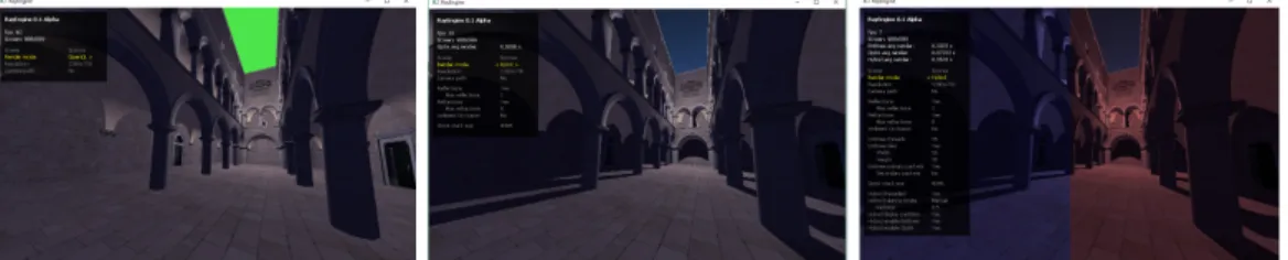
Figure 3.2: Three screenshots of the program, showing different render modes. From left to right: OpenGL, OptiX, Hybrid mode (half screen is Embree, other half OptiX). New settings are revealed in the GUI for different renderers.

Four render modes are available that can be switched during runtime using the settings menu: OpenGL, Embree, OptiX and Hybrid.

3.4.1 OpenGL

Scenes can first be rendered using OpenGL rasterization with shaders and basic Phong shading, offering (unsurprisingly) a much higher framerate than the ray trac-ers. This mode serves two purposes: First, it can be used to quickly position the camera when the ray tracing modes are too intense. Secondly, it can be used as a debugger for triangle meshes and for previewing object placements in the scenes.

3.4.2 Embree

With Embree being selected, the program enables ray tracing and performs all calcu-lations on the CPU. To share the workload between the available cores, the OpenMP

library is used [34]. RayEngine will split up the image into tiles that are then dis-tributed across all available cores to be rendered individually. The dimensions of the tiles (width and height) can be changed via the settings.

For primary rays, packets of size 8 are used, while single-rays are used for the (incoherent) secondary rays. This has shown to give a speedup compared to using packets for both primary rays and secondary rays, and may also be changed in the settings menu.

3.4.3 OptiX

With OptiX enabled, the entire screen is sent each frame to the CUDA kernels to be processed using the context->launch function. The GPU will then split up the workload accordingly and write the result to a texture that is rendered on the screen as two triangles. For memory optimization, the OpenGL resources are shared with OptiX, including triangle mesh data, material textures and output buffer texture. This is achieved using the functions context->createBufferFromGLBO and context->createTextureSamplerFromGLImage, telling the library to point the data source to an existing OpenGL VBO (Vertex Buffer Object ) or texture.

3.4.4 Hybrid

The hybrid mode utilizes both Embree and OptiX to render parts of the screen. By default, the left half is rendered by Embree, while the right half is sent to OptiX, giving a 50/50% split. A setting is available that displays these two partitions in different colors (blue for Embree, red for Optix, see Figure 3.2). This ratio can be changed manually or by a balancing algorithm that compares the render time of each component and adds/removes pixels accordingly. For instance, if Embree takes twice as long to render as OptiX, the algorithm will give 33% of the screen to the CPU, and 66% to the GPU.

In the implementation, the libraries are running on separate threads, once again using OpenMP. It is therefore important to have proper balancing, since both threads must finish at around the same time to achieve minimal waiting. Progressive ren-dering for OptiX was also explored using context->launchProgressive. In this case, OptiX sends rendering instructions to the GPU and waits for the result asyn-chronously. During this waiting, the Embree half is rendered on the CPU, all on the same thread. This led to conflicts with OpenGL however and did not yield any significant speedups. Additionally, there was no way to accurately measure the rendering time for the GPU during progressive rendering, making the balancing al-gorithm unusable. For these reasons the progressive rendering was discarded, but remains as an option in the code.

3.5

Effects

3.5.1 Shadows

Before adding the light contribution, a shadow ray is sent, checking for objects block-ing the light. This produces perfectly sharp/hard shadows, which is typical for ray tracing. More shadow rays can potentially be added to the code to produce a softer transition between darkness and light. When transparent objects are occluding the pixels, the shadows react accordingly.

3.5.2 Reflections

For realistic reflections, additional rays are cast in a Whitted style [12] and calculated by Embree via recursive calls and by OptiX via rtTrace. A setting is available that limits the amount of recursion, which is essential to avoid stack overflow on the CPU and potential crashes for parallel mirrored surfaces. As described in 2.3.2, each material has a factor that determines the contribution of this ray in the final color. For the torus knot object in the Glass scene, this value is 1, while a lower value is used for the ˇSibenik floor to blend the reflection with the texture.

3.5.3 Refractions

Transparent materials need to have the ray pass through it, while also contributing to the final color. This posed several design questions to the code structure. In the end, it was decided that transparent textures will cast an additional ray at the hit position, that may be bent depending on the index of refraction [17]. This creates interesting effects for glass materials (See FigureA.3), but adds extra computation images with a lot of transparent surfaces.

3.5.4 Ambient Occlusion

Ambient occlusion may be enabled via the settings menu to highlight the shapes of the objects in the scene through extra shadows. The amount of samples can also be adjusted for higher/lower quality of the darkened regions (in the benchmarks, 0, 9 and 25 samples are compared). Similarly, the radius of the hemisphere can be changed, which leads to different graphical effects and atmospheres in the scenes.

The ambient occlusion effect could potentially be swapped for soft shadows while achieving the same framerates, since they use similar methods of batch ray casting. One could argue however that soft shadows are quicker to calculate, since they are generally more coherent.

4 Results

4.1

Code

The code and executable of the framework can be found on GitHub [35]. See Ap-pendixBfor a full list of key commands and descriptions of the on-screen settings.

4.2

Images

See AppendixA for high resolution renders.

4.3

Benchmarks

To evaluate the solution, a set of benchmarks were designed to stress-test the features of RayEngine and compare the two libraries. As is typical with computer graphics, the framerate (FPS, Frames Per Second ) will be main interest to measure the real-time rendering capabilities.

For the following benchmarks, an Intel i7-5960X Extreme 8-core CPU (16 logical cores with hyperthreaded enabled) and a NVIDIA GeForce GTX Titan X GPU was used for running Embree and OptiX, respectively. All experiments were done on Windows 7 64-bit with 16GB RAM. Three scenes were evaluated: Sponza, ˇSibenik and Glass while ray tracing various effects.

In each test, a 300 frame animation was constructed that moves the camera around and displays varying angles of the scene. For each frame, the time taken to render (in seconds) was stored in a file. Note that this measurement only covers the actual ray tracing, not any overhead introduced from window operations or file writing. To calculate the FPS of each frame, the formula 1/t was used, where t is the render time. This will give a value corresponding to how many times this frame can be rendered in one second, given that the camera stays stationary. Each scene was tested using Embree and OptiX, three effect setups and three different render resolutions: 800x600, 1280x720 and 1920x1080 pixels (Full HD). This brings a total of 18 tests per scene, summarized in the following sections.

BVHs were used to accelerate both Embree and OptiX (in OptiX’s case, a Sbvh builder and Bvh traverser was used) to give a fair comparison. All tests also included a single light source and hard shadows, achieved by sending single-rays towards the light.

4.3.1 Sponza Scene

Figure 4.1: From left to right: Frame 0, 75, 150 and 225 in the Sponza animation. The Sponza scene contains no reflections and was therefore primarily a subject of primary- and shadow rays. To investigate the limits of occlusion tests using Embree and OptiX, ambient occlusion was also enabled with different sample sizes:

1. No ambient occlusion

2. Ambient occlusion with 9 samples 3. Ambient occlusion with 25 samples

Figure 4.3: Sponza scene performance with hard shadows and 9 ambient occlusion samples.

Figure 4.4: Sponza scene performance with hard shadows and 25 ambient occlusion samples.

Figure 4.5: Summary of Sponza scene performance.

4.3.2 Sibenik Sceneˇ

Figure 4.6: From left to right: Frame 0, 75, 150 and 225 in the ˇSibenik animation. The ˇSibenik scene, with its shiny floor was an experiment of how Embree and OptiX would perform given a single level of reflection. The animation proved to give extremely varying results. For instance, at frame 75 the camera looks straight into a door, giving us much less rays to compute than others, like frame 225. Interestingly, this moment was the only time in this scene that Embree outperformed OptiX at a small window resolution (800x600). Again, three levels of ambient occlusion were tested:

1. No ambient occlusion

2. Ambient occlusion with 9 samples 3. Ambient occlusion with 25 samples

Figure 4.7: ˇSibenik scene performance with hard shadows.

Figure 4.8: ˇSibenik scene performance with hard shadows and 9 ambient occlusion samples.

Figure 4.9: ˇSibenik scene performance with hard shadows and 25 ambient occlusion samples.

4.3.3 Glass Scene

Figure 4.11: From left to right: Frame 0, 75, 150 and 225 in the Glass animation. This final scene contained intensive recursive calls from reflections and refrac-tions. Here, the refractive glass caused major slowdowns, even though the refractive recursion was limited to 8 iterations. In frame 150, this limitation becomes appar-ent as the rays cannot penetrate all the glass objects and return with a black color. Regardless of this limit, the framerate drops dramatically in all test cases. Another intensive spot is frame 250 where the semi-transparent reflective teapot covers the entire screen. This fires as many refraction and reflection rays as there are primary rays.

Rather than using ambient occlusion, varying levels of reflection were investi-gated:

1. No reflections

2. 1 reflection (in this case, the reflection of the torus knot will not be a mirror) 3. 2 reflections (both the torus knot and its reflection will be a mirror)

Figure 4.13: Glass scene performance with hard shadows, 1-level reflections and 8-level refractions.

Figure 4.14: Glass scene performance with hard shadows, 2-level reflections and 8-level refractions.

Figure 4.15: Summary of Glass scene performance.

4.3.4 Hybrid Solution

Finally, all three scenes were tested using the hybrid solution. In the pure Em-bree/OptiX solutions (where the entire screen was rendered using one library) the ray tracer performed as expected. However, when allocating a subsection of the screen (from 25/75% to 75/25%) to either library, the performance could not exceed the OptiX-only solution. The scenes were rendered with 1-level of reflection, without ambient occlusion and in HD resolution from a single viewpoint.

Figure 4.16: Summary of hybrid performance when the screen is split between the CPU (Embree) and GPU (OptiX) in different partitions.

5 Conclusions

This project gave a thorough understanding about the interfaces and relative per-formance of two popular ray tracing libraries, Embree and OptiX, operating on a high-end CPU and GPU. Several ray tracing effects were also researched, imple-mented and measured: Hard shadows, reflections, refractions and ambient occlusion. However, new questions were also raised regarding the cost of ray tracing on the CPU/GPU and whether two separate ray tracing libraries running simultaneously is a feasible option for achieving higher framerates.

5.1

Implementation

Coding wise, installing the two libraries were two vastly different experiences. Us-ing Embree, it was not obvious how to achieve maximum performance and many different strategies were tested. For instance, one initial idea was to trace each ray category separately (eg. first all the primary rays, then all shadow rays, followed by all reflection rays...) and finally compile the results. However, this caused addi-tional overhead from the data structures required and slowed down the performance compared to other methods. Finally, it was decided to settle for a tiled approach, using packets for primary rays and single secondary rays.

OptiX required a more elaborate setup before rendering, taking up more than twice the amount of code compared to Embree. All the scenes and objects had to be carefully initialized with their respective programs, variables and buffers. However, the actual rendering implementation went much smoother, largely thanks to the heavy abstraction of the OptiX pipeline and its similarities with OpenGL.

All in all, since Embree is at such a low level and open-source it can be used for many different purposes, not necessarily rendering related. OptiX is a strong contrast to this, tailored to be used as an entire rendering engine for fast ray traced graphics. While it is customizable using variables, buffers and ray payloads, its backend and inner mechanisms are largely hidden from the user.

5.2

Performance

Measuring CPU vs. GPU performance is a big challenge, due to the inherent dif-ferences between the two architectures. They are designed from the ground up for specific tasks and performance drops is to be expected when putting them out of their ”comfort zones”. There is therefore no such thing as a CPU and GPU with equal performance, since it varies considerably based on the task being measured. The GPU, with its hundreds of cores and thousands of threads is tailored for rapid concurrent vector and matrix operations. In contrast, the CPU only has a few pow-erful cores suitable for running an operating system: Managing a few applications in parallel, scheduling and performing file operations.

Due to the massive parallelism of the GPU, it can therefore be assumed to always give better ray tracing performance. However, if this was the case, CPU ray tracing (researched by Intel among others) would be considered ludicrous. In fact, Intel promises 40-70% better performance when running Embree on a Intel Xeon Phi preprocessor against OptiX on a Titan X [2]. Their results were however based on components within entirely different price brackets. At this time, their Xeon Phi can be ordered for around $2000, while a Titan X lies at $1300. At the consumer level, a Titan X is more accessible in this case and the CPU result becomes less interesting.

Throughout my benchmarks, OptiX on a Titan X performed better by a factor of 2-4 compared to Embree running on an 8-core hyperthreaded CPU within the same price range (around $1300). OptiX could process a large amount of reflections, shad-ows or ambient occlusion in HD, while preserving a real-time framerate. Meanwhile, Embree could barely keep up and mostly remained below the 20 FPS mark. A few exceptions exist, for instance when the window size is small, the visible geometry is simple and there are no reflections (see Figure4.7). Embree also performed slightly better under extreme circumstances where there was barely a real-time effect for either cases (see Figure4.14). The framerate of Embree is also revealed to be more stable by the charts, forming a rather smooth line compared to OptiX.

There are possibilities for speeding up Embree, for instance using Intels SPMD Program Compiler (ISPC), which is said to give a performance boost of up to 10% when rendering [36]. Also, other threading mechanisms could be explored other than OpenMP, such as Intels Threading Building Blocks (TBB) [37]. The scenes consisted of static objects, and updating their transformations could also potentially be quicker on the CPU than the GPU. It is however unclear if these factors would add up enough to beat OptiX at real-time rendering for this setup.

The hybrid solution also suffered due to this imbalance, failing to give a signif-icant speedup when allocating differently sized partitions on the CPU and GPU. Other factors could also come into play here. For instance, it is not known for sure whether OptiX is strictly GPU based. If OptiX uses the same processing re-sources as Embree, the threading mechanisms could suffer and cause a slowdown. In fact, running the OptiX renderer of RayEngine while checking the Windows Task Manager reveals a higher CPU usage percent than when running in OpenGL mode. Given the current implementation, 3D scenes and hardware, a better CPU is required to meet the ray tracing performance of OptiX, which will not be cheap. From these results it seems like CPU based ray tracing is more expensive overall when compared to the GPU for identical scenes. Considering the massive parallelism of the GPU and its speciality in graphics related calculations, this is no surprise. On top of this, NVIDIA recently released their next line of graphics hardware, promising up to 3 times performance for higher resolutions and at similar price ranges as the previous generation [38]. It will be interesting to find out how they can handle ray tracing compared to the Titan X for these scenes.

5.3

The Future

For future work on RayEngine, OptiX should be replaced with (or accompanied by) a lower level CUDA-based solution to gain larger control over the GPU rendering process and memory management. At this point, it is unclear whether OptiX is using CPU resources while rendering, considering that the hybrid solution is not giving optimal performance while both Embree and OptiX are running on separate threads. Many other ray tracing effects can also be explored to push the limit of what is possible to process in real-time. Due to time constraints, animated objects and lights were not implemented either. If added, their effect on the rendering performance from updating the acceleration structures could then be compared for the different libraries.

Real-time ray tracing, still in its infancy, has a long way to go before becoming a viable option for the average consumer. New innovations still await in this area, both on the software and hardware side, and ray tracing will undoubtedly come to replace rasterization completely in future real-time graphics applications. It is only a matter of time before we will have the processing power necessary to ray trace convincing images at high resolutions, while maintaining interactivity with the user.

6 References

[1] Ingo Wald et al. “Embree: A Kernel Framework for Efficient CPU Ray Trac-ing”. In: ACM Transactions on Graphics (TOG) 33.4 (2014), p. 143.

[2] Steven G Parker et al. “Optix: A General Purpose Ray Tracing Engine”. In: ACM Transactions on Graphics (TOG) 29.4 (2010), p. 66.

[3] AMD. FireRays SDK. http : / / developer . amd . com / tools - and - sdks / graphics- development/firepro- sdk/firerays- sdk/. Accessed: 2016-06-09. 2016.

[4] Yvonne Schudeck. “Ray traced gaming, are we there yet?” B.S. Thesis. IDT: M¨alardalens H¨ogskola V¨aster˚as, Feb. 2016.

[5] Pixar NVIDIA GPU Feature Film Production Keynote.http://on-demand. gputechconf.com/gtc/2014/video/S4884-keynote-nvidia-gpu-feature-film-production-pixar.mp4. Accessed: 2016-06-09. May 2014.

[6] L Miguel Encarnacao et al. “Future Directions in Computer Graphics and Visualization: From CG&A’s Editorial Board”. In: Computer Graphics and Applications, IEEE 35.1 (2015), pp. 20–32.

[7] OpenGL The Industry’s Standard for High Performance Graphics. https : //www.opengl.org/. Accessed: 2016-06-09. 2016.

[8] Microsoft. DirectX. https : / / support . microsoft . com / enus / kb / 179113. Accessed: 2016-06-09. 2016.

[9] Randima Fernando. “Percentage-closer soft shadows”. In: ACM SIGGRAPH 2005 Sketches. ACM. 2005, p. 35.

[10] Per H Christensen. “Point-based global illumination for movie production”. In: ACM SIGGRAPH. 2010.

[11] Arthur Appel. “Some techniques for shading machine renderings of solids”. In: Proceedings of the April 30–May 2, 1968, spring joint computer conference. ACM. 1968, pp. 37–45.

[12] Turner Whitted. “An improved illumination model for shaded display”. In: ACM Siggraph 2005 Courses. ACM. 2005, p. 4.

[13] Bram De Greve. “Reflections and refractions in ray tracing”.http://users. skynet.be/bdegreve/writings/reflection_transmission.pdf. Accessed: 2016-06-09. Nov. 2006.

[14] Qiming Hou et al. “Micropolygon ray tracing with defocus and motion blur”. In: ACM Transactions on Graphics (TOG). Vol. 29. 4. ACM. 2010, p. 64. [15] Tomas M¨oller and Ben Trumbore. “Fast, minimum storage ray/triangle

[16] Bui Tuong Phong. “Illumination for computer generated pictures”. In: Com-munications of the ACM 18.6 (1975), pp. 311–317.

[17] LH Nelken. “Index of refraction”. In: IN: Handbook of Chemical Property Es-timation Methods: Environmental Behavior of Organic Compounds. American Chemical Society, Washington, DC. 1990. p 26. 1-26. 21. 7 tab, 16 ref. (1990). [18] Michael Bunnell. “Dynamic ambient occlusion and indirect lighting”. In: Gpu

gems 2.2 (2005), pp. 223–233.

[19] Kirill Garanzha and Charles Loop. “Fast Ray Sorting and Breadth-First Packet Traversal for GPU Ray Tracing”. In: Computer Graphics Forum. Vol. 29. 2. Wiley Online Library. 2010, pp. 289–298.

[20] Christian Eisenacher et al. “Sorted deferred shading for production path trac-ing”. In: Computer Graphics Forum. Vol. 32. 4. Wiley Online Library. 2013, pp. 125–132.

[21] Ingo Wald et al. “State of the art in ray tracing animated scenes”. In: Computer Graphics Forum. Vol. 28. 6. Wiley Online Library. 2009, pp. 1691–1722. [22] Stefan Popov et al. “Stackless KD-Tree Traversal for High Performance GPU

Ray Tracing”. In: Computer Graphics Forum. Vol. 26. 3. Wiley Online Library. 2007, pp. 415–424.

[23] Niels Thrane and Lars Ole Simonsen. “A comparison of acceleration structures for GPU assisted ray tracing”. MA thesis. Aug. 2005.

[24] Andreas Dietrich et al. “The OpenRT Application Programming Interface– Towards a Common API for Interactive Ray Tracing”. In: Proceedings of the 2003 OpenSG Symposium. Citeseer. 2003, pp. 23–31.

[25] James Bigler, Abe Stephens, and Steven G Parker. “Design for parallel interac-tive ray tracing systems”. In: Interacinterac-tive Ray Tracing 2006, IEEE Symposium on. IEEE. 2006, pp. 187–196.

[26] J¨org Schmittler et al. “Realtime ray tracing for current and future games”. In: ACM SIGGRAPH 2005 Courses. ACM. 2005, p. 23.

[27] Daniel Pohl. “Light It Up! Quake Wars Gets Ray Traced”. In: Intel Visual Adrenaline 2 (2009), pp. 34–40.

[28] Johannes G¨unther et al. “Realtime ray tracing on GPU with BVH-based packet traversal”. In: Interactive Ray Tracing, 2007. RT’07. IEEE Symposium on. IEEE. 2007, pp. 113–118.

[29] Sven Woop, J¨org Schmittler, and Philipp Slusallek. “RPU: a programmable ray processing unit for realtime ray tracing”. In: ACM Transactions on Graphics (TOG). Vol. 24. 3. ACM. 2005, pp. 434–444.

[30] Jae-Ho Nah et al. “RayCore: A ray-tracing hardware architecture for mobile devices”. In: ACM Transactions on Graphics (TOG) 33.5 (2014), p. 162. [31] Won-Jong Lee et al. “SGRT: A mobile GPU architecture for real-time ray

trac-ing”. In: Proceedings of the 5th high-performance graphics conference. ACM. 2013, pp. 109–119.

[32] Imagination Technologies. PowerVR Ray Tracing. https : / / imgtec . com / powervr/ray-tracing/. Accessed: 2016-06-09. 2016.

[33] Imagination Community. PowerVR OpenRL SDK. https : / / community . imgtec . com / developers / powervr / openrl - sdk/. Accessed: 2016-06-09. 2016.

[34] Leonardo Dagum and Rameshm Enon. “OpenMP: an industry standard API for shared-memory programming”. In: Computational Science & Engineering, IEEE 5.1 (1998), pp. 46–55.

[35] David Norgren. RayEngine on GitHub.https://github.com/DavidNorgren/ RayEngine. Accessed: 2016-06-09.

[36] Matt Pharr and William R Mark. “ISPC: A SPMD compiler for high-performance CPU programming”. In: Innovative Parallel Computing (InPar), 2012. IEEE. 2012, pp. 1–13.

[37] Chuck Pheatt. “Intel threading building blocks”. In: Journal of ComputingR

Sciences in Colleges 23.4 (2008), pp. 298–298.

[38] NVIDIA. GeForce GTX 1080.http://www.geforce.com/hardware/10series/ geforce-gtx-1080. Accessed: 2016-06-09. June 2016.

A Gallery

Figure A.1: The Sponza scene with shadows and ambient occlusion.

Figure A.3: Different angles of the Glass scene. The rays are bent as they travel through the glass, distorting the image behind.

Figure A.4: A car model ray traced at interactive framerates. The ambient oc-clusion (second image) reveal the rims and adds a second shadow below the car in exchange for a lower framerate.

B Controls & Settings

This section serves as a manual for controlling RayEngine and changing the settings. See the GitHub page in case new settings have been added [35].

To start off, the camera is oriented by left clicking and moving the mouse around. While the left button is pressed, the following key commands become active:

• W/S/A/D

Move forward/back/left/right. • Q/E

Roll the camera. • Space/Shift

Speed up/Slow down movement. • T/G

Increase/Decrease FOV (Field of View ). The following key commands are also available: • F1

Show/Hide GUI. • F2

Start/Stop benchmarking. • F3

Save a HD screenshot into the renders/ folder.

The up/down arrow keys are used to navigate through the settings menu, while right/left will change the selected value. Here are short descriptions of the settings:

• Scene

Changes the current scene from the ones pre-loaded into memory. • Render mode

Switches the render mode between OpenGL, Embree, OptiX and Hybrid. • Resolution

Switches the window resolution between 800x600, 1280x720 and 1980x1080. • Camera path

• Reflections

Enables/Disables reflections in the scene. – Max reflections

Sets the maximum number of recursive calls for reflections. • Refractions

Enables/Disables refractions/transparent surfaces in the scene. – Max refractions

Sets the maximum number of recursive calls for refractions/transparent surfaces.

• Ambient Occlusion

Enables/Disables ambient occlusion in the scene. – AO samples

The amount of rays to send in a hemisphere around the intersection point. A larger value will give softer (less noisy) shades, but require more processing.

– AO radius

The radius of the sampling hemisphere. – AO power

The power/strength of the ambient occlusion effect. – AO noise scale

Determines the scale of the noise texture used when randomly sampling. • Embree threads

Tells OpenMP how many threads to use when Embree is rendering, this value is used with omp set num threads.

• Embree tiles

Enables/Disables tiles when Embree is rendering. If disabled, a single loop will be used.

– Width/Height

Determines the dimensions of the tiles. A value larger or equal to the packet size (8) is recommended to assure coherency.

• Embree primary packets

Packets (RTCRay8) will be used for all the primary rays. • Embree secondary packets

Packets will be used for all the secondary rays (shadows, reflections, refractions, ambient occlusion). This setting has shown to give a slowdown.

• OptiX progressive render

If enabled, progressive rendering will be used by OptiX, i.e. the program will use a non-blocking launch call.

• OptiX stack size

Sets the size of the GPU stack. A small value will lead to distorted reflections and refractions.

• Hybrid threaded

The hybrid mode will use a threaded approach, where the master approach runs OptiX while the other runs Embree. After both threads have finished, the result will be fetched and rendered on the screen.

• Hybrid balance mode

Changes the Hybrid balancing mode, either manual or based on the render time.

– Partition

When the balance mode is manual, this setting will determine the amount of the screen to give to Embree and OptiX, respectively.

• Hybrid Display Partition

When enabled, the Embree and OptiX images will be highlighted blue and red.

• Hybrid Enable Embree

Enables/Disables Embree. Used for debugging purposes. • Hybrid Enable OptiX