JUNCTION BASED ROUTING: A NOVEL TECHNIQUE FOR LARGE NETWORK ON CHIP PLATFORMS

1

JUNCTION BASED ROUTING:

A NOVEL TECHNIQUE FOR LARGE

NETWORK ON CHIP PLATFORMS

Shabnam Badri

THESIS WORK 2011

ELECTRONICS

2

JUNCTION BASED ROUTING:

A NOVEL TECHNIQUE FOR LARGE

NETWORK ON CHIP PLATFORMS

Shabnam Badri

This thesis work is performed at Jönköping Institute of Technology within the subject area Electronics. The work is part of the university’s two-year master’s engineering degree.

The authors are responsible for the given opinions, conclusions and results. Supervisors: Shashi Kumar and Rickard Holsmark

Examiner: Shashi Kumar

Credit points: 30 points (D-level)

Date:

Abstract

i

Abstract

To support communication among hundreds of cores on a chip, on-chip communication must be well organized. In the embedded systems using such a chip, the communication patterns can be profiled and routing can be well planned off-line. Source routing, with many advantages over distributed routing, will be very suitable in such contexts. However, source routing has one serious drawback of overhead for storing the path information in header of every packet. This disadvantage becomes worse as the size of the network grows. In this thesis we propose a technique, called Junction Based Routing (JBR), to remove this limitation. In the proposed technique, path information for only a few hops is stored in the packet header. With this information, either the packet reaches the destination, or reaches a junction from where the path information for on-ward path is picked up.

There are many interesting issues related to this approach. Two important issues related to JBR, namely, number and position of junctions and path computation for efficient deadlock free routing are discussed and solved in this thesis work. Increase in path length by using the minimum number of junctions, link load distribution while computing paths, path encoding for JBR and packet format in JBR are also discussed. A few tools have been developed in MATLAB to analyze the various aspects of JBR. A simulator has been also developed to evaluate the performance of JBR with simple source routing. Outline of the architecture for a junction is also proposed.

The results of simulation-based experiments show that the performance of JBR is similar to source routing. JBR is compared with source routing and the simulation-based results show that latency does not increase so much using junctions. Throughput also does not level off significantly. Header flit in JBR can carry payload data and this improves the performance of JBR in terms of throughput and latency compared to source routing which needs to store large path information. We observe improvement in throughput as compared to basic source routing when payload is very small.

Key Words

System on Chip (SoC) Core-Based Design On Chip Communication Network on Chip (NoC) Packet Switched Network Routing Algorithms Source Routing

Junction-Based Routing

Acknowledgement

ii

Acknowledgement

I am heartily thankful to my supervisor, Prof. Shashi Kumar, whose encouragement, guidance and knowledgeable support from the initial to the final level enabled me to do my final thesis. I am proud to record that I had the opportunity to work with an exceptionally experienced professor like him. I am indebted to him more than he knows.

Many thanks go to Rickard Holsmark for his valuable advice. He always kindly grants me his precious time even for answering some of my unintelligent questions.

I gratefully thank Alf Johansson for being always caring and I am thankful to all my teachers.

My family deserves special mention for their unconditional love and inseparable support.

Table of Contents

iii

Table of Contents

1

Introduction ... 1

1.1 SYSTEM ON CHIP ... 1

1.2 OPTIONS FOR INTERCONNECTING THE CORES IN A SOC ... 1

1.2.1 Point to Point Connections ... 1

1.2.2 Bus-Based System on Chip ... 2

1.2.3 Network on Chip (NoC)... 3

1.3 ISSUES IN NOC-BASED SOCDESIGN ... 3

1.3.1 Topology... 3

1.3.2 Routing Algorithms ... 3

1.4 PROJECT OBJECTIVES AND TASKS ... 4

1.5 THESIS LAYOUT... 5

2

Theoretical Background ... 6

2.1 NETWORK ON CHIP ... 6

2.2 TERMINOLOGY OF NOC ... 7

2.2.1 Network Architecture ... 7

2.2.2 Direct and Indirect Networks ... 7

2.2.3 Topology... 8

2.2.4 Network Diameter ... 8

2.2.5 Path ... 9

2.3 COMPONENTS OF NOC ... 9

2.3.1 Router... 9

2.3.2 Resource Network Interface (RNI) ... 9

2.4 SWITCHING ... 10

2.4.1 Circuit Switching ... 10

2.4.2 Packet Switching ... 10

2.5 BUFFERS AND VIRTUAL CHANNELS ... 11

2.6 ROUTING ... 12

2.6.1 Source vs. Distributed Routing ... 12

2.6.2 Deterministic vs. Adaptive Routing ... 12

2.6.3 Static vs. Dynamic Routing... 13

2.6.4 Minimal vs. Non-minimal Routing ... 13

2.6.5 Application Specific Routing ... 13

2.7 DEADLOCK-FREE ROUTING ALGORITHMS... 13

2.7.1 Deadlock, Livelock and Starvation ... 13

2.7.2 Turn-Model Routing Algorithms ... 14

2.8 EVALUATION OF NOC ... 16

2.8.1 Network Simulators ... 16

2.8.2 Performance Parameters ... 16

2.8.3 Traffic Types ... 18

3

Junction-Based Routing ... 19

3.1 AN ILLUSTRATION OF JUNCTION-BASED ROUTING ... 19

3.2 ANALYSIS OF JUNCTION-BASED ROUTING ... 20

3.2.1 Packet Format and Path Information ... 20

3.2.2 Header Overhead in JBR ... 22

3.3 CHALLENGES IN JBR ... 22

3.3.1 Number and Position of Junctions ... 23

3.3.2 A Case Study: Number and Position of Junctions ... 25

3.4 INCREASE IN PATH LENGTH BY USING JUNCTIONS ... 28

3.4.1 Calculating Extra Overhead of Increase in Path Length ... 28

Table of Contents

iv

3.5 JUNCTIONS AND DEADLOCK-FREE ROUTING ... 33

4

Path Computations for Mesh Topology NoC with Junctions

35

4.2 ANALYSIS OF JUNCTION-BASED NETWORKS USING DIFFERENT TURN-MODEL ROUTING ALGORITHMS... 36

4.2.1 Junction Configurations for North-Last Routing Algorithm ... 37

4.2.2 Junction Configurations for Other Kinds of Routing Algorithms ... 38

4.2.3 Comparison of Different Routing Algorithms Used ... 39

4.3 PATH SELECTION ... 40

4.3.1 Link Load Distribution ... 40

4.3.2 An Example of Selecting the Best Path for Each Communicating Pair ... 41

4.4 PACKET FORMAT IN JBR ... 43

4.4.1 Flit Types... 44

4.4.2 HEAD Flit ... 44

4.4.3 BODY Flit... 45

4.4.4 END Flit ... 46

4.4.5 Comparison of Two Different Header Flit Formats ... 46

4.5 PATHS ENCODING ... 46

4.6 ARCHITECTURE OF A JUNCTION-BASED ROUTER ... 48

4.6.1 Main Blocks of a Junction-Based Router ... 49

4.6.2 Arbitration and Control Unit ... 49

4.7 ADVANTAGES AND DISADVANTAGES OF JBR... 51

5

Performance Evaluation of JBR ... 52

5.1 PACKET DELAY MODEL FOR JBR ... 52

5.2 LANGUAGE USED FOR MODELING ... 53

5.3 SIMULATION OF JBR ... 54 5.3.1 RES_RNI_TYPE... 54 5.3.2 ROUTER_TYPE... 55 5.3.3 NetworkConfigurator ... 55 5.3.4 ControlStat ... 55 5.4 SIMULATION RESULTS ... 56 5.4.1 Evaluation of Performance of JBR ... 56

5.4.2 Performance Evaluation of Source Routing ... 59

5.4.3 Comparison of JBR and Source Routing ... 62

5.4.4 Importance of Smaller Routing Information ... 68

6

Conclusions ... 72

6.1 CONTRIBUTIONS AND RESULTS ... 72

6.1.1 Junction-Based Routing ... 72

6.1.2 Number and Position of Junctions ... 72

6.1.3 Increase in Path Length by Using Junctions ... 72

6.1.4 Path Computations for Mesh Topology Network on Chip with Junctions ... 73

6.1.5 Analysis of Junction-Based Networks Using Different Turn-Model Routing Algorithms 73 6.1.6 Link Load Distribution ... 73

6.1.7 Packet Format in JBR and Paths Encoding ... 74

6.1.8 Simulation of JBR ... 74

6.1.9 Simulation Results... 74

6.2 LIMITATIONS ... 74

6.3 FUTURE WORK ... 74

7

References ... 76

Table of Contents

v

8.1 NUMBER AND POSITION OF JUNCTIONS FOR DIFFERENT NETWORK SIZES AND DIFFERENT HOP COUNT LIMITS ... 78 8.2 JUNCTION CONFIGURATIONS FOR A 7X7MESH NETWORK AND A GIVEN HOP COUNT LIMIT OF 5

81

8.3 COMPARISON OF JBR AND SOURCE ROUTING FOR VARIOUS ROUTING ALGORITHMS IN LOCAL TRAFFIC ... 83

8.3.1 Latency Graphs... 83 8.3.2 Throughput Graphs ... 85

Introduction

1

1 Introduction

This thesis focuses on improvement of the communication between components of a system which is integrated on a single chip. In this chapter, we introduce the System on Chip and different methods for connecting components of the system. We will also introduce the area and problems handled in the thesis.

1.1 System on Chip

A core is an individual component that has a particular, often advanced, functionality. Today, it is possible to integrate a large number of cores (e.g. general purpose processors, embedded memories, DSP cores, FPGA blocks, I/O blocks, ASIC blocks, etc.) on a single silicon chip. Integrating the entire system on one chip reduces the size

and increases the performance of electronic systems. For example,

STMicroelectronics announced FLI7540, a new TV System-on-Chip lately. 1700+ DMIPS CPU with 256 KBytes of Level 2 cache offers a high performance TV [13]. These independent blocks can be of unequal size. Interconnecting pre-designed cores (resources) or IP-cores (Intellectual Property) becomes harder and harder by increasing the number of cores. Reducing design complexity and power consumption are some of the most important issues for SoC design [3].

Figure 1-1.FLI7540 - Digital TV System-on-Chip and Video-Enhancement IC (Photo from ST Website)

1.2 Options for Interconnecting the Cores in a SoC

Choosing a proper way for interconnecting the cores in a SoC design is an important step. A good interconnection reduces manufacturing cost and complexity. It decreases energy consumption as well. It also improves the performance of a system, for instance by decreasing communication delay between the cores [1][2].

1.2.1 Point to Point Connections

The first option for interconnecting the cores was to use direct point to point connections between cores, as illustrated in Figure 1-2.

Introduction

2

Figure 1-2.An Illustration of Direct Interconnect for On-Chip Communication

Main problems of this type of interconnection are that, it requires a lot of wires, I/O pins and big routing area and the system is not scalable. It is too hard to reuse this system and the routing resources are not utilized very well.

1.2.2 Bus-Based System on Chip

The basic idea is to share wires to connect several cores. Many of the existing SoCs are bus-based [3].

Figure 1-3.Bus-based System on Chip

A bus arbiter chooses a component to be granted bus access. Communication is fast, but bus access-time is increased by increasing the number of users. Speed of bus and the delay depend on the length of the bus and the longest physical distance between two resources, respectively. One pair can communicate to each other at a time and the cores compete for the bus. The hierarchical, segmented and pipelined buses are some of the advanced ways for bus-based systems. Shared buses may be suitable for systems with less than 8 resources and when the communication requirement is low on average, few resources are sources and the majority of resources are destinations [4].

Introduction

3

1.2.3 Network on Chip (NoC)

Network on Chip (NoC) has emerged as a dominant paradigm for synthesis of multi-core SoCs. As illustrated in Figure 1-4, in NoC paradigm, multi-cores are connected to each other through a network of routers and they communicate among themselves through packet-switched communication. A large number of different NoC architectures have been proposed by different research groups based on this paradigm [2][4]. Network topology and routing algorithm are the two most important aspects which distinguish various proposed NoC architectures. Router is the most important component for design of the communication back-bone of a NoC system (like any other network). In a packet switched network, the functionality of the router is to forward an incoming packet to the destination if it is directly connected to it, or to forward the packet to another router connected to it. The protocols used in NoC are generally simplified versions of general communication protocols used in data networks. In the context of NoC, scarcity of silicon resources requires that the router design should be as simple as possible.

Figure 1-4.NoC-based System on Chip

1.3 Issues in NoC-Based SoC Design

1.3.1 Topology

Network topology is defined as the interconnection of various elements (links, nodes, etc.) of a network. Design of NoC router architecture depends upon the network topology. The mesh topology is one of the most common network topologies to use. We use mesh topology in this thesis.

1.3.2 Routing Algorithms

Routing schemes have been classified in several ways in literature. In a scheme called

source routing, the source node selects the entire path before sending the packet. The

Introduction

4

information, thus increasing the packet size. In addition, the path cannot be changed after the packet has left the source. A more common solution is the use of distributed

routing. Here a router upon receiving a packet decides, based on the destination

address, whether it should be delivered to the local resource or forwarded to a neighboring router. In the latter case, a routing algorithm is invoked (or a routing table is accessed) to determine which neighbor the packet should be sent.

Source routing was not considered suitable for very large and dynamic networks because of the overhead on packet size. But it is likely to have some advantages for small networks with regular topologies, especially with networks having an upper limit on the number of output ports in the routers. Mesh topology NoC is one such network. This will simplify the design of the router since the routing information is directly available in the packet. The overhead may also be reduced since we do not need to carry destination address.

In 2009, a master thesis [4] evaluated the possibility of using source routing for mesh topology NoC platforms and compared its performance with distributed routing. It was shown that source routing has a very good potential for NoC platforms. It was also shown that router design for source routing will be simpler than distributed routing.

1.4 Project Objectives and Tasks

Source routing is not considered scalable and efficient for large networks since the overhead of appending path information in the packet header increases with network size. No efficient solution exists in literature regarding this problem so far.

The main objective of this project will be to develop a new routing scheme, called Junction Based Routing, which will make source routing in large NoCs systematic, scalable and efficient. The goal of the project will be to complete the theory regarding this new idea for routing, work out its implementation details and evaluate and compare the new algorithm with existing routing algorithms. The evaluation will be simulation based.

The project consists of the following tasks:

i. Analytical analysis of routing algorithms and completing the theory regarding

the idea of a new routing algorithm. Development of the new routing algorithm and identifying the contexts in which it will work better than other algorithms. Finding out the advantages and disadvantages of the new routing algorithm and the basic hardware for implementing the mentioned routing algorithm.

ii. Computing all paths from sources to destinations and select one path for each

communicating pair based on the best link load distribution. An efficient encoding scheme should be developed to encode paths for this routing algorithm.

iii. Development of a simulator (or modification of an existing simulator) to

evaluate the new technique.

iv. Evaluation of the new algorithm and its comparison with conventional source

Introduction

5

1.5 Thesis Layout

In first chapter, we described integrating a system on one silicon chip and primitive connection methods. Chapter 2 presents basic knowledge in network on chip approach. Third chapter defines the concepts in the new technique, called Junction-Based Routing (JBR). There are many interesting issues related to this technique that are discussed and solved in Chapter 4. Path computation for efficient deadlock free routing is the most important problem. A simulator has been developed to evaluate the performance of JBR that is explained in Chapter 5. Chapter 6 gives conclusions and proposals of future works.

Theoretical Background

6

2 Theoretical Background

Basic concepts related to NoC are described in this chapter. Routing algorithms are discussed in more details due to their important role in the performance of a network. This chapter also presents some of the parameters used to evaluate the performance of a network.

2.1 Network on Chip

Shared buses and dedicated wires can be used to connect only a few numbers of cores. The other disadvantages are low scalability and low reusability for new SoCs. They are inefficient for high communication performance. In the year of 2000 a new paradigm, called Network on Chip (NoC), was proposed for synthesis of multi-core SoCs. As illustrated in Figure 2-1, in NoC paradigm, cores communicate to each other through a network of routers. The pre-routed wires reduce the design complexity and make the testing and verifying of the system easier [1][2].

Figure 2-1.NoC-based System on Chip

In the network-based SoC, each resource is connected to a router. Data is transferred from source to destination in the packet form. A packet in the network may not reach to the destination that fast, but many pairs can communicate simultaneously. A message is sent to the router connected to the source core and it is forwarded by other network routers to reach to the destination router and the destination core. A NoC-based system is usually considered scalable, because adding a core needs an extra router and some links depending on the topology.

Theoretical Background

7

2.2 Terminology of NoC

This section provides a summary of some network communication concepts that are applicable in NoC field.

2.2.1 Network Architecture

NoC uses layered communication. Network architecture is partitioned into physical layer, data link layer, network layer, transport layer and application layer. Each layer is specifying a particular function and can implement tasks autonomously.

Message represents the data to move between cores and is defined in application layer. Message size can be fixed or variable. A message consists of many packets. A packet is a group of bits for independent transfer in the network. It contains all information that is necessary to reach the destination. Packets can have different sizes. Network layer determines the routing of packets through network routers and it is responsible for performing packetization, packet buffering, congestion control, providing quality of service, etc.

A packet may be partitioned into many flits. A Flow Control Digit (Flit) is a group of bits that is defined in data link layer. The flit size is constant. Data link layer is concerned with reliable node to node communication, error detection and correction, flow control, encoding scheme, etc.

The electrical specifications are defined in physical layer. Phit (PHysical transfer digIT) is transferred as a unit across a channel from one router to the next. The phit size is equal to the number of wires between two routers, and thus can be considered as link width.

2.2.2 Direct and Indirect Networks

Networks can be classified into two categories, namely, Direct and Indirect networks. In a Direct Network, each node is switch and the resource, whereas in an In-direct Network, each node is either a switch or a resource as illustrated in Figure 2-2.

Theoretical Background

8

2.2.3 Topology

Network topology is defined as the interconnection of various elements (links, nodes, etc.) of a network. Topologies are generally categorized as regular or irregular. Regular topologies have a uniform structure, while irregular topologies can have a heterogeneous structure. Figure 2-3 shows examples of some topologies proposed for NoC. Two-dimensional mesh topology will be used throughout in this thesis. It is one of the easiest topologies to implement on a silicon die, because of its flat configuration. Ring Mesh Spidergon Torus Star

Figure 2-3.Examples of some network topologies

Mesh size given as RxC means the number of node rows is R and the number of node columns is C. Cube and hypercube are also regular topologies similar to mesh.

2.2.4 Network Diameter

Diameter of a network is the maximum of the shortest distance between any pair of nodes in the network. For a MXN Mesh network, the diameter is (M+N-2).

Theoretical Background

9

2.2.5 Path

A communication path represents the ordered set of channels between a source and destination node pair and the number of channels specifies the path length. Path diversity describes the number of paths between a pair of nodes. A network with higher path diversity is more fault-tolerant.

2.3 Components of NoC

A NoC consists of three basic building blocks: links (channels), routers (switches) and resource to network interfaces (RNIs). Cores in a NoC-based system on a chip should compete for the shared channels and switches. Resource utilization is one of the challenges in NoC [3].

2.3.1 Router

A router switches an incoming message to an output channel. In distributed routing, the output channel is selected either by looking up a table that is accommodated in the router (table based router) or by running a routing algorithm. In source routing, the path is read from the packet header. Router architecture for mesh topology NoC is illustrated in Figure 2-4. The input and output ports are connected through the crossbar which consists of a number of multiplexers and therefore, routing of messages is performed simultaneously when messages are headed for non-conflicting outputs. Arbiter is used if there are several requests for the same output. Commonly packets are buffered before routing. Simple routers are desirable because of their expected lower implementation costs [1][3][5].

Figure 2-4.Router architecture for mesh topology NoC

2.3.2 Resource Network Interface (RNI)

Each core is connected to a router using a Resource Network Interface (RNI). An RNI and a network card in a PC have the same purpose [8]. An RNI receives messages

Theoretical Background

10

(packets) from the source node and performs some services like flitization and adding path information, etc. It also receives data (flits) from a router and performs buffering, deflitization, etc. As illustrated in Figure 2-5, an interface is divided into two parts. A resource independent part is reused throughout the network and performs services such as serialization and de-serialization. A resource dependent part depends on I/O, bit-width of data and address bus, control signals, etc. of each resources.

Figure 2-5.Resource-Network Interface

2.4 Switching

The switching method describes how data flows through the NoC. Latency in the network strongly depends on the chosen switching technique [7]. Packet switching and circuit switching are two forms of switching techniques.

2.4.1 Circuit Switching

In circuit switching, an electrical path is set up between a source and a destination for the duration of communication. Therefore, it is not flexible and reactive to traffic. It is helpful for some applications like real time video-processing applications, where dependable exchange of data is needed.

2.4.2 Packet Switching

A packet switch network is a network of switches. The data is exchanged among nodes in packets which consist of header, payload and terminator, as illustrated in

Figure 2-6.

The packet header holds destination/source address, error detection/correction bits, priority etc. The real data is stored in the packet payload. The packet end is specified using the packet terminator. A packet may flow through many routers before arriving at the destination and network resources are assigned to the packet as it travels towards the destination and thus, routing can be reactive to traffic.

Store and forward, wormhole and cut-through switching are different kinds of packet switching [1][2][3][4].

Theoretical Background

11

In store and forward switching, a whole packet is exchanged between switches and the packet is forwarded to the next switch after complete reception. Therefore, delay is high and large buffer is needed.

Figure 2-6.Flitization of a packet

In wormhole switching, a packet is partitioned into flits which are transmitted through the network. Therefore, a smaller buffer is needed and the cost and size of a router is decreased. An example of wormhole switching is depicted in Figure 2-7. The header flit(s) has the routing information and finds out a path for the packet thus, flits of two packets should not be interleaved at any middle node. The rest of the flits go after the header flit(s) in a pipelined mode and thus, latency is not responsive to the distance between the source and destination. A drawback with wormhole switching is that, if the header flit cannot go further, all the flits are blocked along the path while, they have occupied some of the channels and switches. The other messages are waiting for them and it can cause deadlock [7].

Figure 2-7.An example of wormhole switching

Virtual cut through switching is much like wormhole switching, but each node must be able to store a whole packet. The header flit can go forward and undergo processing while the rest of the flits are still navigating the network and therefore latency and throughput characteristics are close to wormhole switching.

2.5 Buffers and Virtual Channels

Buffers decrease effects of congestion. Input buffers hold received packets (flits) waiting for accessible output ports. Output buffers hold data waiting for accessibility

Theoretical Background

12

of next router inputs. Buffers consume lots of energy [5]. FIFO at each router port is a common buffer approach.

A physical channel can be considered as several logically separated channels called virtual channels. Each virtual channel (VC) has its own buffer. For instance, if the packets in Router 1 which are to take a south-ward turn at Router 2 are blocked, then packets which are to take a north turn or go straight can also not move (see Figure

2-8). If there were two Virtual Channels, then packets going to north or straight at

Router 2 could use the second virtual channel. Therefore latency is reduced and throughput is increased. The most important difficulty is the amount of buffer space that they use. Each virtual channel bandwidth is also reduced [6].

Figure 2-8.Virtual channels

2.6 Routing

Routing is the mechanism that finds out path(s) from a source node to the destination node in the network. The purpose of a routing algorithm is to find these paths. Preferably, a path is chosen such that the overall latency is reduced and the load in the network is balanced thus, the routing algorithm affects the performance of a network. A simple routing algorithm results in minimum circuitry and lower implementation cost of routers [1][2][3][4]. General categorizations of routing algorithms are:

 Source vs. distributed routing  Deterministic vs. adaptive  Static vs. dynamic routing

 Minimal vs. non-minimal routing  Application specific routing

2.6.1 Source vs. Distributed Routing

In source routing, the route information is added to the packet header by source node before sending the packet and cannot be modified after sending the packet. Therefore, switching nodes are simpler but, each packet holds the entire routing information and the packet size gets larger. In distributed routing, a switch determines the output port when a packet arrives. This decision is taken using a routing algorithm or a routing table. Network state is one of the affecting factors of choosing the path.

2.6.2 Deterministic vs. Adaptive Routing

In oblivious routing algorithms, the route from the source to the destination is decided without considering the state of the network traffic. Deterministic routing algorithms

Theoretical Background

13

determines a fixed path between the source and the destination and they are oblivious algorithms.

In adaptive routing a number of routes between a source and a destination are specified. One of the routes is chosen by taking into account the state of the network (such as the presence of faulty or congested links). Adaptivity describes the measure of routing flexibility for selecting the paths. In fully adaptive routing, all routes between source and destination are available. In partially adaptive routing, the number of choices is limited at some or all routers. Adaptivity can result in collisions and deadlocks [17].

2.6.3 Static vs. Dynamic Routing

In static routing, the route is not modified after sending a packet. Dynamic routing algorithm determines the paths if path should be altered.

2.6.4 Minimal vs. Non-minimal Routing

A minimal routing algorithm only employs shortest paths. Non-minimal routing algorithm may also use longer distance path and it can often distribute traffic better than a minimal routing algorithm.

2.6.5 Application Specific Routing

A lot of deadlock-free routing algorithms are general purpose. Application specific routing is applied for particular applications or a set of concurrent applications, where we know the set of pairs of cores which exchange data with each other. Application Specific Routing Algorithm (APSRA) is one of them. One method to implement an APSRA is to store a table in every switch which will guide a received flit to an appropriate output channel [10].

2.7 Deadlock-Free Routing Algorithms

2.7.1 Deadlock, Livelock and Starvation

Deadlock is a situation where packets are waiting for each other to free resources (channels and buffers in routers) in a circular chain. Therefore none of them can go towards their destinations.

Livelock is a situation where packets travel in the network without end and never arrive at their destinations. Livelock can be a trouble for non-minimal routing algorithms.

The overhead for resolving deadlocks can be costly, therefore it is usually preferred that routing algorithms are deadlock free, i.e. guarantees that deadlocks cannot happen. There exist several deadlock-free routing algorithms for regular networks. These are quite proficient with regard to cost and performance. Figure 2-9 illustrate a deadlock situation through an example.

Theoretical Background

14

Figure 2-9.An example of deadlock situation

S1 is sending a packet, called packet1, to D1 and packet1 asks for an east turn at the router corresponding to memory block, called Memory node. This packet is stopped by packet 2 that stretches through memory node. Packet 2 asks for a north turn at I/O Interface node but is stopped by packet 3. Packet 3 asks for a west turn but is stopped by packet 4. Packet 4 asks for a south turn at Processor node but is stopped by packet 1.

The packets cannot make progress toward their destinations because of the cyclic dependency among the packets. The network has gone into a condition of deadlock which may be resolved using special methods.

2.7.2 Turn-Model Routing Algorithms

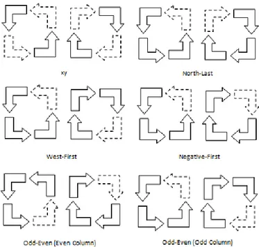
In N-dimensional meshes, deadlock-free routing algorithms can be designed using Turn-model [1][2][3]. As illustrated in Figure 2-10, in Turn-model based routing algorithms, some turns are restricted and packets are not allowed to make them in a network. Using channel dependency graphs (CDG) and keeping away from circular communications is a method that is helpful in networks with any kind of topology. [17].

In a 2D mesh network, at least two turns should be banned for a deadlock free routing algorithm [3].

Theoretical Background

15

Figure 2-10.Turn model-based routing algorithms for mesh topology NoC

In X-Y routing, if the column of the source and the column of the destination are different, a packet moves along the horizontal axis toward the destination. After that it makes progress to the destination vertically. In Figure 2-11, source node (3,1) is communicating with (1,3). The path which is shown using the vector is allowed for sending data from S to D

Figure 2-11.Allowed path in XY routing algorithm

West-First is another deadlock free routing algorithm for mesh topology NoC. The West-First routing algorithm is more adaptive in compare with X-Y [3][7]. Therefore several paths are available for the packets to make progress toward their destinations. Odd-Even routing algorithm is another partially adaptive routing algorithm and has a higher adaptiveness in compared with the other routing algorithms [3][7]. Packets are not allowed to make an East-North or East-South turn at the nodes that are in an even column of a mesh network. North-West or South-West turn is limited at the nodes that are in an odd column (see Figure 2-10).

Theoretical Background

16

For instance, source node S is sending data to destination node D. Applying Odd-Even routing algorithm, there are three possible paths for sending data from S to D that are depicted in Figure 2-12.

Figure 2-12.Allowed paths in Odd-Even routing algorithm

There are many other deadlock free routing algorithms for mesh topology NoCs [3] [7] [10].

2.8 Evaluation of NoC

2.8.1 Network Simulators

Network simulators are used to model and simulate the behavior of a network and evaluate its performance. Building a hardware prototype for a network is very costly and time consuming. For instance, simulators are used to compare routing algorithms. Noxim and Network Simulator (NS2) are two simulators commonly used by researchers. Different options for modeling NoCs are SystemC, SDL, C/C++, Java etc. The research group in Jönköping University has developed a specific NoC simulator based on source routing [12]. This simulator will be modified and used in this project. We modeled Junction Based NoC using SDL.

2.8.2 Performance Parameters

Some of the most important parameters that are used in evaluating the performance of NoCs are defined in this sub-section briefly. These parameters are discussed in details in next chapters.

Latency

Network latency presents the required time to transfer n bytes of payload from its source to its destination. Latency consists of routing delay, contention delay, channel occupancy and overhead.

Theoretical Background

17

 Routing delay is a function of the distance between a source node and a destination node. It also depends on the routing algorithm that is used.

 A number of bits is required for storing routing information, error detection etc. Channel occupancy depends on these kinds of bits.

 Packets should compete for the shared resources, like channels, in a NoC. There is also some delay due to the waiting time in a switch. Contention delay presents these kinds of delays in a network.

 Packetization at source nodes, de-packetization at destination nodes, synchronization between routers etc. introduces a certain amount of delay in a network, called overhead delay.

Bandwidth

Communication bandwidth is the amount of data that can be moved using a communication link in a unit time period.

Throughput

Throughput is the total number of received packets by the destinations per time unit.

Packet Loss

Packet loss happens when one or more packets do not reach their destination due to the error introduced by the network, the contention for network link or lack of buffer space etc.

Link Load

The offered load is the amount of traffic that is injected by the cores into the network. Network Load is defined as the measure of the real communication traffic in the network, regarding maximum possible traffic. Maximum traffic rate is calculated using the following formula:

Maximum traffic rate = Number of links in the network * Link bandwidth

Other load measures used in NoC are actual traffic rate, average load, traffic load etc. Link load is the amount of data flowing through the link in each direction provided the links are considered bidirectional.

Fault Tolerance

Different kinds of faults can occur in the network and fault tolerance describes the capability of a network and a routing algorithm to still route data in this situation.

In-order Packet Delivery

In-order delivery is the delivery of packets in the same order that they were sent. For example, packets following different paths can cause out-of-order delivery.

Power consumed by the routers and their size are important parameters for evaluating routing algorithms. Small and simple routers are desirable.

Theoretical Background

18

2.8.3 Traffic Types

For evaluating NoC using a simulator, data is transmitted into the network in different ways and performance values are evaluated regarding the traffic. There are several kinds of traffic used for NoC simulation:

Uniform Random

A source selects the destination arbitrarily. It means that each core has an equal chance of being chosen as a destination for receiving data from a core in the network.

Local Traffic

A source selects the destination that is closer to it. The chance to be selected as a destination is reduced exponentially with increase in distance.

Transpose (Used in mesh topology NoCs)

A source that is located at position (x,y) transmits data to the core that is located at position (y,x).

Address Bit Reversal

A source that is presented by address (bm bm-1 ….b1 b0) sends data to the destination represented by address (b0 b1 ….bm-1 bm).

Application Specific

Some systems perform specific tasks and it is possible to have traffic information (communication pairs and volume). Communicating core pairs, communication density and communication bandwidth are determined by the predefined application.

Junction-Based Routing

19

3 Junction-Based Routing

Source routing has an important disadvantage of overhead for storing the path information in header of each packet sent. This disadvantage becomes worse as the size of the network grows. In this chapter we describe a routing technique, called Junction Based Routing (JBR) to remove this disadvantage. The idea of junction based routing is basically derived from the railway networks. Railway networks generally have a few large stations, called junctions which are connected by fast railways. A long distance journeys from a small town to another small town is achieved by first going to the nearest junction close to the source and from there reaching a junction close to the destination. In this chapter concepts and issues of this new routing technique are discussed.

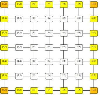
3.1 An Illustration of Junction-Based Routing

Consider the following 7x7 mesh topology NoC that has the diameter of 13 hops (see

Figure 3-1).

Figure 3-1.An illustration of using junctions in a 7x7 mesh topology NoC

The node that is presented using (x,y) is located at

x

y

between nodes that is located at position (x1,y1) and (x2,y2) is calculated using the formula:

Junction-Based Routing

20

The number of routers used from a source node to a destination node is equal to the number of links used plus one. We define hop count as number of routers on the path from a source to the destination.

Hop Count = Distance + 1.

In distributed routing, the header flit stores the address of the destination and for 49 cores, a field of 6 bits is required (2^6=64 cores can be addressed). In source routing the header flit stores the entire path information and a field of 26 bits is used to store the path information (13 hops*two bits for each hop) [4].

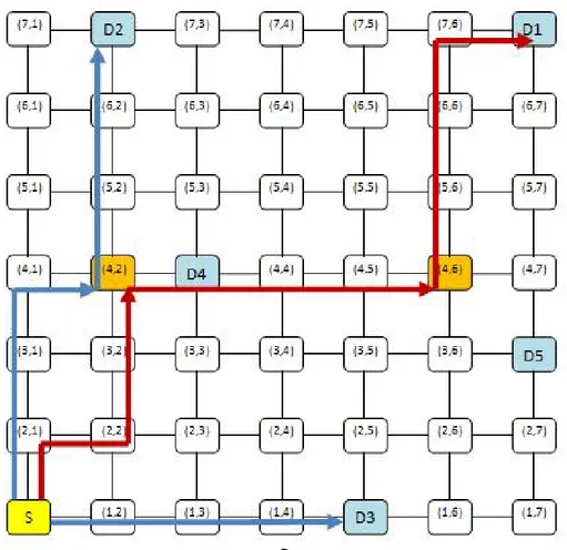
In JBR, the path length is restricted to a constant number of hops, say 6. Therefore, we need a field of only 12 bits to store the path from source to the destination or junction. We give an example to illustrate how JBR will work. Consider that source node (S) is located at position (1,1) and destination node (D1) is located at position (7,7). First junction node (J1) is located at position (4,2) and second junction node (J2) is located at position (4,6). In the next sections, we show that these two junctions are enough to travel in the network with the given hop count limit of six.

S sends the packet to J1 as temporary destination, with the required path information. This junction appends new path information to the packet and forwards it. This new information is necessary to reach the second junction J2. J2 also appends new path information to the packet and forwards it. The information consists of the entire path information from J2 to D1.

To communicate from S to D2 (7,2), J1 is enough and J2 is not used. There is no need to use any junction for sending data to D3 (1,5), because the distance is less than maximum allowed path length (6 hops). A junction can be considered as a normal router for sending packets to next router. This situation happens for communicating between S and D4. Distance between S and D4 is 5 and packet has enough information to reach D4. J1 just forward the packet to the next router.

For sending packets to D5, both of the junctions are used. But length of path increases and becomes 11 hops instead of 9 hops. This issue describes in detail in next sections.

3.2 Analysis of Junction-Based Routing

3.2.1 Packet Format and Path Information

Consider the communicating pair (S,D1) in Figure 3-1. Three types of routing algorithms can be applied i.e. distributed routing algorithm, Junction-Based Routing algorithm (JBR) and source routing. The packet format for each of them is shown in

Figure 3-2. As can be seen the packet header for JBR is so small in compare with

simple source routing, but larger than distributed routing algorithm.

As can be seen, a large distance can be covered by going through intermediate temporary destinations (called Junctions) such that each sub-path (from source to a junction, junction to another junction, and junction to the destination) is smaller than or equal to a maximum hop count.

Junction-Based Routing

21

Figure 3-2.Packet format in distributed routing, source routing and JBR

For the communicating cores with large distance (larger than allowed path length), the source node appends path information from source to a junction. Since the packet entering this junction does not have any information about the output port in its header field, the junction adds the information of path from the junction to the destination or another intermediate junction and forwards it.

The required path information is stored at cores and junctions such that it can be easily used to fill up the required fields in the packet header. The paths can be also computed dynamically. Junctions and resources can also use different mechanism, i.e. resources can use memory tables and junctions can compute the required path using a routing algorithm dynamically. This increases the fault tolerance in the network because junctions can consider the situation of network, like congested links and broken links. But simple source routing has a small fault tolerance. In fact, JBR tries to use the advantages of both source and distributed routing by adding path information in each junction that can consider network situations, like link loads. In distributed routing, each router adds path information for one hop and forwards the packet but in JBR, each junction can add path information for more than one hop. Obviously the architecture of junctions is different from simple routers and delay increases due to replacing path information in each junction. We try some methods to decrease this delay in next chapters.

The idea of JBR is general and will be applicable to all topologies- regular or irregular, but we apply this idea to mesh topology NoC.

Junction-Based Routing

22

3.2.2 Header Overhead in JBR

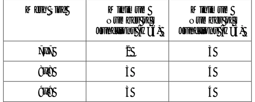
The first purpose in using JBR is to decrease the header overhead. Junctions append the path information using the destination address and packets need to carry the destination address in its header. The following table compares the overhead among distributed routing, source routing and JBR for various network sizes and segment length of 4 hops.

As can be seen from the Table 3-1, the overhead in JBR grows very slowly and therefore it is more scalable. Obviously, there will be a price paid, in terms of routing complications and increased latency in using this technique. In next chapters, we will deal with these important issues.

Table 3-1.The overhead among distributed routing, source routing and JBR for various network sizes Mesh Size Distributed Routing Source Routing JBR

5x5 6 bits 18 bits 8+6 = 14bits

6x6 6 bits 22 bits 14 bits

7x7 6 bits 26 bits 14 bits

8x8 6 bits 30 bits 14 bits

10x10 8 bits 38 bits 16 bits

16x16 8 bits 62bits 16 bits

For a given hop count limit (4), we need 8 bits to store the required path information, two bits for each hop [4]. The destination address needs 6 bits for a 7x7 network. An extra bit in the header is needed to indicate whether the path information is enough to reach the destination or not. In second case, junction will add the path information. In next chapter we describe this completely.

3.3 Challenges in JBR

Source routing is very suitable for small NoC platforms and has many advantages over distributed routing algorithm [4]. Since the packet entering a router has information about the output port in its header field, it simplifies router design and router delay is relatively smaller. Only recently researchers have started considering source routing as a routing candidate in NoCs [4]. Although, the authors in [4] give an analysis of the overhead due to source routing, they have not proposed any solution to reduce/handle the overhead with the size of the network. Some researchers have proposed hierarchical organization of networks and proposed hierarchical routing for large on-chip communication networks [16]. The proposed technique in this paper can be considered as an alternative to their approach.

In JBR, path information for only a few hops is stored in the packet header. With this information, either the packet reaches the destination, or reaches a junction from

Junction-Based Routing

23

where the path information for on-ward path is picked up. If a packet needs to go through a junction (or many junctions) the source just appends path information from source to the first junction. On reaching the junction, the packet picks up path information to reach the destination (or another junction) from this junction. There are many interesting issues related to this approach.

3.3.1 Number and Position of Junctions

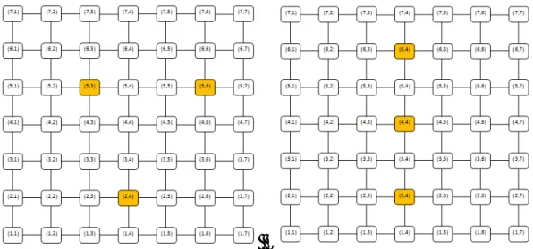
Given the limit on the allowed number of bits available in the header flit for storing path information, a minimum number of junctions will be required to be placed in the network. In a 7x7 network and a given hop count limit of 7, it is easy to see that one junction at the position (4,4) is enough. Figure 3-3 shows this situation.

Figure 3-3 A 7x7 mesh topology NoC with one junction in the middle of network

We developed a MATLAB program that computes the minimum number of junctions and their positions for a given network size and a hop count limit such that the communicating pairs with a hop count larger than a given hop count limit can progress in the network through these junctions.

The pseudo code of the algorithm for calculating the minimum number of junctions and their positions is as following:

N is the network size and H is hop count limit. N and H are input variables for this

function. We generate a graph in which every junction is a node and a pair of junctions has an edge between them if and only if the path length between them is less than the path length limit. This graph must be connected in the sense that there exists a path between any pair of junctions. This condition is necessary for reaching any junction from every other junction.

Junction-Based Routing

24

ALGORITHM Number _Postion_Junctions ( N,H )

{ Num_Junctions := 0; IF (H<2*N-1) { Num_Configurations := 0; WHILE (Num_Configurations == 0) DO { Num_Junctions := Num_Junctions + 1; CALL Jun_Procedure; } } ELSE

PRINT ‘Need No Junction’

}

PROCEDURE Jun_Procedure (Num_Junctions)

{

FOR all possible combinations of Num_Junctions node(s) DO

{

Assume the combination as one of the possible configurations for the junctions;

IF (There is a path from every node to at least one of this (these) junction(s)

with path length less than or equal to H)

THEN

{

Create a graph of these junctions such that there is a link between two nodes of this graph (junctions) iff the path length <= H;

IF (This graph is fully connected) THEN

{

Jun_Configuration:= Jun_Configuration + 1;

Store the selected combination; // As one of the possibilities for placing junctions in the network.

} } }

RETURN Num_Configurations;

Junction-Based Routing

25

3.3.2 A Case Study: Number and Position of Junctions

We use 7x7 mesh topology NoC to illustrate these issues. If path length limit is more than 7 and less than 13 (diameter of the network) then at least one junction is required.

Figure 3-3 shows the position of a junction in the centre of the network, which allows

the use of hop count limit of 7. For hop count limit 6, we require at least two junctions. Figure 3-1 shows the positions of two junctions in the network meeting the requirements listed above.

There are 40 feasible placements of two junction nodes in a 7x7 mesh NoC such that hop count limit of 6 is sufficient.

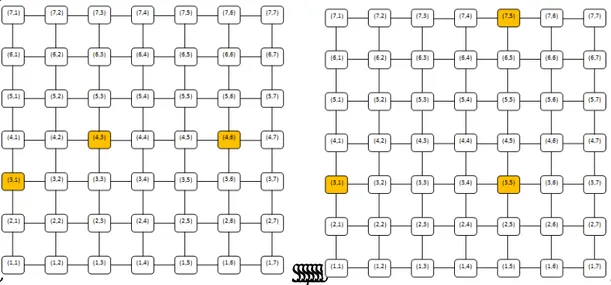
Table 3-2 shows some of different configurations for a 7x7 mesh NoC and a given H

of 5. For instance, one of the possible configurations consists of the nodes that are located at positions (1,3), (3,4) and (6,4).

Table 3-2.Results: Some possible configurations of three junctions which are required for a 7x7 network and a 5 Hop Count Limit

Configuartion No. Positions of Junctions

1 (1,3), (3,4), (6,4) 2 (1,3), (5,3), (4,6) 3 (1,3), (5,3), (5,6) 4 (1,3), (5,3), (5,7) 5 (1,4), (3,4), (6,4) 6 (1,4), (4,4), (6,4) 7 (1,4), (4,4), (7,4) 8 (3,4), (1,5),(6,4) 9 (4,2), (1,5),(5,5)

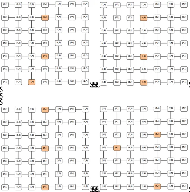
In Figure 3-4, some of the possible configurations for a 7x7 mesh topology NoC and a given H of 5 are depicted.

Junction-Based Routing

26

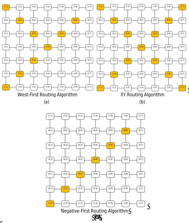
Figure 3-4. Some of different configurations of three junctions which are required for a 7x7 mesh topology NoC and a given H of 5.

Table 3-3 gives the minimum number of junctions required in a 7x7 network for a

given hop count limit. It also gives the number of possible placement of junctions for various cases.

As we see the number of junction(s) is not comparable with the number of all nodes in the network and the number of junctions grows slowly with decreasing the hop count limit.

NJ/NN = (Number of Junction(s))/ (Number of Nodes).

The required number of bits for describing path in a header flit (it is supposed to use worm-hole switching) is calculated as following:

H*2+ (One bit for indicating the completeness of path) + number of bits for addressing the cores.

Junction-Based Routing

27

Table 3-3.Results: Minimum number of junctions and number of possible configurations for a 7x7 network with different Hop Count Limit

Hop Count Limit (H) Number of Junctions (NJ) Number of Configurations NJ/NN Number of Bits

for Path Header

13 0 1 0 33 12 1 45 0.02 31 11 1 37 0.02 29 10 1 25 0.02 27 9 1 13 0.02 25 8 1 1 0.02 23 7 1 1 1/49=0.02 7*2+6+1=21 6 2 40 2/49=0.04 6*2+6+1=19 5 3 80 0.061 17 4 5 691 0.102 15 3 9 1 0.183 13 2 49 1 1 11

Table 3-4 shows the minimum number of junctions that are required for a mesh

topology NoC with different sizes and a given hop count limit (H=6). The number of junctions grows very slowly. For instance, in a 7x7 network (49 cores) the number of junctions is 2 (2/49=0.0408) and in a 10by10 network, the number of junctions is 4 (4/100=0.04).

Table 3-4. Results: Minimum number of junctions for mesh topology NoC with various sizes and a given hop count of 6

Mesh Size Minimum Number of

Junctions (H=6)

7x7 2

8x8 3

9x9 3

Junction-Based Routing

28

Considering each row of Table 3-5, we observe that the number of junctions grows very slowly with the decrease in hop count limit. For instance, the minimum number of junctions is 3 for a 9x9 network and a given H of 6 (3/81=0.037). Number of junctions is 4 for a given H of 5 (4/81=0.049).

Table 3-5. Results: Minimum number of junctions for mesh topology NoC with various sizes and given hop counts of 6 and 5

Mesh Size Minimum

Number of Junctions (H=6) Minimum Number of Junctions (H=5) 7x7 2 3 8x8 3 4 9x9 3 4

Having multiple configuration of junctions for a given path length can be useful for satisfaction of some other criteria like layout uniformity or optimization of performance in the context of application specific communication [10]. As we showed in first section of this chapter, the use of junction based routing can lead to increase in the hop count between some pairs. This average increase in hop count per packet is dependent on the position of junctions as well as on the amount of communications between pairs in the network.

3.4 Increase in Path Length by Using Junctions

In the first section, we observed that path length between S (1,1) and D5(3,7) is increased by going through junctions. In pure source routing, distance between source and destination nodes is 8 but using JBR the distance is 10.

The distance between S (source node) and J1 (first junction) is 4 and the distance between J1 and J2 (second junction) is also 4. The distance between J2 and D4 (destination node) is 2 and therefore, distance between source node and destination node become 10.

Increase in path length is unavoidable while the minimum number of junctions is used. One of the future works in JBR will be to find the minimum number of junctions such that path length does not increase.

3.4.1 Calculating Extra Overhead of Increase in Path Length

Here we describe how to calculate extra overhead of increase in path length in a junction-based network using the following formula:

Extra overhead=





Junction-Based Routing

29 Where,

ij

JD =Distance between node i and node j using Junction based routing

ij

D =Distance between node i and node j using source routing,

ij

V = Communication volume between node i and node j,

M is the total number of nodes in the network and in a 7x7 NoC, M = 49.

For a given junction configuration, the following procedure finds the increase in

average hop count for a set of communications C. Assume the communication ciC

has a volume vi.

We developed a MATLAB function for computing total overhead for all possible configurations for a given Junction-Based mesh network. Input variables are all possible configurations and traffic type or application specific communication matrix.

3.4.2 Results of Computing Extra Overhead Using the Developed Tool

We have computed the average increase in hop count for uniform random traffic and

application specific traffic favoring locality. We make the following

assumptions/choices for our computations.

For modeling a realistic communication traffic we assume that each core communicates with at least one and at most N (Network Size) cores in the network. Communication volume for each pair is a random number in range 1 to 10. Obviously an acknowledgement signal is also taken into account.

PROCEDURE Hop_Count_Increase (C)

{

Total_Overhead := 0;

FOR each communication ci in C DO

{

IF Shortest_path_length > H // H is a given Hop count limit

THEN {

Find the shortest path through junction(s);

Overhead := vi*(L - Shortest_path_length);

// vi is communication volume. For finding shortest path through junctions, we create a graph of junctions and as we know this graph is connected (section 3.3.1). Then a given communicating pair finds the shortest path using finding shortest path in a connected graph that is a common and solved problem.

};

Total_Overhead := Total_Overhead + Overhead; };

Junction-Based Routing

30

For modeling a local traffic we divide the cores into three categories as illustrated in

Figure 3-5. The first category consists of the nodes that are located at the corners of

the network. Second one is the nodes that are located at the boundary of the network and third one includes the other nodes.

The probabilities used for choosing destinations for the nodes that are located at the corners of the network as sources, are as following:

Probability of destination at 1 hop is 15 %, probability of destination at 2 hops is 20 %, probability of destination at 3 hops is 25 % and probability of destination at more than 3 hops is 40 %.

The number of nodes that are located at one hop away from a node that is located at the corners of the network is two. For instance, the source node is located at position (1,1) and it is supposed to choose a destination for this source. Nodes are located at positions (1,2) and (2,1) have 15% chance of being selected as a destination for receiving data from node that is located at position (1,1).

The probabilities used for choosing destinations for the nodes that are located at the boundary of the network as source, are as following:

Probability of destination at 1 hop is 40 %, probability of destination at 2 hops is 30 %, probability of destination at 3 hops is 15 %, and probability of destination at more than 3 hops is 15 %.

The probabilities used for choosing destinations for the other nodes as sources, are as following:

Probability of destination at 1 hop is 30 %, probability of destination at 2 hops is 40 %, probability of destination at 3 hops is15 %, probability of destination at more than 3 hops is 15 %.

Figure 3-5.Three different types of nodes that are categorized depending upon their positions in a 7x7 mesh topology NoC.

Based on our experiments and computations, for a 7x7 mesh NoC with path length limit of 6 hops:

Junction-Based Routing

31

a) For uniform random traffic, the average increase in hop count for different configurations vary between 0.05% to 3%

b) For application specific traffic favoring locality, the average hop count for different configurations vary between 0.01% to 0.09%

It is possible to find the best possible configuration of junctions for a given communication traffic of the application to minimize the increase in extra hop count. Two of the best configurations of junctions in a 7x7 mesh NoC with a given hop count limit of 5 are shown in Figure 3-6. One of the worst configurations is illustrated in Figure 3-7. Figure 3-8 and 3-9 present some of the best configurations and the worst configurations in local traffic respectively.

Figure 3-6.Two of the best configurations of junctions in a 7x7 NoC and a given H of 5 and for a random traffic

Figure 3-7.One of the worst configurations of junctions in a 7x7 NoC and a given H of 5 and for a random traffic

Junction-Based Routing

32

Figure 3-8.Some of the best configurations of junctions in a 7x7 NoC and a given H of 5 and for a local traffic

Figure 3-9.Two of the worst configurations of junctions in a 7x7 NoC and a given H of 5

Junction-Based Routing

33

3.5 Junctions and Deadlock-Free Routing

Presence of junctions makes the network non-homogeneous in the sense that all routers are not identical. A junction router has functionality of a router plus some other functionality. If one is not careful in computing the paths, it can lead to a deadlock.

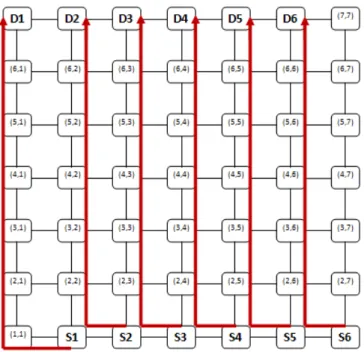
Suppose we want to use negative first routing algorithm for a 7x7 mesh NoC and a given H of 7 (see Figure 3-10). Consider the communicating pair is S (1,7) and D(7,1). Packets have to go through a junction since distance between nodes S1 and D1 is more than 7 hops. The only path between S1 and D1 is shown in the figure. A junction has to be at the position (1,1), because the junction should be close enough to the source and destination nodes and the only possibility is (1,1).

Suppose S is sending data to the node that is located at the position (7,2). Distance between these two nodes is more than 7 hops but the only path between these two nodes does not go through J and J cannot be used for getting the path information. Then another junction is needed for this communicating pair and one junction is not enough.

Figure 3-10.S is sending data to D and it must use node (1,1) as the only possible location for getting the path information from J to D.

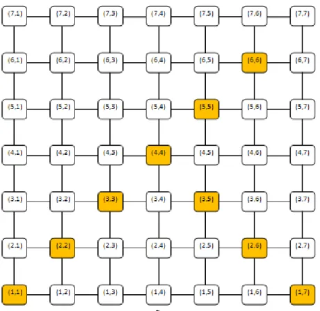
By investigating, we find out that, 6 junctions are needed at least for communication between various nodes using Negative-First routing algorithm. In next chapter, we use a developed MATLAB function that proves that 6 junctions are necessary and sufficient. This is done by exhaustive search of possible solutions. In Figure 3-11 each vector shows the route that is the only possible path for corresponding communicating pair. For instance, for sending packets from (1,7) to (7,6) the only possible route is:

Junction-Based Routing

34 {(1,7) (1,6) (2,6) (3,6) (4,6) (5,6) (7,6)}.

The path length is more than path length limit and using a junction in one of the following nodes is necessary:

{(1,6) (2,6) (3,6) (4,6) (5,6)}.

There are similar situations for the following communicating pairs: (S1,D1), (S2,D2), (S13,D3), (S4,D4) and (S5,D5). The next chapter focuses on deadlock free routing algorithm for a junction based network. Different MATLAB functions are used for finding the minimum number of junctions and their positions for different routing algorithms and also computing paths and finding best paths for different traffic types. Application specific communication is also taken into account.

Figure 3-11. The only possible paths for some of the communicating pairs using Negative-First routing algorithm.