Migration in the
European Union:
Determinants and
Effects of
Enlargement
BACHELOR THESIS WITHIN: Economics NUMBER OF CREDITS: 15 HP
PROGRAMME OF STUDY: International Economics
AUTHOR: Adam Björkman & Oscar Andres
Rodriguez
Bachelor Thesis in Economics
Title: Migration in the European Union: Determinants and the Effects of Enlargements Authors: Oscar Andres Rodriguez & Adam Björkman
Tutor: Mark Bagley and Kristofer Månsson Date: 2017-05-22
Key terms: Migration, Enlargement, The European Union, Labour Market.
Abstract
This paper presents an empirical analysis of the determinants of migration in the European Union with a focus on how enlargements and labour market restrictions affect migration flows. As of 2017, there are five potential candidates that can be part of the next enlargement. Therefore, it is important to analyse if the migration patterns changed with the expansion of the European Union in 2004 and 2007. In the analysis, we estimate the bilateral migration flows from ten origin countries to eleven destination countries in the period 1997-2014 by means of panel least squares. As a theoretical framework, we use the gravity model of migration to analyse the flows while assuming that individuals migrate based on a cost-benefit analysis. The results from the analysis indicate that the migration flows increased significantly in the years that the labour market restrictions were removed. Furthermore, the results from the EU enlargement show a positive effect on migration, although they are not significant across all specifications.
Table of Contents
1.
Introduction ... 1
2.
Background ... 3
3.
Literature Review ... 5
4.
Theoretical Framework ... 7
4.1 Cost-Benefit Analysis ... 74.2 The Gravity Model of Migration ... 8
4.3 Hypothesis and Expected Results ... 9
5.
Data ... 11
5.1 Limitations ... 11
5.2 Variables ... 11
5.3 Descriptive Statistics ... 15
6.
Methodology ... 16
6.1 Empirical Model and Econometric Method ... 16
7.
Empirical Results and Analysis ... 18
8.
Conclusion ... 23
Figures
Figure 1 Migration Flows from 1997-2014 ... 12
Tables
Table 1 Labour Market Restrictions Lifted ... 4 Table 2 Descriptive Statistics ... 14 Table 3 Results from Econometric Model ... 19
Appendix
1. Introduction
The historical expansion of the European Union in 2004 and 2007 brought concerns to the EU151 member states, one of which was the possible large increase in migration from the
adjoining members. The countries that were about to join were in many ways economically weaker than the current members, with a few exceptions. The disparity of income between the EU15 countries and the EU122 countries was a factor that the member states saw as a
potential issue. A fundamental principle of the European Union is the free movement and migration between the member states. Therefore, it was reasonable to believe that the enlargement of the European Union with weaker economies could result in higher levels of migration than desired (Kahanec, Pytlikova, & Zimmermann, 2016).
As of 2017, Albania, the Former Yugoslav Republic of Macedonia, Montenegro, Serbia and Turkey are candidates that are in the process to be a part of the next enlargement of the European Union (European Commission, 2016). If the countries manage to meet the accession criteria and are able to join the European Union, the current member states could once again face a potential large increase in migration due to the income disparities between the old and potential new members. Thus, it is important to review how the membership and labour market restrictions imposed on new members affected migration flows within the new European Union.
In this paper, we will examine migration flows between EU countries before 2004 and the adjoining countries in 2004 and 2007. The purpose is to analyse the determinants of migration within the European Union, with a focus on how a membership in the EU and labour market restrictions affect migration flows.
The migration flows between the countries in our dataset will be analysed by the use of a panel least squares method. We use annual data on migration flows between each of the adjoining countries and each of the existing EU countries from 1997 to 2014. In order to understand the effects of a membership in the European Union and labour market
1 EU15 countries are: Austria, Belgium, Denmark, Finland, France, Germany, Greece, Ireland, Italy, Luxembourg, Netherlands, Portugal, Spain, Sweden and United Kingdom.
2 EU12 countries are: Bulgaria, Czech Republic, Estonia, Latvia, Lithuania, Hungary, Poland, Slovenia, Slovakia, Romania, Malta and Cyprus.
restrictions, we include year dummies for the year the countries joined and for when the labour market restrictions were lifted. As a theoretical framework, we use a gravity model of migration to analyse the flows and a cost-benefit analysis as groundwork for understanding how and why individuals take the decision to migrate.
The research available on international migration is often based on economic theory regarding a cost-benefit analysis in which the potential migrants base their decision evaluating the factors that incur a cost in the movement and also the benefits from migrating with the information available to them at the specific point in time. As a starting point most migration research base their theory on what John Hicks stated in 1932 as “differences in net economic
advantages, mainly differences in wages, are the main causes of migration” (Borjas, Labor Economics,
2016). Most of this research however, has only been able to evaluate migration flows and its determinants by analysing flows into one specific country, done by (Borjas, 1987). Only few authors such as (Mayda, 2010), (Keuntae & Cohen, 2010) and (Kahanec, Pytlikova, & Zimmermann, 2016) have managed to investigate the determinants of migration flows at the international level. This is perhaps due to the constraint of unavailable cross-country data. (Mayda, 2010) Kahanec, Pytlikova and Zimmermann (2016) are one of the few authors that also examine the effect of a membership in the European Union and labour market restrictions on migration flows.
This paper will further contribute to the research regarding the determinants for international migration by investigating the flows within one of the largest single markets in the world. Furthermore, Kahanec et al. (2016) are constrained by the limited time period range after the enlargement since their data only covers migration flows until the year 2010, at this time there were still countries that had restrictions to their labour market. We have managed to collect data that allows us to examine the migration flows between the EU15 and adjoining countries from 1997 to 2014. Hence, we are able to further evaluate the impact of the enlargement and the labour market restrictions on the decision to migrate.
2. Background
Prior to the EU enlargement, only 15 countries were part of the European Union. In April 2003, the current and future member states of the European Union signed a treaty of accession that would result in ten new countries joining the EU in the upcoming year. In 2007, the European Union would further expand to include Romania and Bulgaria and finally in 2013, Croatia became a part of the union. This results in a total of 107.9 million people being granted freedom of movement to the old member states (Kahanec, Pytlikova, & Zimmermann, 2016).
According to the Directive 2004/38/EC of the European Parliament and of the Council, the citizens of the member states have the right to relocate and live in any country belonging to the European Union under the assumption that the individuals are capable of providing for themselves. This is also known as the free movement of labour which is one of the fundamentals for the European Union, as well as the free movement of capital, goods and services (Union, 2004). The directive was a concern for the EU15 countries since it could result in large flows of migrants coming from the new member states. A potential concern could be the challenge of integrating a large number of migrants into labour markets and the society (Meardi, 2012).
The different economic characteristics of the joining countries, one of which were the high income disparities between the EU15 and the EU12 countries, was a potential reason behind the increase in migration. An indicator of the income differences was the GDP per capita PPP which was on average above that of the affiliating countries. In addition, the unemployment levels from the new members were higher than the EU average. Hence, the incentives to migrate should increase when the future earnings are expected to be higher (Alvarez-Plata, Brucker, & Siliverstovs, 2003).
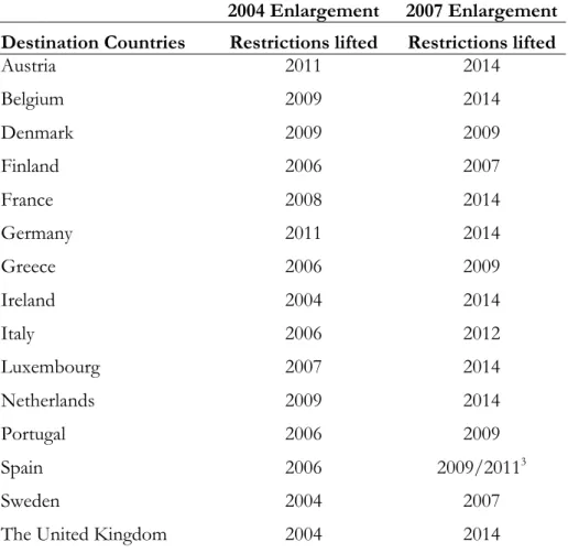
As a response to the potential issue of increased migration, the treaty of accession gave the EU15 countries permission to implement restrictions to their labour markets for the new member states. These restrictions made it possible for the EU15 to delay full access to their labour markets for the citizens of the affiliating countries. The restrictions could be in place for two years, after which a revision had to be made where the state had to provide evidence that their labour market would be negatively affected by the flows of migrants from the
joining states. The EU15 countries could keep the restrictions for a maximum of seven years, although most of the countries chose to remove it early (Kahanec, Pytlikova, & Zimmermann, 2016).
The only three countries who did not choose to implement restrictions in the first enlargement were Sweden, The United Kingdom and Ireland. The majority of countries decided to remove the restrictions before seven years with a few exceptions such as Austria and Germany. Eventually, in 2011, all citizens could have the right to free movement and employment among all member states. This also meant access to social benefits from their new employment. It is important to mention that despite the possibility to restrict access to the labour markets, the self-employed were allowed to immediately migrate and establish themselves in the old member states (Kahanec, Pytlikova, & Zimmermann, 2016).
Table 1: Labour Market Restrictions Lifted.
2004 Enlargement 2007 Enlargement Destination Countries Restrictions lifted Restrictions lifted
Austria Belgium 2011 2009 2014 2014 Denmark 2009 2009 Finland 2006 2007 France 2008 2014 Germany Greece Ireland 2011 2006 2004 2014 2009 2014 Italy 2006 2012 Luxembourg 2007 2014 Netherlands Portugal 2009 2006 2014 2009 Spain 2006 2009/20113 Sweden 2004 2007
The United Kingdom 2004 2014
Source: (Kahanec, Pytlikova, & Zimmermann, 2016)
3. Literature Review
There are numerous studies conducted in respect of the determinants of migrations flows across and within countries. Therefore, it is important to review the most recent and relevant studies that are closely related to the research that is presented in this paper.
Mayda (2010) is one of the most influential authors frequently cited in the international migration literature. Her research is focused on the determinants of international migration and is based on a Cobb-Douglas utility function where an individual takes the decision to migrate if the utility of moving is greater than the utility of staying in the origin country (Mayda, 2010).
For the analysis she combines economic, demographic and cultural variables, as well as controlling for migration policies to reflect the changes in the emigration rate. The chosen explanatory variables are closely related to the gravity model of trade although she expands her model specification by including variables such as share of young population, years of schooling, relative inequality between the countries and the unemployment rate in both origin and destination countries. The data used ranges from 1980 to 1995 and takes into account 79 origin countries’ migration flows to 14 OECD countries.
Mayda’s results are consistent with migration theory, thus she finds that higher income in destination countries, significantly increases the emigration rates. As for geographic distance, she finds that it is negative and significant in all of the different model specifications ran in her study. The only variable that is inconclusive with the theory is the income opportunities in the origin country which in some specifications has a positive impact on the emigration rate although always insignificant.
A similar study with a different approach was taken by Keuntae & Cohen (2010) where they analysed the determinants of international migration by only applying demographic variables in their research. As the theoretical framework they used the gravity model with population in origin and destination countries instead of using a proxy for income such as GDP per capita. The data represents 230 origin countries and 17 destination countries from 1950 to 2007.
Keuntae & Cohen (2010) conclude that their results are in line with the predictions of their gravity model, since they found that large populations in both origin and destination countries significantly increases the immigration flows to the destination countries. As for the distance between the countries, their results are similar to (Mayda, 2010) and the theory since it has a negative impact on the decision to migrate (Keuntae & Cohen, 2010).
Kahanec et al. (2016) provide a recent study that examines the effect of the enlargement of the European Union on migration flows between the EU15 countries and affiliating countries in 2004 and 2007. They focus on the enlargement effect and the labour market openings by the use of dummy variables in the corresponding years and include the usual economic and demographic variables only as control variables. They include data from 1995 to 2010 with 22 destination countries and 10 origin countries. The seven non-EU members are included as destination countries in order to compare the migration flows from the new members to the EU15 with migration flows to the non-EU countries. Thus, they apply a difference-in-difference approach to their analysis.
The economic and demographic variables present the expected impact on migration flows according to theory. The dummies that present EU entry and labour market openings have a positive and significant effect on the migration rate, although the EU entry variable has a larger impact. Hence, the authors conclude that a membership in the EU as well as access to the labour markets is an important determinant in the decision to migrate (Kahanec, Pytlikova, & Zimmermann, 2016).
The previous papers have presented their contribution to the economic migration literature by relying on gravity models which each of the authors modify by the inclusion of possible cultural, demographic or political variables to better explain the migrating decision. A relevant implication to their studies is the unavailability of data at the time of their research. The most comparable research to our topic is that of Kahanec, Pytlikova & Zimmermann (2016) in the sense that they focus primarily on the EU enlargement. It is necessary to mention that although their results are as expected, the data used is constrained due to the fact that two major destinations did not lift their restrictions until 2011. The possibility of studying the determinants and impact of the enlargement on migration flows with new and more reliable data was one of the motivations to undertake the following research.
4. Theoretical Framework
4.1 Cost-Benefit Analysis
The cost-benefit analysis is one of the most fundamental theories used to describe the decision-making process of migrating. The first decision an individual takes, is whether to migrate or not. This is done by weighing the potential benefits and potential costs of moving to a new destination. The potential economic benefit can be described by differences in income opportunities between the destination and origin country. Potential costs include all transportation and relocation costs that are related to the migration process. A rational individual would only migrate if the benefits exceed the costs (Boeri & van Ours, 2013). According to Boeri & van Ours (2013) the decision to migrate can be expressed by:
"#$ = &' ( − &ℎ(() (1 + /)0 1 023 − 40 (1) where NPV is the net present value of migrating which is equal to the sum of all future earnings4 in the destination country (Wf) minus the future earnings in the origin country
(Wh) both discounted by the interest rate. The C0 denotes all costs incurred at the moment of migrating. If the net present value of migrating is positive, then the individual most likely takes the decision to move.
In general, an individual will migrate when:
The differences in the earnings between the destination and origin country are large. The migration costs are low.
The period of benefiting from the earnings differential is longer.
The third proposition implies that it is more beneficial for young people to migrate since they can expect a longer working life. In addition to the tangible benefits and costs presented in the description above, there are numerous intangible benefits and costs that are difficult
to measure. An example of such a cost is the psychological cost of leaving relatives and friends behind (Boeri & van Ours, 2013).
The cost-benefit analysis is useful for understanding the economic intuition behind the decision to migrate for individuals. The analysis focuses on the micro level and varies between individuals as each have different financial situations, costs and preferences. To account for migration flows at the macro level, the gravity model of migration is better suited as it also considers the economic benefits and costs of migrating, but it does so for aggregate individuals within each country. Thus, the gravity model can better represent the patterns of migration by aggregating the decision to migrate taken by thousands of individuals (Kuby, Harner, & Gober, 2004).
4.2 The Gravity Model of Migration
The most recognized gravity model in economics is the one dealing with international trade. According to this model, the trade between two countries can be explained by the product of each country’s GDP or population with the distance between the two as a negative factor. An extension of this framework is the gravity model of migration that is often used to explain migration flows. Both models are based on Newton’s law of gravity, where the attraction between two countries is represented by the mass and the distance. The mass, in terms of economics, is the country’s GDP. The basic representation can be expressed as:
677/8 = 'GDPi ∗ GDPj DISTij
(2) The intuition behind the model is that a higher GDP per capita in the destination country j attracts migrants by the opportunities of earning higher incomes. The distance between country i and country j represents the cost of migration where a larger distance is expected to decrease the migration flows between two countries (Bodvarsson & Van den Berg, 2009). The gravity model for migration has been modified accordingly to include more variables that are relevant in explaining the migration flows. An example of an augmented model is that of (Greenwood, 1997) which can be expressed as
ln 677/8 = b0 + b1 ln D/8 + b2 ln #F#/ + b3 ln POPj + b4 ln J/ + b5 ln J8 + eij (3)
IMMij denotes the migration rate between the origin country i and the destination country j. Dij measures the distance between the two countries while Popi and Popj respectively
represents the population in the origin and destination country. Yi and Yj are the GDP per capita in the source and destination country. The error term e is catching the variation of all the variables that are not explicitly included in the model.
Greenwood’s gravity model specification expects the coefficients of population in origin and destination countries to be positive. This is based on the idea that, all else equal, an origin country with a large population will most likely have more people migrating from it. Also, the larger is the population in the destination country, the more labour market opportunities should be available to migrants. Based on the gravity model theory stated above, the coefficients for both GDP per capita in origin and destination country should be positive and the coefficient for distance is expected to be negative (Bodvarsson & Van den Berg, 2009).
4.3 Hypothesis and Expected Results
Based on the theoretical framework and background section, three hypotheses are formulated in order to investigate the effect of the EU enlargement on migration flows and the determinants of migration within the European Union.
H1: The opportunity of earning a higher income abroad is a significant and positive factor
for migration in the European Union.
Both the gravity model and cost-benefit analysis anticipate that the GDP per capita in the destination country, which can be seen as a proxy for income, has a positive and significant influence on the decision to migrate. A large GDP per capita in the destination country implies higher income opportunities and therefore we expect this variable to be positive and significant.
H2: The enlargement of the European Union caused a significant increase in the migration
The second hypothesis tests whether the concerns about increased migration at the time of the enlargement were legitimate. The enlargement of the EU represents open migration policies even with restrictions imposed, therefore we expect migration flows to have increased even with labour market restrictions.
H3: The removal of the labour market restrictions resulted in a significant increase in the
migration flows.
The cost-benefit analysis suggests that the migration decision is based on the potential benefits. The labour market restrictions restrained migrants from accessing the labour market and obtaining the potential benefits. Thus, we expect the change in migration flows to be higher when restrictions were removed.
5. Data
5.1 Limitations
A recurring issue in previous studies about migration flows is the limited data available. For most of the countries in the European Union the data is well-developed. The OECD, Eurostat and National Statistics Agencies are gathering data of the migration flows as well as the origin of the migrants.
However, for some countries much of the data is still missing. Ireland, Belgium, Greece and Portugal are countries that for different reasons do not have data in regards to the origin of the migrants. As a result, these countries had to be excluded from the empirical analysis. Therefore, the destination countries will be referred to as the EU11 from now on.
In the analysis, Cyprus and Malta will also be excluded from the origin countries as the treaty of accession did not allow any of the EU15 countries to impose restrictions on the free movement or access to the labour markets. Thus, they will not account for the effect of the lifting of labour restrictions. Another drawback from including these two countries is that the data presents many zero flows and missing values that could bias the results. From now and onwards the acceding countries from 2004 will be referred to as the EU+8 countries. Romania and Bulgaria which joined in 2007 will be denoted as the EU+2 (Kahanec, Pytlikova, & Zimmermann, 2016).
5.2 Variables Dependent Variable
The dependent variable that will be used is the migration flows from the old to the new member states, measured in the amount of persons migrating from an origin country to a destination country for every year. Most of the data was obtained from the International Migration Statistics (IMS) database for the OECD countries and only includes legal migration which is based on population registers, residence and work permits (Organisation for Economic Co-operation and Development, 2017).
The data for France and the United Kingdom reported by the IMS is incomplete and suffers from a vast amount of missing values. The reason for the missing data from the UK is that they do not have a population register. Instead, estimates were collected from the Office for National Statistics (Office for National Statistics, 2016). In order to validate if the estimates were reliable, they were compared to the few values reported by the IMS. The source for the data collected from France is from Institut National D’études Démographiques (INED). It includes legal migration based on residence permits from the years 1997-2008 (Institut National D'études Démographiques, 2017).
The graphs below show the migrations flows from all of the origin countries to each of the destination countries over a time period of 18 years from 1997 to 2014. The light blue mark in each of the graphs stands for the year of the first European Union enlargement and the dark blue mark denotes the year of the next enlargement where Romania and Bulgaria became a part of the union. The year that each of the destination countries lifted their restrictions to the labour market for countries adjoining in 2004 is represented by the red mark.5
In the graphs, one can observe that there is an increase in the migration flows the year of both enlargements as well as the year that labour market restrictions were removed for the different countries. Furthermore, in 2008 the financial crisis affected the migration flows and for some countries it temporarily declined. The extent of the impact from the financial crisis is dependent on how severe each country was affected.
5 Sweden and the United Kingdom do not have a red mark since they did not impose any labour market restrictions. Luxembourg and Netherlands removed their restrictions in 2007, the same year as the second EU enlargement, hence they do not have a dark blue mark.
Figure 1: Migrations flows from 1997-2014. 0 20000 40000 60000 80000 1997 1999 2001 2003 2005 2007 2009 2011 2013
Austria
0 5000 10000 15000 1997 1999 2001 2003 2005 2007 2009 2011 2013Denmark
0 5000 10000 1997 1999 2001 2003 2005 2007 2009 2011 2013Finland
0 20000 40000 60000 1997 1999 2001 2003 2005 2007 2009 2011 2013France
0 200000 400000 600000 1997 1999 2001 2003 2005 2007 2009 2011 2013Germany
0 100000 200000 300000 400000 1997 1999 2001 2003 2005 2007 2009 2011 2013Italy
0 1000 2000 3000 1997 1999 2001 2003 2005 2007 2009 2011 2013Luxembourg
0 20000 40000 60000 1997 1999 2001 2003 2005 2007 2009 2011 2013Netherlands
0 100000 200000 300000 1997 1999 2001 2003 2005 2007 2009 2011 2013Spain
0 5000 10000 15000 1997 1999 2001 2003 2005 2007 2009 2011 2013Sweden
0 50000 100000 150000 1997 1999 2001 2003 2005 2007 2009 2011 2013The United Kingdom
Independent Variables
GDP per capita PPP
The variable was collected for both origin and destination countries from the World Bank Database (2017). It is measured in international dollars using purchasing power parity rates, as stated by the World Bank “An international dollar has the same purchasing power over GDP as the
U.S. dollar has in the United States” (The World Bank, 2017). It will be used as a proxy for wages
in the different member states as has been used in previous research by Kahanec, Pytlikova & Zimmermann (2016). Both GDP per capita in origin and destination countries should have a positive effect on migration, although a higher GDP in the destination country should create larger incentives to migrate (Bodvarsson & Van den Berg, 2009).
Population
The source of the data gathered for population in both origin and destination countries is the World Bank Database (2017). It measures total population in each country by accounting for all the residents living in the country regardless of their legal status. These values are mid-year estimates (The World Bank, 2017). As the theory suggests, it is expected that larger populations have a positive and higher impact on migration flows (Bodvarsson & Van den Berg, 2009).
Distance
This variable is collected from the Centre d’Etudes Prospectives et d’Informations Internationales (CEPII) and is calculated as the distance in kilometres between the capital in the origin country and the capital in the destination country (Mayer & Zignago, 2011). The distance is a fundamental part of the gravity model and in the cost-benefit analysis. A shorter distance between countries encourages migration since the cost of moving is lower and individuals tend to have more information about countries that are close to their home country. Therefore, distance should have a negative effect on the decision to migrate (Keuntae & Cohen, 2010).
EU Enlargement dummy
A dummy variable is included to see how a membership in the European Union affects the decision to migrate. The dummy takes on the value of 1 the year the EU+8 and EU+2 countries became a part of the European Union and 0 otherwise.
Labour Market Opening dummy
To find the impact of the labour market restrictions, there is a dummy included that is representing the year the different destination countries chose to lift the restrictions on labour participation for citizens of the adjoining states. Hence, the year an EU11 country removed the restriction the dummy variable takes the value of 1.
Financial Crisis dummy
To control for the effect that the financial crisis in 2008 could have on the migration flows, a dummy is introduced into the econometric model. The dummy takes on the value of 1 for the years each destination country had a declining or stagnating GDP.
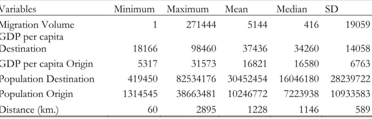
5.3 Descriptive Statistics
The migration volumes between origin countries and destination countries vary substantially. In 1997, 1999 and 2001 there was 1 individual each year that migrated from Slovenia to Finland. Both Slovenia and Finland stand out with a low amount of emigration and immigration in the dataset for all years. The largest migration volume reported in the dataset was in 2007 when 271,444 people migrated from Romania to Italy, which also explains the spike for Italy in Figure 1.From Table 2, it is also possible to conclude that the average GDP per capita in the origin countries is less than half of the average GDP per capita in the destination countries.
Table 2: Descriptive Statistics
Variables Minimum Maximum Mean Median SD
Migration Volume 1 271444 5144 416 19059
GDP per capita
Destination 18166 98460 37436 34260 14058
GDP per capita Origin 5317 31573 16821 16580 6763
Population Destination 419450 82534176 30452454 16046180 28239722 Population Origin 1314545 38663481 10246772 7223938 10933583
Distance (km.) 60 2895 1228 1146 589
N=1880
6. Methodology
6.1 Empirical Model and Econometric Method
The analysis will follow the theoretical framework discussed above and also builds on several aspects from the previous research. The empirical model that will be used is the following:
!" (%&'()*&+" ,+!-./) =b0 + b1 !"(5+6-!)*&+" 7/8*&")*&+"(* − 1)) + b2 !"(5+6-!)*&+" ;(&'&"(* − 1)) + b3 !"(=75 6/( >)6&*) ?/8*&")*&+"(@ − 1)) + b4 !"(=75 6/( >)6&*) +(&'&"(@ − 1)) + b5 !"(7&8*)"C/) + b6(EF E"!)('/./"*) +
b7(H)I+-( J/8*(&C*&+"8) + b8 (L&")"C&)! >(&8&8) + e&M
(4)
The model above will be used to examine the migration flows between a total of 21 countries with a period ranging from 1997 to 2014 estimated by panel least squares with year fixed effects and destination country dummy variables. Since the gravity model includes distance which is time invariant, cross section fixed effects could not be applied. A Hausman test was conducted in order to decide between using a fixed effects model for the years as opposed to a random effects model with cross sections fixed that can estimate the effect of a time invariant variable such as distance. The results of the Hausman6 test suggests that a random
effects model is not suitable.
Although, an issue in the analysis is possibly obtaining biased estimates due to unobserved heterogeneity between the countries in the dataset. To solve for this, dummy variables are included for the different destination countries, instead of cross-sections fixed, to control for unobserved and time-invariant characteristics. This is a common procedure used in previous research and by using least square dummy variables it is possible to estimate distance as well (Mayda, 2010), (Kahanec, Pytlikova, & Zimmermann, 2016).
In the empirical model the dependent variable will be logged as well as the population, GDP per capita and distance. The variables are logged to get rid of skewness in the dataset resulting in a non-normal distribution as can be seen from the histograms in appendix section 3. When the variables are logged, the distribution becomes bell shaped and with a large sample size (n=1779) non-normality should not be an issue. (Gujarati & Porter, 2009)
Furthermore, there are reasons to believe that the migration flows can also have an effect on both GDP per capita and population (Mayda, 2010). Therefore the control variables are lagged one year to resolve the potential issue of endogeneity. By lagging these independent variables, we can be certain that migration flows cannot have an impact on previous values of the GDP per capita or population.
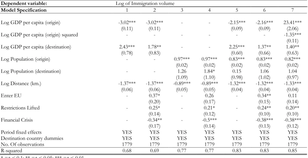
7. Empirical Results and Analysis
Table 3 presents the results from the chosen econometric model. The estimates are overall consistent with the theoretical framework for international migration, with a few exceptions. According to equation (4) the main variables within the gravity model are population and GDP per capita in both the origin and the destination country. The econometric results contain seven specifications to revise the robustness of the estimates. In the first four specifications, the GDP per capita and population are separated and ran both with and without the dummy variables. This is done to check that the estimates are consistent and do not vary across specifications. The GDP per capita and population are introduced together in specifications (5), (6) and (7), where specification (6) and (7) are the full specifications with all control and dummy variables included. Thus, specification (6) and (7) will be used for interpretation.
In specification (7) a quadratic term for the GDP per capita in the origin country is introduced. The results from the first six specifications for the GDP per capita in the origin country contradicts the theoretical framework since the Gravity model suggests that the GDP per capita in the origin country should have a positive effect on migration. A possible explanation for the contradicting results could be that the relationship between migration and the GDP per capita in the origin country follows an inverted U-shaped curve7 (Mayda,
2010).
To test if this variable follows an inverted U-shaped curve, specification (5) is replicated and extended by adding the GDP per capita in the origin both as a linear and a quadratic term. From the output presented in the appendix section 2, it can be seen that the result for the linear term is positive and for the quadratic term is negative, this confirms that the dataset for GDP per capita in the origin country does follow an inverted U-shaped curve. Therefore, the quadratic term is introduced in specification (7).
The most important variables for the purpose of this paper are the enlargement of the European Union- and Restrictions Lifted-dummy, which show the effect of a membership
in the European Union and the restrictions to the labour market on the migration flows. The enlargement-dummy is significant and positive in specification (2) and (6), the former at 10% level of significance and the latter at 5%. Although, in specification (7) it is not significant but remains positive.
The result from specification (6) suggests that in 2004 and 2007, when the origin countries became a part of the European Union, the migration flows from the EU+8 and EU+2 to the EU11-countries increased by 40%8. However, since the variable is insignificant in
specification (4) and (7) the results for the effect of a membership in the European Union on migration is not robust. Thus, the second hypothesis cannot be fully confirmed since it is not possible to determine if there was a significant increase in migration as a result of the enlargements.
A possible explanation to an increase in migration when the countries joined the EU, despite having labour market restrictions, could be the exemption that self-employed individuals could establish themselves immediately in the EU11-countries, as is previously mentioned in the background. Another explanation can be that individuals were allowed to move to the old member states for three months and could extend their stay if they could present evidence that they possessed enough resources to support themselves (Kahanec, Pytlikova, & Zimmermann, 2016). Although, since the results are not always significant, it is difficult to claim that the findings can be applied and generalized outside the sample.
The restrictions lifted dummy is significant and positive in each of the specifications. In specification (7), the variable is significant at the 5% level and shows that the year the countries removed the restrictions to their labour market the migration increased on average by 22%. Hence, this confirms the third hypothesis and from examining the estimates, one can argue that the restrictions implemented were successful. The importance of the labour restrictions get further strengthen since the evidence of a significant increase in migration the year of the enlargement is weaker. Therefore, it is possible to view the restrictions as a mean for delaying migration into the EU11 countries.
Table 3: Results from econometric model.
Panel Least Squares estimates of the determinants of migration flows Dependent variable: Log of Immigration volume
Model Specification 1 2 3 4 5 6 7
Log GDP per capita (origin) -3.02*** -3.02*** - - -2.15*** -2.16*** 23.41***
(0.11) (0.11) (0.09) (0.09) (2.06)
Log GDP per capita (origin) squared - - - -1.35***
(0.11)
Log GDP per capita (destination) 2.43*** 1.78** - - 2.25*** 1.37** 1.40**
(0.78) (0.83) (0.60) (0.66) (0.63)
Log Population (origin) - - 0.97*** 0.97*** 0.83*** 0.83*** 0.82***
(0.02) (0.02) (0.02) (0.02) (0.02)
Log Population (destination) - - 1.26 1.84* 0.15 1.06 1.04
(1.09) (1.10) (0.98) (1.02) (0.97) Log Distance (km.) -1.37*** -1.37*** -0.89*** -0.89*** -1.32*** -1.32*** -1.33*** (0.06) (0.06) (0.05) (0.05) (0.04) (0.04) (0.04) Enter EU - 0.37* - 0.26 - 0.34** 0.11 (0.20) (0.17) (0.15) (0.14) Restrictions Lifted - 0.25* - 0.21* - 0.24** 0.20** (0.14) (0.12) (0.10) (0.10) Financial Crisis - -0.34** - -0.5*** - -0.38*** -0.38*** (0.17) (0.14) (0.13) (0.12)
Period fixed effects YES YES YES YES YES YES YES
Destination country dummies YES YES YES YES YES YES YES
No. Of observations 1779 1779 1779 1779 1779 1779 1779
R-squared 0.68 0.69 0.77 0.77 0.83 0.83 0.85
* =p < 0.1; ** =p < 0.05; *** =p < 0.01
The results for the GDP per capita in destination countries are robust and consistent in every specification where it is included. The estimates support the theory behind the international migration as they are all positive and significant, where an increase in the destination country’s GDP per capita (a proxy for income) increases the migration to the country. This is consistent with the first hypothesis. A higher income in the destination country translates into larger benefits from migrating and according to the cost-benefit theory this will increase the migration. For example, if the GDP per capita increases by 1%, all else equal, the migration volume increases on average by 1.40%. The findings are also supported by the gravity model since GDP per capita in the destination country is one of the attracting forces for migration.
The GDP per capita in the origin country is significant at 1% level of significance and negative across all specifications where it is included only as a linear term, implying that an increase in the GDP per capita in the origin, results in a decrease of the migration from the origin country. As previously mentioned, this contradicts the theoretical framework. In specification (7) where the GDP per capita is included both as a linear and quadratic term, the significance of the estimates show a non-linear relationship which confirms the inverse U-shaped curve.
The intuition behind the U-shaped curve is that when the incomes are low in a country the increase in the GDP per capita will provide the citizens with enough income to account for the cost of migrating and therefore it will have a positive effect. As the country reaches a certain level of income, the incentive of migrating decreases and the GDP per capita will have a negative impact on the migration (Mayda, 2010).
The origin countries in the dataset have high incomes compared to developing countries, therefore it is reasonable to believe that the countries are beyond the level where it shifts from positive to negative. Hence, the origin countries in the dataset are beyond the turning point.
The population in the destination country is only significant in specification (4) at 10% level, in specification (7), the full specification, it is statistically insignificant. A plausible explanation to this, is that the inclusion of GDP per capita in the destination country as well as the dummy variables steal part of the explanation. Since the population variables are only control
variables and the variables of interest are stable and do not change sign across the specifications, the potential multicollinearity should not be a matter of concern.
As for the population in the origin country, it is significant at the 1% level and positive across all specifications, which implies that an origin country with a large population has higher emigration rates. The gravity model anticipates that migration is more likely to occur between countries with large populations. The population in the origin country-variable follows the model’s prediction. The population of the destination country has a positive sign, but it is not significant, and therefore it is not possible to fully confirm the theory.
Distance is a central part of both the gravity model and the cost-benefit analysis and is a representation of the costs of migrating. It is significant and negative in each of the specifications. Hence, the results for the variable are robust and imply that migration flows are smaller between countries that are farther away from each other. The larger the distance between two countries, the higher the costs of transportation and reallocation which increases the up-front cost to migrate. The net present value in the cost-benefit analysis will then be lower and result in less incentives to migrate. The results also correspond to the Gravity Model since it predicts that distance will have a negative effect on migration flows because of the greater costs it represents.
The reason for including the Financial Crisis dummy was to control for the decline in migration to the destination countries which occurred during the years of recession. The estimates are significant in each of the specifications and shows that the years when a country was in a recession the migration decreased. A recession can decrease the probability of finding a job in the destination country and therefore the economic benefit of migrating is lower. Hence, keeping all costs constant the net present value goes down.
8. Conclusion
This paper examines the determinants of migration in the European Union with a focus on how enlargements and the labour market restrictions affects the migration flows. The analysis is done by the use of panel data where it examines the migration flows between 21 countries over a period of 18 years, from 1997 to 2014. The data for the migration flows is gathered from the International Migration Statistics (IMS) of the OECD and National Statistical Agencies.
The results from the research conducted are mostly in line with the theory regarding international migration. Both enlargements of 2004 and 2007 show an increase in the number of migrants into the old member states, although the varying significance of the estimates prevents us from generalizing the results to a context outside the sample. However, the result for the labour market restrictions are robust and shows that the year the restrictions were removed for the different countries, the number of migrants into the EU11 countries increased by 22% on average. This shows that having less restrictive migration policies among the members of the union facilitates the decision to migrate. These results suggest that imposing labour market restrictions on the future potential candidates of Albania, the Former Yugoslav Republic of Macedonia, Montenegro, Serbia and Turkey can help delay or mitigate high migration flows.
The control variables in the analysis suggest that two important determinants for the migration in the European Union are the distance and the GDP per capita in the destination country. The costs of migrating represented by the distance are negative which suggests that individuals tend to move to countries that are close to their country of residence. In regards to the GDP per capita in the destination country, the results show that higher income opportunities abroad attract migrants and results in larger migration flows. If the potential candidates would become members, the increase of migration would most likely occur in countries that are close to the home country and can provide higher income opportunities. Some of the benefits of belonging to the European Union are the free movement of capital, goods and labour between the member states. Although, free labour movement can create concerns among policymakers as the free mobility can result in excess supply of labour. Thus, it is important to have an overview of the migration patterns in order to develop
well-structured and effective integration and migration policies. This paper provides useful insight that can further contribute to the research about international migration and the impact of a membership in the European Union. Hence, it can provide parts of the overview that is needed for policymakers to create a long-term and efficient migration-system.
A limitation in the study is that the data available for migration flows is still incomplete for many countries. As data collecting techniques improve, future researchers can take advantage of more complete data so that the research regarding migration in the European Union continues to develop. In the long-term it will be crucial for the openness of the European Union so the union can continue to promote the free movement of goods, capital and labour among its member states.
The gravity model of migration is useful for understanding and examining migration flows, although it has some limitations. As well as other economic theories, it assumes a closed system where the flows of migration are dependent on two masses that attract each other and the distance between them. Thus, a closed system, such as the gravity model, does not interact with other systems or variables according to its theory. However, in reality economies are open, complex and constantly interacting with other systems (Beinhocker, 2006). As Kuby, Harner and Gober (2013) state in their book Human Geography in Action,
“Human actions are not mechanistically controlled by the size of their origins and destinations or the distances between them”. Therefore it is important to note that, since the European Union is an open
economy, there are other forces that affect migration as well, forces that are not accounted by the gravity model.
9. References
Alvarez-Plata, P., Brucker, H., & Siliverstovs, B. (2003). Potential Migration from Central and Eastern Europe into the EU-15 - An Update. Berlin: DIY Berlin.
Beinhocker, E. D. (2006). The Big Picture. In E. D. Beinhocker, The Origin of Wealth (pp. 68-75). London: Random House.
Bodvarsson, Ö. B., & Van den Berg, H. (2009). The Economics of Immigration Theory and Policy. Berlin: Springer-Verlag.
Boeri, T., & van Ours, J. (2013). The Economics of Imperfect Labor Markets. Princeton, New Jersey: Princeton University Press.
Borjas, G. J. (1987). Self-Selection and the Earnings of Immigrants. The American Economic Review, 531-553.
Borjas, G. J. (2016). Labor Economics (7th Edition ed.). New York: McGraw-Hill Education. European Commission. (2016, December 6). European Neighbourhood Policy And Enlargement
Negotiations. Retrieved from European Commission Website:
https://ec.europa.eu/neighbourhood-enlargement/countries/check-current-status_en Greenwood, M. J. (1997). Internal Migration in Developed Countries. In M. Rosenzweig, & O.
Stark, Handbook of Population and Family Economics (pp. 647-720). Amsterdam: Elsevier.
Gujarati, D. N., & Porter, D. C. (2009). Basic Econometrics. New York: McGraw Hill.
Institut National D'études Démographiques. (2017). Data on Immigration Flows, 1994-2008.
Retrieved from INED Web site:
http://statistiques_flux_immigration.site.ined.fr/en/admissions/
Kahanec, M., Pytlikova, M., & Zimmermann, K. F. (2016). The Free Movement of Workers in an Enlarged European Union: Institutional Underpinnings of Economic Adjustment. In M. Kahanec, & K. F. Zimmermann, Labor Migration, EU Enlargement, and the Great Recession (pp. 1-34). Berlin: Springer-Verlag.
Keuntae, K., & Cohen, J. E. (2010, December). Determinants of International Migration Flows to and from Industrialized Countries: A Panel Data Approach Beyond Gravity. International Migration Review, 44(4), 899-932.
Kuby, M., Harner, J., & Gober, P. (2004). Newton's First Law of Migration: The Gravity Model. In M. Kuby, J. Harner, & P. Gober, Human Geography in Action (pp. 85-106). John Wiley and Sons Inc.
Mayda, A. M. (2010, October). International Migration: A panel data analysis of the determinants of bilateral flows. Journal of Population Economics, 23(4), 1249-1274.
Mayer, T., & Zignago, S. (2011). Notes on CEPII's distances measures: The GeoDist database. CEPII Working Paper 2011-25, 1-12.
Meardi, G. (2012). Social Failures of EU Enlargement. A case of workers voting with their feet. London: Routledge.
Office for National Statistics. (2016, December 1). International Passenger Survey 4.06, country of birth by citizenship. Retrieved from Office for National Statistics Web site: www.ons.gov.uk%2Fpeoplepopulationandcommunity%2Fpopulationandmigration%2Fi nternationalmigration%2Fdatasets%2Finternationalpassengersurvey406countryofbirth
bycitizenship&h=ATN4IFeumtQDBI-_weDIxwaxCEoeRcpdlfhkg2wpbPHhnOeqfdeGHUZezKAnMgTgUzz1_U_TktxYdxnC32 Qa10fawQ_Q_Tvuxu8-K5QWsXO22pzxQ2dMuJ9lOhxuN28BgzghCF3_U-w
Organisation for Economic Co-operation and Development. (2017). International Migration
Database. Retrieved from OECD.Stat:
https://stats.oecd.org/Index.aspx?DataSetCode=MIG
The World Bank. (2017). DataBank World Development Indicators. Retrieved from The World
Bank Web site:
http://databank.worldbank.org/data/reports.aspx?source=2&series=NY.GDP.PCAP.PP .CD&country=
Union, E. (2004). Directive 2004/38/EC of the European Parliament and of the Council. Official Journal of the European Communities, 1-47.
Appendix
1. Inverted U-shaped curve for GDP per capita in origin countries
2. Specification 5 including quadratic term
Panel Least Squares estimates including the quadratic term Dependent variable: Log of Immigration volume
Model Specification 1
Log GDP per capita (origin) 23.75***
(2.05) Log GDP per capita (origin) squared -1.37***
(0.11)
Log GDP per capita (destination) 2.28***
(0.57)
Log Population (origin) 0.82***
(0.02)
Log Population (destination) 0.14
(0.94)
Log distance (km.) -1.33***
(0.04)
Period fixed effects Yes
Destination country dummies Yes
No. Of observations 1779
R-squared 0.85
* = p < 0.1, ** = p < 0.05, *** = p < 0.01
Standard errors in parenthesis
M Ii gr at io n f ro m t he o ri gi n c ou nt ry
3. Distribution with and without logged variables. Dependent and independent variables logged:
0 40 80 120 160 200 240 -3 -2 -1 0 1 2 3
Series: Standardized Residuals Sample 1998 2014 Observations 1767 Mean -2.39e-17 Median -0.044749 Maximum 3.145340 Minimum -2.935881 Std. Dev. 0.848828 Skewness 0.345089 Kurtosis 3.592720 Jarque-Bera 60.93659 Probability 0.000000
Dependent and independent variables not logged:
0 100 200 300 400 500 600 700 800 0 40000 80000 120000 160000 200000 240000
Series: Standardized Residuals Sample 1998 2014 Observations 1767 Mean -3.27e-14 Median -562.5393 Maximum 241467.4 Minimum -26138.59 Std. Dev. 16456.10 Skewness 6.050379 Kurtosis 59.99690 Jarque-Bera 249962.4 Probability 0.000000
4. Dummy variables calculations
Formula for calculating the change of the dependent variable when the dummy takes on the value of 1. [(exp(βi)-1)*100] %
Enter EU dummy = [(exp(0.34)-1)*100] = 40.49%
Restrictions lifted dummy = [(exp(0.20)-1)*100] = 22.14% Financial Crisis dummy = [(exp(-0.38)-1)*100] = -31.61%
5. Hausman Test H0: REM is suitable H1: REM is not suitable
Correlated Random Effects - Hausman Test Equation: Untitled
Test cross-section random effects
Test Summary
Chi-Sq.
Statistic Chi-Sq. d.f. Prob.
Cross-section random 110.728629 8 0.0000
Cross-section random effects test comparisons:
Variable Fixed Random Var(Diff.) Prob.
LOG(GO(-1)) 8.799566 14.330354 0.836883 0.0000 LOG(GO(-1))^2 -0.459795 -0.749770 0.001998 0.0000 LOG(GD(-1)) 2.926161 3.187818 0.026387 0.1072 LOG(POPO(-1)) -2.670229 0.935815 0.562195 0.0000 LOG(POPD(-1)) 0.362172 1.202156 0.382190 0.1742 ENTEREU 0.198463 0.160376 0.000046 0.0000 RESTLIFT 0.238931 0.229647 0.000022 0.0459 FC -0.109058 -0.102226 0.000054 0.3509
Cross-section random effects test equation: Dependent Variable: LOG(MF1)
Method: Panel Least Squares
Sample (adjusted): 1998 2014 Periods included: 17
Cross-sections included: 110
Total panel (unbalanced) observations: 1779
WARNING: estimated coefficient covariance matrix is of reduced rank
Variable Coefficient Std. Error t-Statistic Prob.
C -30.57179 20.58769 -1.484955 0.1377 LOG(GO(-1)) 8.799566 1.689775 5.207538 0.0000 LOG(GO(-1))^2 -0.459795 0.088471 -5.197114 0.0000 LOG(GD(-1)) 2.926161 0.261765 11.17859 0.0000 LOG(POPO(-1)) -2.670229 0.753606 -3.543269 0.0004 LOG(POPD(-1)) 0.362172 0.620886 0.583314 0.5598 LOG(DI) NA NA NA NA ENTEREU 0.198463 0.058501 3.392449 0.0007 RESTLIFT 0.238931 0.063376 3.770080 0.0002 FC -0.109058 0.042642 -2.557525 0.0106 Effects Specification
Cross-section fixed (dummy variables)
R-squared 0.932977 Mean dependent var 6.279864
Adjusted R-squared 0.928256 S.D. dependent var 2.128002 S.E. of regression 0.569988 Akaike info criterion 1.777624 Sum squared resid 539.6361 Schwarz criterion 2.141362 Log likelihood -1463.197 Hannan-Quinn criter. 1.911973 F-statistic 197.6194 Durbin-Watson stat 0.779369 Prob(F-statistic) 0.000000