THESIS
ADAPTING RGB POSE ESTIMATION TO NEW DOMAINS
Submitted by Gururaj Mulay
Department of Computer Science
In partial fulfillment of the requirements For the Degree of Master of Science
Colorado State University Fort Collins, Colorado
Spring 2019
Master’s Committee: Advisor: Bruce Draper
Co-Advisor: J. Ross Beveridge Anthony Maciejewsky
Copyright by Gururaj Mulay 2019 All Rights Reserved
ABSTRACT
ADAPTING RGB POSE ESTIMATION TO NEW DOMAINS
Many multi-modal human computer interaction (HCI) systems interact with users in real-time by estimating the user’s pose. Generally, they estimate human poses using depth sensors such as the Microsoft Kinect. For multi-modal HCI interfaces to gain traction in the real world, however, it would be better for pose estimation to be based on data from RGB cameras, which are more common and less expensive than depth sensors. This has motivated research into pose estimation from RGB images. Convolutional Neural Networks (CNNs) represent the state-of-the-art in this literature, for example [1–5], and [6]. These systems estimate 2D human poses from RGB images. A problem with current CNN-based pose estimators is that they require large amounts of la-beled data for training. If the goal is to train an RGB pose estimator for a new domain, the cost of collecting and more importantly labeling data can be prohibitive. A common solution is to train on publicly available pose data sets, but then the trained system is not tailored to the domain. We propose using RGB+D sensors to collect domain-specific data in the lab, and then training the RGB pose estimator using skeletons automatically extracted from the RGB+D data.
This paper presents a case study of adapting the RMPE pose estimation network [4] to the domain of the DARPA Communicating with Computers (CWC) program [7], as represented by the EGGNOG data set [8]. We chose RMPE because it predicts both joint locations and Part Affinity Fields (PAFs) in real-time. Our adaptation of RMPE trained on automatically-labeled data outperforms the original RMPE on the EGGNOG data set.
ACKNOWLEDGEMENTS
I would like to thank the CSU Department of Computer Science for giving me an opportunity to work on Communicating With Computers Program. I would also like to thank my advisors for their continual support and encouragement in my research. Finally, I would like to thank everyone from the Vision Group for their help and contribution to this thesis. This work was supported by the US Defense Advanced Research Projects Agency (DARPA) and the Army Research Office (ARO) under contract #W911NF-15-1-0459 at Colorado State University.
DEDICATION
TABLE OF CONTENTS
ABSTRACT . . . ii
ACKNOWLEDGEMENTS . . . iii
DEDICATION . . . iv
LIST OF FIGURES . . . vii
Chapter 1 Introduction . . . 1
Chapter 2 Literature Review . . . 6
Chapter 3 Adapting and Retraining RMPE for EGGNOG . . . 9
3.1 Adapting RMPE for EGGNOG . . . 9
3.2 Experimental Methodology . . . 13
3.2.1 EGGNOG data set . . . 14
3.2.2 Inputs and Ground Truth Generation . . . 14
3.2.3 Data Augmentation . . . 17
3.2.4 Network Parameters . . . 17
3.2.5 Evaluation Metrics . . . 17
3.3 Evaluating adapted and retrained RMPE on EGGNOG . . . 18
3.3.1 Goal . . . 18
3.3.2 Methodology . . . 18
3.3.3 Results with the adapted and retrained RMPE . . . 19
Chapter 4 Experiments and Evaluation . . . 22
4.1 Experiments with Spatial Dropout . . . 22
4.1.1 Goal and Hypothesis . . . 22
4.1.2 Methodology . . . 23
4.1.3 Results and Discussion on Experiments with Spatial Dropout . . . 23
4.2 Experiments with Number of Stages in Architecture . . . 25
4.2.1 Goal and Hypothesis . . . 25
4.2.2 Methodology . . . 25
4.2.3 Results and Discussion on Experiments with Number of Stages in Ar-chitecture . . . 26
4.3 Experiments with Number of Training Samples . . . 27
4.3.1 Goal and Hypothesis . . . 27
4.3.2 Methodology . . . 27
4.3.3 Results and Discussion on Experiments with Number of Training Samples 28 4.4 Experiments with Number of Subjects in Training Data . . . 30
4.4.1 Goal and Hypothesis . . . 30
4.4.2 Methodology . . . 30
4.4.3 Results and Discussion on Experiments with Number of Subjects in Training Data . . . 31
Chapter 5 Conclusion and Discussion: . . . 33 Bibliography . . . 35
LIST OF FIGURES
1.1 Goal of Communicating with Computers program: multi-modal communication
be-tween user and agent . . . 2
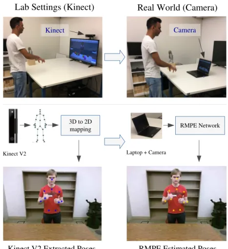
1.2 Lab setup that uses Kinect v2 for pose estimation versus RMPE’s real world applica-tion that uses RGB camera for pose estimaapplica-tion . . . 3
3.1 General architecture of our adapted RMPE: two-staged RMPE . . . 11
3.2 Comparison of Kinect v2 data and input data to our network . . . 15
3.3 Input and Ground Truth . . . 15
3.4 Mean PCK of 10 joints: original RMPE tested on EGGNOG vs. our adapted RMPE trained and tested on EGGNOG . . . 19
3.5 PCK@0.1 and PCK@0.2 for individual joints: original RMPE tested on EGGNOG vs. our adapted RMPE trained and tested on EGGNOG . . . 20
3.6 PCK curves for individual joints: original RMPE tested on EGGNOG versus our RMPE trained and tested on EGGNOG . . . 21
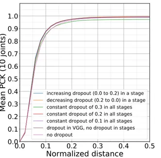
4.1 Mean PCK variations w.r.t. various spatial dropout schemes . . . 24
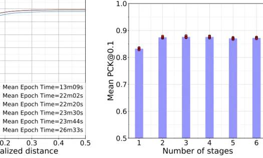
4.2 Mean PCK variations w.r.t. number of stages . . . 26
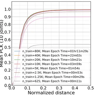
4.3 Mean PCK variations w.r.t. number of training samples . . . 29
Chapter 1
Introduction
Many multi-modal Human Computer Interaction (HCI), activity recognition, and motion cap-ture systems estimate and extract human poses using depth sensors [9]. HCI systems with agents, in particular, interact with users in real-time by estimating the user’s pose. Depth sensors like the Microsoft Kinect have made collection of pose data in laboratories feasible and commonplace. However, automated human pose estimation without the use of depth sensors is a significant goal in the further development of multi-modal human computer interfaces for agents. For this technol-ogy to propagate in the real world, it would be better for pose estimation to be based on data from RGB cameras, which are more common and less expensive than depth sensors. This has motivated an entire branch of literature on skeleton pose estimation from RGB images without using depth sensors. Convolutional Neural Networks (CNNs), in particular, represent the state-of-the-art in this literature [1–6, 10]. Our goal is to estimate human poses using only RGB data with CMU’s RMPE architecture [4] as accurately as what the Microsoft Kinect v2 generates using RGB and depth data.
In particular, this thesis presents a case study on pose estimation using CNNs from either static images or videos without the use of depth sensors. Our task is to adapt the RMPE network to the needs of the DARPA Communicating with Computers (CWC) program [7] as represented by its EGGNOG data set [8]. We chose the RMPE network for its novel architecture that predicts both joint locations and Part Affinity Fields (PAFs) in real-time. Our adapted RMPE network aims to replicate Kinect v2’s skeleton prediction capability in CWC domain without actually using depth sensors. The scientific question being investigated is whether a domain-specific version of RMPE trained on automatically-labeled data will outperform the standard RMPE trained on COCO [11].
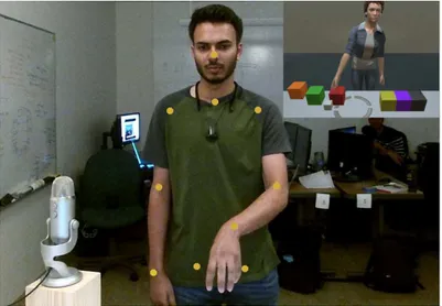
The adapted RMPE generates labeled skeleton poses required by an agent to interact with users in the CWC program. As shown in Figure 1.1, the virtual agent avatar perceives user’s motions through poses predicted by our adapted RMPE. The agent understands user’s gestures by analyzing
predicted joint locations (marked in yellow) and hand poses over time and responds appropriately to the user in the context. In this way, pose estimation facilitates gesture comprehension which in turn helps the system achieve multi-modal communication via gestures and speech. Figure 1.2 shows the adaptation scenario. The left section shows lab settings wherein we extract 2D poses from 3D skeleton estimated by the Kinect v2. Idea is to train adapted RMPE on large-scale Kinect data collected in the lab. This trained network can be used outside the lab to estimate poses from traditional RGB cameras (the right section of Figure 1.2). As compared to the Kinect v2, this setup consisting of a laptop and its build-in camera can be easily deployed in the real world.
Figure 1.1: Goal of Communicating with Computers program: multi-modal communication between user and agent (inset)
Pose estimation using the RMPE architecture has applications in scenarios where a Kinect-like sensors cannot be used for each deployment. One strategy is to collect Kinect data and extract annotated poses to create a training data set. This training data can be used to train an application that predicts poses from RGB images. In this way, deployment of the application does not need Kinect-like sensor. One of the major challenges with current CNN-based pose estimators is that they require large amounts of labeled data with training pairs (RGB images and corresponding 2D poses). If the goal is to train an RGB pose estimator for a new domain, the cost of collecting and more importantly labeling data can be prohibitive. A common solution is to train on publicly
Kinect V2 Extracted Poses RMPE Estimated Poses Kinect V2
3D to 2D
mapping RMPE Network
Laptop + Camera
Lab Settings (Kinect) Real World (Camera)
Kinect Camera
Figure 1.2: Lab setup that uses Kinect v2 for pose estimation versus RMPE’s real world application that uses RGB camera for pose estimation
available pose data sets [11–13], but then the trained system is not tailored to the domain. We propose using RGB+D sensors to collect domain-specific data in the lab, and then training the RGB pose estimator using 2D skeletons automatically extracted from the RGB+D data.
In this thesis, we explore the training and evaluation process of the adapted RMPE pose esti-mation system in the context of the CWC domain. Originally, RMPE was trained and evaluated on COCO [11] and MPII [12] data sets that have different schemes for joint annotation as compared to the EGGNOG data set. Due to this representational shift in joint annotation, the original RMPE model requires modifications in its architecture and parameters prior to retraining on EGGNOG. The modified network is designed to handle the scheme of annotation used in EGGNOG. Specif-ically, we address the question whether RMPE architecture can be used in generalized way for a
new data set other than COCO or MPII on which it was trained. The EGGNOG data set gives an edge in this situation because it has: a) a giant collection of annotated frames and b) a consistent scheme of annotation provided by Kinect v2 that exploits depth channel information. We explore the necessary modifications to the original RMPE architecture and its parameters to get results on EGGNOG that are comparable to using RMPE on EGGNOG. Moreover, we perform studies to reveal effects of different parameters on the performance of the modified network.
Pose estimation techniques like RMPE use CNNs to locate human joints (e.g., head, shoulders, elbows) in RGB images. Usually the goal is to train networks that will perform well across a wide variety of poses, backgrounds, view angles, and imgaging conditions. For instance, RMPE was trained on COCO data set [11] with a diverse set of poses so that it generalizes well across domains. Sometimes, however, applications are more constrained and tightly controlled, in which case it may be possible to train a network that will be more accurate in the context of that application. In this study, we discuss if this sort of specialization achieved by retraining the network benefits the domain of CWC.
One of the most challenging aspects of adapting a pose machine such as RMPE to a new domain is collecting labeled training data. Generally, these networks are trained on manually annotated (hand-labeled) data sets such as the COCO. However the manual labeling is expensive, time-consuming, and prone to mis-labeling and inconsistencies of label definitions. An alternative is to collect training RGB images with co-registered depth images (e.g., with Microsoft Kinect or Intel RealSense sensors) and then use existing 2D-pose-from-depth algorithms to automatically label the joint positions. This approach is not only inexpensive and quick but also makes it easy to collect a large number of labeled training images with a consistent label definition. However, it potentially introduces errors into the training data, since the 2D-pose-from-depth algorithms make mistakes and depth can be noisy. One of the goals of the thesis is to study if this style of training from automatically generated ground truth is feasible.
Our adaptation of RMPE trained on automatically-labeled EGGNOG data outperforms the original RMPE on the EGGNOG data set. The baseline model over which we perform ablation
ex-periments consists of an adapted two-staged RMPE network [4] with both joint and Parts Affinity Fields (PAFs) prediction branches. With this baseline model we study the performance as it varies due to using fewer or more training examples and number of training subjects and also degree of augmentation, fraction of augmented data, degree of regularization with weight decay and with spatial-dropout. We search over these parameters to understand the nature of our modified RMPE architecture. This parameter search is a marginal search along each of these variables while freez-ing the others to some specific value. Our experiments show that it is possible to replicate Kinect v2’s skeleton pose labeling feature with the RMPE architecture trained to predict poses. They also show that RMPE can be used in a generalized fashion to new domains such as EGGNOG. More-over, we demonstrate that retraining RMPE on an automatically annotated pose data set is feasible and the network can be specialized to perform well on the EGGNOG data set. For evaluation we primarily use Percentage of Correct Keypoints (PCK) metric proposed in [14]. On the EGGNOG data set, our baseline model achieves mean PCK@0.1 of 0.879 on a test set 5000 images chosen randomly with only a two-staged network trained on 40K images.
Finally, the road-map of this thesis is as follows. Chapter 2 reviews pose estimation literature addressing architectures and performance of various techniques with a focus on pose machines published by CMU [3, 4]. Chapter 3 introduces our adapted RMPE architecture. It discusses ex-perimental methodology covering brief introduction to the EGGNOG data set, process of inputs and ground truths generation, data augmentation, and network parameters. It then goes over the baseline experiment showing the results of RMPE adaptation. Chapter 4 focuses on various ex-periments on top of the baseline and their evaluation. Purpose of these exex-periments is to perform line-search over parameters to find the best ones in the context of this case study on the EGGNOG data set. Chapter 5 concludes this thesis along with a discussion of possible future avenues for experimentation on pose estimation with the EGGNOG data set.
Chapter 2
Literature Review
Human pose estimation is a critical part of systems such as CWC [7] that study and interact with people. Pose estimation is a challenging problem in computer vision and is an active area of research with its numerous practical applications in HCI [9, 15], motion capture [16], augmented reality [17], etc. For example, Narayana et al. [9] describes a multi-modal interface for the avatar, in which users gesture and/or speak to direct an avatar. Their system exploits body poses (a.k.a. skeletons) estimated by the Microsoft Kinect sensor.
However, since the first application of CNNs to pose estimation problem in DeepPose [1], CNN based methods have consistently established the state-of-the-art for performance. Deep CNNs have propelled the pose estimation algorithms significantly in past few years with various strategies such as iterative refinement of the predictions at each network stage. This progress can be attributed to the ability of these networks to generalize on unseen data facilitated by the availability of large data sets such as MS COCO [11], MPII Human Pose [12], and PoseTrack [13].
Classical methods prior to the advent of CNNs are based on techniques such as pictorial struc-tures [18–21] and graphical models [14, 22]. These methods predict joint locations from hand-crafted features that model interactions between joints. Hand-hand-crafted features limit the generaliza-tion of network on varied human poses in the wild. Recent CNN based methods have regularly outperformed these classical methods by large margins [1–4, 23, 24]. In DeepPose by Toshev et al. [1], the pose estimation problem is formulated as regression to x and y coordinates of joints using a generic CNN. The joint relations were learned instead of designed by hand making the net-work generalizable. Based off this regression concept, Tompson et al. in [25, 26] and Newell et al. in [2] formulated CNNs that regress input images to confidence maps depicting the probabilities of the presence of joints. Moreover, Wei et al. in CPM [3] used a multi-stage CNN for the regres-sion with large receptive fields allowing their network to learn strong spatial dependencies over the successive stages. More recently, Chen et al. in Cascaded Pyramid Network (CPN) [5] address
hard-to-estimate joints with a two-staged architecture consisting of GlobalNet and RefineNet. Xiao et al. in [6] present a simple and effective architecture based on ResNet [27] backbone network with addition of deconvolution layers to predict the confidence maps (heatmaps). These networks are based on the fundamental idea of regressing images to confidence maps.
Recently, Wang et al. released a large-scale video data set called EGGNOG [8] of naturally occurring gestures. This data set contains annotated poses for ~300K frames. EGGNOG is differ-ent from COCO in some aspects. EGGNOG is automatically generated using a Kinect v2 sensor unlike COCO which was manually labeled using Amazon’s Mechanical Turk crowd-sourcing. EGGNOG, therefore, has consistent definitions of where joints should be while COCO has some ‘subjective’ factor due to manual labeling. EGGNOG is a domain-specific data set while COCO is a general-purpose data set with more variance in scales, sizes, backgrounds, poses, etc. of the people in the data set. Similar to COCO, EGGNOG provides avenues to evaluate the CNN based pose estimation methods which is one of the goals of this thesis. It is an open question how well CNN based pose estimation such as RMPE will perform when trained on automatically-extracted skeletons from the EGGNOG. This approach, to our knowledge, of retraining a pose estimation CNN off of a Kinect v2 data set such as EGGNOG to eventually replace the Kinect sensor is not a well-researched topic. It finds applications in HCI systems like CWC where computer interacts with users by understanding 2D human poses.
Methods such as Convolutional Pose Machine (CPM) [3] and RMPE [4] have multi-stage CNNs that formulate pose estimation problem as regression of image to confidence maps depicting joint locations. They use intermediate supervision to address vanishing gradients in deep CNNs. The predictions of these networks are refined over the successive stages as their receptive fields increases in deeper stages. Recent body of work [2–5, 25] show that multi-stage CNNs learn more expressive features and implicit spatial dependencies between joints directly from large-scale data and perform better as compared to classical methods. CPM employs a top-down approach wherein a person detector outputs a detection that is fed to single-person pose estimation network. The runtime of top-down approach is proportional to the number of people in the image. In contrast,
RMPE employs a bottom-up approach wherein a single network detects and estimates joints for all the persons in the image. RMPE uses ‘simultaneous detection and association.’ The network predicts the confidence maps for joint locations followed by associating PAFs that encode part-to-part relations. Cao et al. show that the runtime of RMPE with its bottom-up approach increases relatively slowly with respect to the number of persons in the image. Thus this bottom-up approach is efficient as compared to top-down approach in CPM.
In this thesis, we adopt the common pose estimation formulation which regresses input RGB image to confidence maps. In particular, we concentrate directly on the pose machines published by CMU (CPM and RMPE) [3, 4, 28] that won the COCO 2016 keypoints challenge. We analyze the RMPE architecture on a new large-scale data set - EGGNOG [8] - with the main goal of replicating Kinect v2’s human pose generation capability with a simple RGB camera and CNNs. We contribute by retraining and evaluating RMPE on the EGGNOG data set [29] and by providing an analysis of the RMPE adaptation process to a specific domain.
Chapter 3
Adapting and Retraining RMPE for EGGNOG
Our goal is to determine whether RMPE can be retrained for a specific domain without manu-ally labeling data, and if doing so produces a network that outperforms the standard RMPE trained on a general-purpose data set. This section describes how RMPE is adapted and retrained for the EGGNOG domain. In order to address our goal of estimating Kinect-style 2D poses from RGB images we adapt and retrain RMPE on the EGGNOG data set. The adaptations are necessi-tated primarily due to the differences between COCO on which RMPE was trained originally and EGGNOG on which we retrain RMPE. The differences include factors such as dissimilar schemes of joint annotations and training set characteristics. The adaptations facilitate retraining RMPE on skeleton pose data from EGGNOG that was generated by Kinect v2. We overview the methods and experiments that describe our adapted RMPE along with the results of the experiments. We address the primary question of how an adapted RMPE architecture trained on EGGNOG - having large-scale, domain specific, and potentially noisy Kinect data - performs relative to the RMPE trained on a general-purpose COCO data set. In brief, we aim to illustrate the RMPE adapta-tion process and educate about domain-specific retraining. Secadapta-tion 3.1 below discusses network implementation details covering data set overview, data pre-processing, network parameters, and evaluation metrics. The experiment answering our primary question is called baseline experiment on top of which experiments from chapter 4 are conducted.
3.1
Adapting RMPE for EGGNOG
Prior to discussing the architectural details of our adapted RMPE, we will discuss the charac-teristics of the EGGNOG data set that motivated the modification to RMPE architecture. Ideally, we would retrain RMPE without changing its architecture in any way, to create to perfect apples-to-apples comparison in the Section 3.3. Unfortunately, differences between the COCO and the EGGNOG data sets require small architectural changes. Users in EGGNOG are standing behind
a table; their legs and feet are not visible. We therefore train RMPE to detect the 10 upper body joints (listed in the Section 3.2) that are common to the Microsoft skeleton and the COCO data labels, meaning that our adapted RMPE predicts 11 confidence maps (10 for joints and one for background) and 18 PAF maps corresponding to the joint connectors formed by those 10 joints. In contrast, RMPE predicts 19 confidence maps and 38 PAF maps because its training set (COCO data set) contains 18 annotated joints and corresponding 38 joint connectors. Therefore we change the final convolutional layer at every stage of RMPE to predict the modified number of feature maps i.e., 11 joint confidence maps and 18 PAF maps. Another necessary modification was the addition of spatial dropout layers after convolutional layers to avoid overfitting that was observed when dropout was not introduced. With these modifications, we built a baseline system that exper-iments with our adapted RMPE (shown in Figure 3.1) by retraining it for CWC domain represented by EGGNOG.
Figure 3.1 shows our modified RMPE. The details are similar to those in [4]. Similar to the original RMPE, our network produces a set of 2D confidence maps (Figure 3.3b first row) and 2D Part Affinity Field vectors (PAFs) (Figure 3.3b second row) for an input image of size h × w . Locations of joints in 2D pixel space are then extracted from the predicted 2D confidence maps using simple non-max suppression methods described in RMPE paper [4]. The network outputs J confidence maps - one corresponding to each joint - denoted by S in Figure 3.1. It also outputs C affinity vector maps (PAFs) - one corresponding to each limb formed using pairs from set of J joints - denoted by L in Figure 3.1.
The input RGB images are fed through the VGG feature extractor block at the beginning of the network to generate feature maps F (details of VGG block in appendix). This block has first 10 layers of VGG-19 [30] network. These feature maps (F) are fed as input to both the branches of stage 1. The first stage outputs confidence maps S1 = ρ1
(F) and PAF maps L1 = φ1
(F) where ρ1 andφ1
are the CNNs from branch 1 and 2 of the first stage. The structure of convolutional block for every stage after stage 2 is identical to stage 2 block structure. For each stage after stage 1, the predictions from both the branches of the previous stage and VGG feature maps F are concatenated and fed as input to the next stage such that,
St= ρt(F, St−1, Lt−1), ∀t ≥ 2, (3.1)
Lt= φt(F, St−1, Lt−1), ∀t ≥ 2, (3.2) where, ρt andφt are the CNNs from branch 1 and 2 of stage t. This formulation is similar to what is proposed in [4].
Replicating the loss functions from original RMPE, we useL2 loss function at the end of each stage to enforce intermediate supervision. For each stage, the losses are calculated at the end of each branch between predicted feature maps and ground truth feature maps. Similar to [4], for stage t the losses are calculated as follows,
fSt = J X j=1 kStj − S∗jk 2 2, (3.3) fLt = C X c=1 kLt c− L∗ck 2 2, (3.4)
where S∗j and L∗c are the ground truth confidence maps and PAF maps respectively. We discuss the process to generate ground truth for EGGNOG in the Section 3.2.2. Total loss f of the network is sum of all the losses at each stage and each branch defined by,
f= T X t=1 (ft S+ fLt), (3.5)
where, ftS and ftL are the losses at stage t for the confidence map predictor and PAF predictor branches respectively.
We observed that lesser degree of augmentation of training data helped achieving better perfor-mance as compared to higher degree of augmentation used in original RMPE. The augmentation parameters used in this thesis are discussed in the methodology below. We keep the network learn-ing parameters and weight decay parameters as same as the original RMPE model.
PAFs are beneficial to establish association between body parts (joints) when there are multiple subjects present in input image. In the EGGNOG data set we have only one subject per image frame. However, we concluded experimentally that having a PAF predictor branch in the network boosts the PCK performance even when only one subject is present.
3.2
Experimental Methodology
Retraining RMPE on EGGNOG requires input and ground truth pairs. EGGNOG, being a Kinect data set, provides the data in video format along with 2D pose annotations for each frame in the video. These 2D poses are generated from 3D poses and depth information captured by the Kinect. Before the individual RGB frames can be fed to our network, they need pre-processing to make them compatible with the network architecture. We also augment the data to encourage network to generalize. In order to facilitate network learning for each input we need the ground truths against which we compare the predictions. Ground truths are Gaussian belief maps and they are generated using the methodology in [4]. The following sections introduce the EGGNOG data set, input pre-processing, ground truth generation, and data augmentation. Finally, we review the standard evaluation metrics used for pose estimation models.
3.2.1
EGGNOG data set
The EGGNOG data set [8] has over ~300K RGB image frames distributed among 360 trials and 40 human subjects with the videos spanning over 8 hours. It was recorded using a Microsoft Kinect v2 sensor that outputs poses in 3D. EGGNOG also provides corresponding 2D poses that are extracted from 3D poses using 2D-pose-from-depth algorithm. It provides 25 joints annotated with a scheme provided by Kinect v2. EGGNOG is an upper-body data set Figure 3.2a with only 19 joints from hips and above out of original 25 joints visible in the frames. The experiments conducted in this thesis use only 10 joints which are Head, Spine Shoulder, Left Shoulder, Left Elbow, Left Wrist, Right Shoulder, Right Elbow, Right Wrist, Left Hip, and Right Hip as shown in Figure 3.2b. We divide the EGGNOG data set in training, validation, and testing sets containing 28, 8, and 4 subjects respectively.
3.2.2
Inputs and Ground Truth Generation
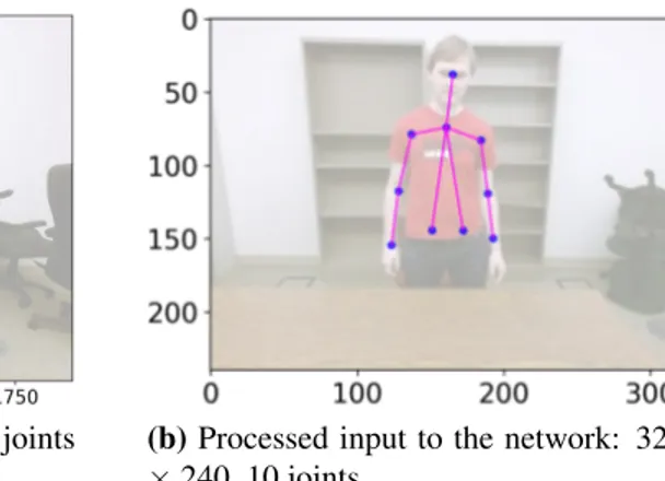
Inputs:Data collected by Kinect v2 has resolution of 1920× 1080 pixels. We extract individual frames from the video data in .avi format yielding image frames of size 1920× 1080 pixels (Figure 3.2a). From this high resolution image, we crop out extraneous patches of width 240 pixels from left and right side of the image based on the observation that the subject in EGGNOG approximately stays in the center the image. Next, we reduce both the dimensions of image by a factor of 4.5 to get an image of size 320× 240 pixels. This lower resolution image (Figure 3.2b) is closer to what original RMPE uses (368× 368) as input and it also allows the network to train faster as compared to high resolution input images.
EGGNOG provides annotations for 19 visible joints. However, some of the joints such as thumb and hand tips are noisy. Therefore, we decided to exclude those joints from our analysis. In order to have one-to-one comparison with original RMPE, we work with only 10 joints that are common between the COCO and EGGNOG data sets. Figure 3.2a shows (in red dots) all 19
joints visible in EGGNOG and Figure 3.2b shows (in blue dots) the only joints that we used during training.
(a) Kinect v2 data: 1920× 1080, 19 upper body joints (b) Processed input to the network: 320 × 240, 10 joints
Figure 3.2: Comparison of Kinect v2 data and input data to our network
Ground Truth:
We use the algorithms specified in the ‘Method’ section of RMPE paper [4] to generate the ground truth confidence maps S∗ and PAF maps L∗.
(a) Input RGB image (320× 240 × 3) (b) Ground truth (40 × 30): first row - confidence maps for left elbow and left wrist; second row - PAF maps (x and y) for joint connector from left elbow to left wrist (left hand since images are flipped horizontally)
The confidence maps are Gaussian in 2D pixel space representing the belief that a joint occurs at specific pixel location. To generate the confidence map for joint j, we use the 2D joint annota-tions (xj ∈ R
2
) from Kinect data after transforming them to a 40× 30 ground truth space. First row of Figure 3.3b shows the confidence maps for right elbow and right wrist overlaid on down-sampled input image. Values in confidence map range from 0 to 1 with 0 meaning no belief and 1 meaning complete belief that a particular joint in present at that pixel. The value of confidence map for joint j at pixel location p∈ R2
is defined by,
S∗j(p) = exp(−α × kp − xjk 2
2), (3.6)
where,α determines the spread of the Gaussian belief map.
The PAF maps are generated for all the joint connectors c from the set of joint connectors C. Consider a joint connector c formed by connecting joint j1 at location xj1 to j2 at location xj2. The value of PAF map for a joint connector c at pixel location p∈ R2
is defined by, L∗c(p) = v if p is on joint connector c. 0 otherwise. (3.7)
Here, v is a unit vector from joint j1to j2defined by,
v= (xj2 − xj1)/kxj2 − xj1k2, (3.8) A point p is considered to be on the joint connector c if it follows
0 ≤ v · (p − xj1) ≤ lc and|v⊥· (p − xj1)| ≤ σl. (3.9)
Here, lc = kxj2− xj1k2is the length of the joint connector from joint j1to j2 andσlis the width of the same connector in pixels.
3.2.3
Data Augmentation
We augment the RGB images by randomly choosing an angle of rotation from [-12°, +12°], scaling factor from [0.8, 1.2], horizontal flipping probability of 0.5, and translation value (in num-ber of pixels) along horizontal and vertical direction from [-40, 40]. While generating the joint confidence maps and PAF maps for EGGNOG, we selectedα = 2.25 and limb width (σl) = 0.75 in equation 3.6 and 3.7 respectively.
3.2.4
Network Parameters
We train our modified network with network parameters identical to what original RMPE used. For our network, the base learning rate is4 × 10−5, the momentum factor for Stochastic Gradient Descent (SGD) optimizer is 0.9, and the weight decay factor is5 × 10−4. For the EGGNOG data set the network converges after approximately 100 epochs as determined by inspecting the network loss graphs on validation set.
3.2.5
Evaluation Metrics
We evaluate our experiments with Percentage of Correct Keypoints (PCK) and Percentage of Correct Keypoints w.r.t. Head Segment (PCKh) metrics. We also report the Area Under the Curve (AUC) for the PCK curves.
For PCK metric, a keypoint is considered to be predicted correctly if its predicted location falls within some normalized distance from its ground truth location. As proposed in [14], the normalized distance is defined using the formula α · max(h, w ), where h and w are respectively the height and width of the tightest bounding box that encloses all the ground truth keypoints of the particular test sample. Multiplier α is varied from 0 to 0.5 to control the normalized distance threshold used to decide correctness of predicted keypoint. We varyα only up to 0.5 because for α > 0.5 the ‘PCK versus Normalized Distance’ plot saturates to PCK ≈ 1.0. As α becomes 1.0, the allowed margin for error increases to approximately 97.36 pixels which is a large margin with respect to the size of the test image (320× 240 pixels).
In PCKh metric the normalized distance is calculated with respect to the length of the head segment of the subject. Head segment in case of the EGGNOG data set is the segment from Head joint to the Spine Shoulder joint. The results sections of all the experiments in this thesis only discuss the PCK metric.
3.3
Evaluating adapted and retrained RMPE on EGGNOG
3.3.1
Goal
The primary goal of this baseline experiment is to demonstrate replication Kinect v2’s skeleton prediction capability by adapting RGB based pose estimation techniques, in particular, the RMPE. This experiment also addresses if retraining RMPE in new domains such as CWC is beneficial in achieving better PCK performance as compared to using off-the-shelf, pre-trained RMPE network. This experiment establishes a baseline PCK score against which we compare results from all the experiments in chapter 4 involving line-search for the best network parameters.
3.3.2
Methodology
The adapted RMPE Network for this experiment consists of a two-staged RMPE network si-multaneously predicting both the joint locations and PAFs as shown in Figure 3.1. Each stage iteratively refines the predicted joint locations. The training set consists of 40000 images evenly distributed among 28 subjects (from 14 trial sessions of EGGNOG) and validation set consists of 4000 images evenly distributed among 8 subjects (from 4 trial sessions of EGGNOG). We reserve 4 subjects for the test set to evaluate all the experiments discussed hereafter. This network pre-dicts location feature maps (confidence maps) for 10 joints listed in the experimental methodology (Section 3.2).
We compare performance of RMPE and our model on a test set of 5000 images chosen ran-domly from the test set of the EGGNOG data set. We use two metrics viz., Percentage of Correct Keypoints at normalized distance of 0.1 (PCK@0.1) and Area Under the Curve (AUC) calculated for the ‘PCK against Normalized Distance’ plot.
3.3.3
Results with the adapted and retrained RMPE
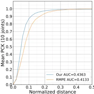
Figure 3.4 shows mean PCK plots for 10 joints on the same test set of 5000 images. The red curve is when the test set is fed through the off-the-shelf RMPE weights while the blue curve is when we modify and retrain the RMPE network specifically for EGGNOG.
In order to emphasize advantages of retraining the RMPE for the specific domain of EGGNOG, we use PCK@0.1 as a metric to compare our results with RMPE’s results. PCK@0.1 corresponds to a normalized distance of approximately 9.74 pixels on this test set with images of size 320× 240. PCK@0.1 for our modified RMPE model is 0.8797, whereas for the original RMPE model it is 0.7009. From the performance of our model, we can conclude that it is possible to replicate Kinect v2’s skeleton prediction capability using the modified RMPE network with almost 87.97% accuracy. Increased PCK@0.1 score suggests that retraining RMPE for our specific domain of the EGGNOG data set helps in reducing the errors in prediction of joint locations. To understand the overall performance with various thresholds of normalized distances, we use the AUC metric. AUC of baseline experiment is 0.4363 while AUC for original RMPE model is 0.4133 which means that our model’s overall performance is better than the overall performance of RMPE on EGGNOG.
0.0
0.1
0.2
0.3
0.4
0.5
Normalized distance
0.0
0.1
0.2
0.3
0.4
0.5
0.6
0.7
0.8
0.9
1.0
Mean PCK (10 joints)
Our AUC=0.4363 RMPE AUC=0.4133Figure 3.4: Mean PCK of 10 joints: original RMPE tested on EGGNOG vs. our adapted RMPE trained and tested on EGGNOG
Head Spine Shld (Neck)
Left ShldLeft ElbowLeft WristRight ShldRight ElbowRight WristLeft HipRight Hip
0.2 0.4 0.6 0.8 1.0 PCK@0.1 RMPE Our (a) PCK@0.1 Head Spine Shld (Neck)
Left ShldLeft ElbowLeft WristRight ShldRight ElbowRight WristLeft HipRight Hip
0.2 0.4 0.6 0.8 1.0 PCK@0.2 RMPE Our (b) PCK@0.2
Figure 3.5: PCK@0.1 and PCK@0.2 for individual joints: original RMPE tested on EGGNOG vs. our adapted RMPE trained and tested on EGGNOG
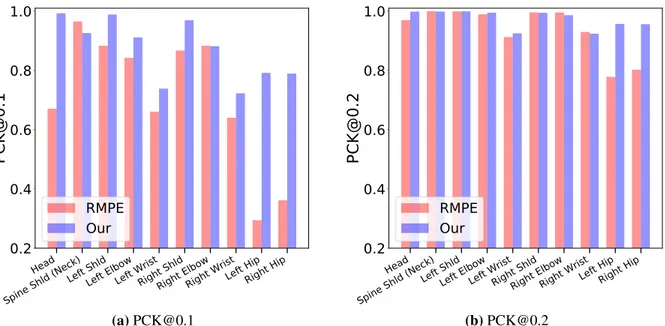
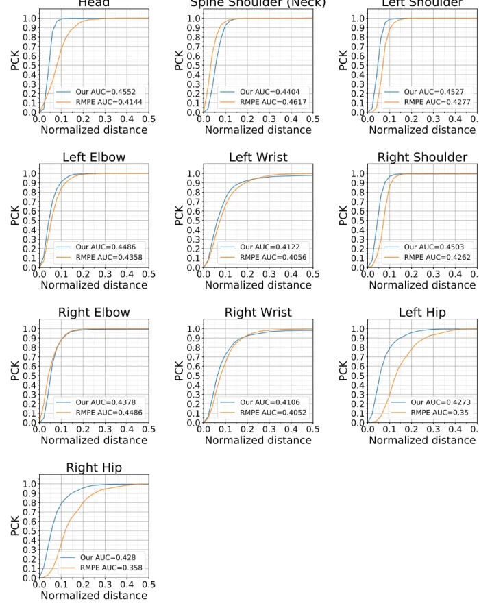
In order to understand how well the prediction of individual joints is working, we analyzed results of our network and the RMPE network for individual joints as shown in Figure 3.5a, Fig-ure 3.5b, and FigFig-ure 3.6. Except for two joints (Spine Shoulder and Right Elbow), our modified model gives better performance for PCK@0.1 as compared to RMPE model. RMPE performance is particularly poor for the hip joints (LHip and RHip). This may be because RMPE was trained with definitions of hip joints defined by COCO and EGGNOG test set has slightly different defini-tions of where the hip joints should be located.
0.0 0.1 0.2 0.3 0.4 0.5 Normalized distance 0.0 0.1 0.2 0.3 0.4 0.5 0.6 0.7 0.8 0.9 1.0 PCK Head Our AUC=0.4552 RMPE AUC=0.4144 0.0 0.1 0.2 0.3 0.4 0.5 Normalized distance 0.0 0.1 0.2 0.3 0.4 0.5 0.6 0.7 0.8 0.9 1.0 PCK
Spine Shoulder (Neck)
Our AUC=0.4404 RMPE AUC=0.4617 0.0 0.1 0.2 0.3 0.4 0.5 Normalized distance 0.0 0.1 0.2 0.3 0.4 0.5 0.6 0.7 0.8 0.9 1.0 PCK Left Shoulder Our AUC=0.4527 RMPE AUC=0.4277 0.0 0.1 0.2 0.3 0.4 0.5 Normalized distance 0.0 0.1 0.2 0.3 0.4 0.5 0.6 0.7 0.8 0.9 1.0 PCK Left Elbow Our AUC=0.4486 RMPE AUC=0.4358 0.0 0.1 0.2 0.3 0.4 0.5 Normalized distance 0.0 0.1 0.2 0.3 0.4 0.5 0.6 0.7 0.8 0.9 1.0 PCK Left Wrist Our AUC=0.4122 RMPE AUC=0.4056 0.0 0.1 0.2 0.3 0.4 0.5 Normalized distance 0.0 0.1 0.2 0.3 0.4 0.5 0.6 0.7 0.8 0.9 1.0 PCK Right Shoulder Our AUC=0.4503 RMPE AUC=0.4262 0.0 0.1 0.2 0.3 0.4 0.5 Normalized distance 0.0 0.1 0.2 0.3 0.4 0.5 0.6 0.7 0.8 0.9 1.0 PCK Right Elbow Our AUC=0.4378 RMPE AUC=0.4486 0.0 0.1 0.2 0.3 0.4 0.5 Normalized distance 0.0 0.1 0.2 0.3 0.4 0.5 0.6 0.7 0.8 0.9 1.0 PCK Right Wrist Our AUC=0.4106 RMPE AUC=0.4052 0.0 0.1 0.2 0.3 0.4 0.5 Normalized distance 0.0 0.1 0.2 0.3 0.4 0.5 0.6 0.7 0.8 0.9 1.0 PCK Left Hip Our AUC=0.4273 RMPE AUC=0.35 0.0 0.1 0.2 0.3 0.4 0.5 Normalized distance 0.0 0.1 0.2 0.3 0.4 0.5 0.6 0.7 0.8 0.9 1.0 PCK Right Hip Our AUC=0.428 RMPE AUC=0.358
Figure 3.6: PCK curves for individual joints: original RMPE tested on EGGNOG versus our RMPE trained and tested on EGGNOG
Chapter 4
Experiments and Evaluation
We showed with the baseline experiment that RMPE can be trained using Kinect data; in fact it outperforms the original at least for the EGGNOG task domain. In this chapter we discuss a set of experiments dealing with network parameters and architecture. These experiments analyze effects of various factors on training and the performance of our modified RMPE network. Our goal is to understand the network retraining process revealing interesting findings on RMPE’s practical application to CWC project represented by the EGGNOG data set. In particular, we show how factors such as spatial dropout, number of RMPE network stages, number of training subjects, number of training samples, data augmentation, etc. affect the performance of our network. This study basically illustrates network parameter search.
In the Section 4.1, we begin with the experiments that study the effects of spatial dropout introduced to address the overfitting issue while retraining RMPE on the EGGNOG data set. The Section 4.2 contains experiments that analyze how number of stages in RMPE architecture affect its performance. The Section 4.3 describes experiments analyzing the effect of number of training samples on the performance of our network. The Section 4.4 contains experiments addressing the question of how many subjects should be included in the training set.
4.1
Experiments with Spatial Dropout
4.1.1
Goal and Hypothesis
One of the changes moving from the original RMPE to our baseline model (described in chapter 3) was the use of spatial dropout techniques to avoid overfitting. We observed that the addition of spatial dropout layers after each convolutional layer reduced the overfitting on the EGGNOG data set. For the baseline experiment we use a constant dropout rate of 0.2 for every spatial dropout layer after the convolutional layers in each stage. We observed that the original RMPE with no dropout
overfits on EGGNOG. The goal was to improve the original RMPE’s performance on EGGNOG by avoiding the overfitting with addition of spatial dropout regularization. In these experiments, we analyze how different dropout strategies affect the network performance.
4.1.2
Methodology
Tompson et al. [26] formulated a new regularization technique of spatial dropout to improve generalization of the trained network while solving pose estimation problem. They found that the standard dropout technique does not prevent overfitting because the pixels within a feature map were still strongly correlated even after dropping out random pixels by setting their activations to zero. To avoid this issue they introduced spatial dropout where activations of entire feature map are randomly set to zero. Similar to their results, we observe improvements in performance of our network with addition of spatial dropout.
In particular, after every convolutional layer we randomly choose a feature map with a certain probability (selected empirically) and set that entire feature map to zero. Meaning all the activation values in that feature map are set to zero. Spatial dropout is significantly effective than normal dropout technique because it drops entire feature map instead of individual values in that feature map. Feature map activations usually exhibit strong spatial correlation. Therefore, with standard dropout technique the network may exploit this spatial correlation to estimate the dropped value. However, spatial dropout avoids this because the entire feature map is dropped and network needs to learn that feature map again. For our network shown in Figure 3.1, we add spatial dropout layers after every convolutional layer with some specific dropout rate.
4.1.3
Results and Discussion on Experiments with Spatial Dropout
Figure 4.1a and Figure 4.1b show the mean PCK scores for five trials of experiments with different versions of spatial dropout. With a dropout rate of 0.0, mean PCK@0.1 score is 0.8462. When spatial dropout with rate of 0.2 is introduced, mean PCK@0.1 increases to 0.8786. If we further increase the dropout rate to 0.3, mean PCK@0.1 drops to 0.8544. We experimented with other variations of the dropout and concluded that for the EGGNOG data set a spatial dropout with
0.0
0.1
0.2
0.3
0.4
0.5
Normalized distance
0.0
0.1
0.2
0.3
0.4
0.5
0.6
0.7
0.8
0.9
1.0
Mean PCK (10 joints)
increasing dropout (0.0 to 0.2) in a stage decreasing dropout (0.2 to 0.0) in a stage constant dropout of 0.3 in all stages constant dropout of 0.2 in all stages constant dropout of 0.1 in all stages dropout in VGG, no dropout in stages no dropout
(a) Mean PCK of 10 joints w.r.t. various spatial dropout schemes
no dropout dropout VGG only
dropout@0.1 all stagesdropout@0.2 all stagesdropout@0.3 all stages
increasing dropout (0.0 to 0.2)decreasing dropout (0.2 to 0.0)
0.0 0.1 0.2 0.3 0.4 0.5 0.6 0.7 0.8 0.9 1.0 Mean PCK@0.1
(b) Mean PCK@0.1 for various spatial dropout schemes
Figure 4.1: Mean PCK variations w.r.t. various spatial dropout schemes
a constant rate of 0.2 gives relatively strong performance. Dropout rate of 0.2 is a balance point between overfitting and underfitting of our network to the EGGNOG data set. We stick with this rate for all the other experiments in this chapter.
Before spatial dropout was introduced (meaning spatial dropout rate of 0.0), we observed over-fitting in training leading to a low PCK performance. The literature suggests that overover-fitting during training is sensitive to data set and dropout techniques are important in avoiding overfitting [26]. For the EGGNOG data set, we observed that spatial dropout rate of 0.2 reduces overfitting and gives a decent PCK@0.1 of 0.8786. Note that this dropout rate is specific to the EGGNOG data set to get good performance.
The EGGNOG data set is consistent in two ways. First, the image frames look very similar to each other with low variations in background and poses. Therefore, EGGNOG is much more consistent in training signal as compared to COCO with wider variations in images. Second, as the data is collected using Kinect sensor, there is consistency in training signal in terms of definition of joint locations. Overfitting in EGGNOG domain can be attributed to these two factors. In general,
the more randomness the data set has, the less one has likely to worry about overfitting. Given its low randomness in training signal, the spatial dropout may have mattered in our domain to avoid overfitting.
4.2
Experiments with Number of Stages in Architecture
4.2.1
Goal and Hypothesis
The RMPE authors show that PCK performance of their network improves monotonically with addition of each stage. For the original RMPE, the improvement going from one-staged network to two-staged network is higher as compared to the improvements after addition of each stage to two-staged network. Goal of these experiments is to understand how the depth of our network defined by the number of stages helps refining the joint location predictions. Specifically, we measure the improvements in PCK score with incremental addition of a stage up to six stages. We do performance versus cost analysis to determine the required number of stages in our adapted RMPE that will result in better or equal PCK score as the baseline experiment while keeping the training cost and number of network parameters low. These experiments test if EGGNOG training set follows the claim from RMPE paper that increasing the stages leads to refined results with higher PCK score.
4.2.2
Methodology
In the set of experiments here, we use the same training set, network parameters, and learning parameters as the baseline experiment from chapter 3 and only change the number of stages to analyze effect on PCK score. The experiment with one-staged network contains the initial VGG block denoted by F in Figure 3.1 and a block of five convolutional layers forming the first stage. For all the experiments with more than one stages, we add to one-staged network a convolutional block of seven layers that constitutes a stage. Similar to the baseline experiment, each of these stages predict a set of 2D confidence maps and PAF maps that are compared with the ground truth in the loss function. For each experiment we run five trials to get central tendency of PCK scores.
4.2.3
Results and Discussion on Experiments with Number of Stages in
Ar-chitecture
Fig. 4.2a presents the mean PCK for 10 joints against the normalized distance for six experi-ments with number of stages varying from one to six. Fig. 4.2b shows mean PCK@0.1 with five trials of each experiment.
0.0
0.1
0.2
0.3
0.4
0.5
Normalized distance
0.0
0.1
0.2
0.3
0.4
0.5
0.6
0.7
0.8
0.9
1.0
Mean PCK (10 joints)
1-staged; Mean Epoch Time=13m09s 2-staged; Mean Epoch Time=22m02s 3-staged; Mean Epoch Time=22m20s 4-staged; Mean Epoch Time=23m30s 5-staged; Mean Epoch Time=23m44s 6-staged; Mean Epoch Time=26m33s
(a) Mean PCK of 10 joints w.r.t. number of stages
1
2
3
4
5
6
Number of stages
0.5
0.6
0.7
0.8
0.9
1.0
Mean PCK@0.1
(b) Mean PCK@0.1 w.r.t. number of stages
Figure 4.2: Mean PCK variations w.r.t. number of stages
Figure 4.2a shows that mean PCK score for a one-staged network is generally lower at different normalized distance thresholds as compared to networks with more than one stages. For the one-staged network, we see in Figure 4.2b that PCK@0.1 score is 0.8320 (mean for five trials). This score increases to 0.8745 for two-staged network. However, as we increase the stages beyond two, there are diminishing returns in the PCK@0.1 performance because it stays close to 0.87 with addition of extra stages to the two-staged network. Unlike RMPE, we do not observe any improvement in PCK score going from two-staged architecture to three-staged architecture in case of the EGGNOG data set.
Next, we analyzed the training times of these experiments. On Nvidia TITAN V 12GB GPU, the average epoch time during training for a one-staged network is 13:09 minutes. Adding one more stage after stage one increases the average epoch time to 22:02 minutes. As we increased the number of stages till six, we observe that addition of each stage increased the training time by a small amount suggesting that the time increases sub-linear. The one-staged network takes the least amount of training time. Addition of every stage to a one-staged network increases the number of convolutional layers by seven thereby increasing the number of network parameters.
We conclude that for the EGGNOG data set, a two-staged network is a good choice because of a) its better PCK@0.1 score as compared to one-staged network and b) lower training times and lower number of convolutional layers and parameters as compared to its multi-staged counterparts.
4.3
Experiments with Number of Training Samples
4.3.1
Goal and Hypothesis
We study in these experiments how the of number of training samples from the EGGNOG data set affects PCK performance of our baseline network from chapter 3. The original RMPE was trained on COCO data set which contains over 100K instances of annotated humans. In the EGGNOG data set we have ~300K instances of annotated images distributed among 360 trials. Our goal is to find the optimal number of training samples for a good PCK score while keeping the training times low. We study how many of those ~300K samples from the EGGNOG are actually needed to get a decent PCK@0.1 score. In the context of domains such as EGGNOG, this study provides a general guideline on how much data should be collected in labs for pose estimation network to train sufficiently.
4.3.2
Methodology
We conducted these experiments on top of the baseline experiment from chapter 3 to study the effect of number of training samples. While keeping all the network parameters and learning parameters the same as the baseline model, we only varied the number of training samples. In
par-ticular, the distribution of training and validation samples for conducted experiments was 650:63, 1.25K:125, 2.5K:250, 5K:500, 10K:1K, 20K:2K, 40K:4K, and 80K:8K. For each experiment we ran five trials to get central tendency of PCK scores.
The EGGNOG data set has approximately 300K samples that could be used for training and training on more data is generally helpful. However, with increased number of training samples we face two issues - overfitting to the training set and increased time to train the network. Therefore, we analyze what is an optimal number of training samples to have a good PCK@0.1 score and low training times along with low overfitting to the training set. Although, overfitting cannot be completely eliminated, we showed experimentally in the Section 4.1 that it can be controlled with spatial dropout regularization techniques.
4.3.3
Results and Discussion on Experiments with Number of Training
Sam-ples
Figure 4.3a and Figure 4.3b show the PCK performance of the experiments as a function of number training samples. Fig. 4.2a shows mean PCK for 10 joints against the normalized distance for the experiments with varying number of training samples. Fig. 4.2b shows mean PCK@0.1 for 10 joints with five trials of each experiment.
As we see in Figure 4.2b, even with a small subset such as 40K training images from the entire EGGNOG data set, we achieve PCK@0.1 of 0.8745. When we add 40K more samples to increase the training set to 80K images, PCK@0.1 improves slightly to become 0.8784. This suggests that there is marginal advantage to using the entire EGGNOG data set for training. At lower ends, we see that PCK@0.1 deteriorates rapidly if the number of training samples go below 2K. Also we observe a lot of variance in PCK@0.1 values for the trials of experiment with 625 training samples. This is because the network does not get to learn variations in input images with lower training set size and performs poorly on the test set.
We also compared the training times of these experiments with varying training set size. The baseline experiment (with 40K training samples from Figure 4.3a), has an average epoch time of
22:02 minutes. As we increase the number of training samples 80K, the training time increases to 01:11:29 hours. Our network takes about 100 epochs to reach a satisfactory PCK score. Therefore, with a network trained on 80K samples, it takes approximately 120 hours to get the network to converge. On the other end, we observed that even though the training times for experiments with less than 10K training samples are in the orders of a few minutes, the PCK@0.1 scores are very low. Therefore for the EGGNOG data set, the training set should be more than 20K samples to have smaller training time.
0.0
0.1
0.2
0.3
0.4
0.5
Normalized distance
0.0
0.1
0.2
0.3
0.4
0.5
0.6
0.7
0.8
0.9
1.0
Mean PCK (10 joints)
n_train=80K; Mean Epoch Time=01hr11m29s n_train=40K; Mean Epoch Time=22m02s n_train=20K; Mean Epoch Time=10m21s n_train=10K; Mean Epoch Time=03m59s n_train=5K; Mean Epoch Time=01m54s n_train=2.5K; Mean Epoch Time=00m53s n_train=1.25K; Mean Epoch Time=00m29s n_train=625; Mean Epoch Time=00m11s
(a) Mean PCK of 10 joints w.r.t. number of training samples
625 1.25K 2.5K 5K 10K 20K 40K 80K
Number of training samples
0.0
0.1
0.2
0.3
0.4
0.5
0.6
0.7
0.8
0.9
1.0
Mean PCK@0.1
(b) Mean PCK@0.1 w.r.t. number of training samples
Figure 4.3: Mean PCK variations w.r.t. number of training samples
These experiments reveal that while trading off the number of training samples against the PCK@0.1 score, the optimal choice for number of training samples for the EGGNOG data set is from 20K to 40K for a two-staged network. The experiment with 40K samples takes about 36 hours to train till epoch 100 and gives mean PCK@0.1 score of 0.8745. In conclusion, although it may seem lucrative to use larger training set when training RMPE for the EGGNOG, the optimal choice of training samples would be about 20K to 40K in order to get a good PCK@0.1 score while keeping the training time low.
4.4
Experiments with Number of Subjects in Training Data
4.4.1
Goal and Hypothesis
The goal of experiments is to address the question of how much lab data should be collected to train a pose estimation system that performs well. These experiments analyze the effects of num-ber of subjects in training data similar to how the earlier experiment analyzed effects of numnum-ber of training samples. The EGGNOG data set has 40 subjects overall that are divided into train, vali-dation, and test set. We study if our network needs to see certain number of subjects to generalize better on test data set resulting in a good PCK performance. In particular, we vary the number of training subjects from 4 to 28 to understand if the variations introduced due to physical differences across human subjects play any role in PCK performance of our baseline network from chapter 3. The goal of these experiments is to find if having more subjects in training data actually helps in achieving higher PCK score.
4.4.2
Methodology
The baseline experiment has 28 subjects in training set and 8 subjects in validation set. We conducted experiments by decreasing the subjects in training set with decrements of 4 until only 4 training subjects are left. In other words, starting with 28 subjects we experimented with 24, 20, 16, 12, 8, and 4 subjects in training set and 6, 6, 4, 4, 2, and 2 subjects in corresponding validation set. We kept all the network parameters and training parameters exactly the same as the baseline experiment while only varying the number of subjects from which the training set (of 40K images) is generated. For the EGGNOG data set, this study determines how many subjects should the network see in the training set before it generalizes well on the test set. Similar to earlier experiments, for each experiment we ran five trials to get central tendency of PCK scores. Each of the trials has a different subset of training and validation subjects.
4.4.3
Results and Discussion on Experiments with Number of Subjects in
Training Data
Figure 4.4a and Figure 4.4b show the PCK performance of the experiments with the number of subjects varying from 4 to 28. Figure 4.4a is mean PCK for 10 joints against the normalized distance for experiments with varying number of training subjects. Figure 4.4b is mean PCK@0.1 for 10 joints with five trials of each experiment. We see that the PCK performance degrades as the number of training subjects is decreased. This can be attributed to the fact that with fewer training subjects the network is unable to learn the variations occurring due to differences in physical ap-pearance of training subjects. Therefore it does not generalize well to the test set containing set of subjects with different physical appearance.
0.0
0.1
Normalized distance
0.2
0.3
0.4
0.5
0.0
0.1
0.2
0.3
0.4
0.5
0.6
0.7
0.8
0.9
1.0
Mean PCK (10 joints)
28 subjects 24 subjects 20 subjects 16 subjects 12 subjects 8 subjects 4 subjects(a) Mean PCK of 10 joints w.r.t. number subjects in training set
4
8 12 16 20 24 28
Number of training subjects
0.0
0.1
0.2
0.3
0.4
0.5
0.6
0.7
0.8
0.9
1.0
Mean PCK@0.1
(b) Mean PCK@0.1 w.r.t. number of subjects in train-ing set
Figure 4.4: Mean PCK variations w.r.t. number of subjects in training data
Figure 4.4a shows that PCK@0.1 score on the test set for the baseline experiment with 28 training subjects is 0.8745. However, for the experiment that had a training set with 4 subjects, the PCK@0.1 dropped to 0.7722. We observe an overall trend that PCK score is decreasing as the
number of training subjects are decreased. In Figure 4.4b we see that the PCK@0.1 score is sat-urating beyond 16 subjects in the training set. These observations suggests that for the EGGNOG data set the network should at least see 16 subjects in order to generalize well on test set.
We conclude that there is a minimum required set of training subjects for our EGGNOG domain data set which results in network generalization. In this case study, the minimum number of subjects is at least 16 to get a good PCK score. It is a better strategy to include as many subjects in training set as possible to get a better generalization on a unseen subjects in the test set.
Chapter 5
Conclusion and Discussion:
We presented a case study on adapting and retraining a popular CNN based pose estimator (RMPE [4]) to the specific domain of CWC. We proposed using RGB+D sensor (Kinect v2) to collect domain-specific data in the lab, and then trained the RGB based pose estimator (RMPE) using skeletons automatically extracted from the RGB+D data. We modified and retrained the original RMPE architecture on the EGGNOG data set. The modifications were necessitated by the characteristic differences between the EGGNOG and COCO data sets. While addressing our goal of replicating Kinect v2’s skeleton prediction capability, we demonstrated that our adaptation of RMPE trained on automatically-labeled EGGNOG data set outperforms the original RMPE on the EGGNOG data set. In other words, by tailoring RMPE to our HCI domain represented by the EGGNOG data set, we get better performance as compared to using RMPE pre-trained on other public data sets. Moreover, our experiments evaluated the adapted RMPE on EGGNOG to show that RMPE architecture can be used on a new data set other than COCO or MPI on which it was trained. We overviewed the process of inputs and ground truth generation while adapting the EGGNOG train set for RMPE architecture.
The RMPE adaptation process revealed that our domain only needs a two-staged RMPE net-work to achieve a decent PCK score. Netnet-works with more than two stages take longer to train and their improvements in PCK over a two-stages network are negligible. Thus they present an overhead in terms of time and memory with diminishing returns in PCK scores. We include spa-tial dropout regularization in our adapted RMPE to gain more performance. In particular, we add spatial dropout layers with dropout rate of 0.2 after every convolutional layer in our network that helped in regularization of the RMPE network on the EGGNOG data set. Before the spatial dropout regularization was introduced we observed RMPE overfitting to the EGGNOG data set resulting in lower PCK scores. We argue that customizing RMPE for specific domains such as ours may require spatial dropout regularization.
Further, our analysis of retrained RMPE on the EGGNOG shows that training set should con-tain a sufficient number of human subjects and training samples for the adapted pose estimation technique to generalize. In particular case of EGGNOG, we showed that the training set for adapted RMPE should contain more than 20K samples and more than 16 subjects. This study-specific result provides a general direction on how much data should be collected in labs so that a pose estimation system can be trained sufficiently.
This study can be extended into many related avenues in the research of human pose estimation. One of the interesting future work is to conduct corroborative case studies on other automatically generated human pose data sets. Since EGGNOG is a video data set, we can utilize the temporal information to make stable and accurate pose estimation as recently proposed by Luo et al. in [10]. Methods such as VNect [31] capable of 3D pose estimation from an RGB camera may also be tested on the EGGNOG data set. One of the future works that is underway is integration of our adapted RMPE network with the current version of the CWC project system.
Bibliography
[1] Alexander Toshev and Christian Szegedy. DeepPose: Human Pose Estimation via Deep Neural Networks. CoRR, abs/1312.4659, 2013.
[2] Alejandro Newell, Kaiyu Yang, and Jia Deng. Stacked Hourglass Networks for Human Pose Estimation. CoRR, abs/1603.06937, 2016.
[3] Shih-En Wei, Varun Ramakrishna, Takeo Kanade, and Yaser Sheikh. Convolutional Pose Machines. CoRR, abs/1602.00134, 2016.
[4] Zhe Cao, Tomas Simon, Shih-En Wei, and Yaser Sheikh. Realtime Multi-Person 2D Pose Estimation using Part Affinity Fields. CoRR, abs/1611.08050, 2016.
[5] Yilun Chen, Zhicheng Wang, Yuxiang Peng, Zhiqiang Zhang, Gang Yu, and Jian Sun. Cas-caded Pyramid Network for Multi-Person Pose Estimation. CoRR, abs/1711.07319, 2017. [6] Bin Xiao, Haiping Wu, and Yichen Wei. Simple Baselines for Human Pose Estimation and
Tracking. CoRR, abs/1804.06208, 2018.
[7] Bruce Draper. Communication Through Gestures, Expression and Shared Perception (DARPA W911NF-15-1-0459). [online]. http://www.cs.colostate.edu/~draper/CwC.php, June 2018.
[8] Isaac Wang, Mohtadi B. Fraj, Pradyumna Narayana, Dhruva Patil, Gururaj Mulay, Rahul Bangar, J. Ross Beveridge, Bruce A. Draper, and Jaime Ruiz. EGGNOG: A Continuous, Multi-modal Data Set of Naturally Occurring Gestures with Ground Truth Labels. In 2017 12th IEEE International Conference on Automatic Face Gesture Recognition (FG 2017), pages 414–421, May 2017.
[9] Pradyumna Narayana, Nikhil Krishnaswamy, Isaac Wang, Rahul Bangar, Dhruva Patil, Gu-ruraj Mulay, Kyeongmin Rim, Ross Beveridge, Jaime Ruiz, James Pustejovsky, and Bruce
Draper. Cooperating with Avatars through Gesture, Language and Action. Intelligent Systems Conference (IntelliSys), 2018.
[10] Yue Luo, Jimmy S. J. Ren, Zhouxia Wang, Wenxiu Sun, Jinshan Pan, Jianbo Liu, Jiahao Pang, and Liang Lin. LSTM Pose Machines. CoRR, abs/1712.06316, 2017.
[11] Tsung-Yi Lin, Michael Maire, Serge J. Belongie, Lubomir D. Bourdev, Ross B. Girshick, James Hays, Pietro Perona, Deva Ramanan, Piotr Dollár, and C. Lawrence Zitnick. Microsoft COCO: Common Objects in Context. CoRR, abs/1405.0312, 2014.
[12] Mykhaylo Andriluka, Leonid Pishchulin, Peter Gehler, and Bernt Schiele. 2D Human Pose Estimation: New Benchmark and State of the Art Analysis. IEEE Conference on Computer Vision and Pattern Recognition (CVPR), 2014.
[13] Mykhaylo Andriluka, Umar Iqbal, Anton Milan, Eldar Insafutdinov, Leonid Pishchulin, Juer-gen Gall, and Bernt Schiele. PoseTrack: A Benchmark for Human Pose Estimation and Tracking. CoRR, abs/1710.10000, 2017.
[14] Yi Yang and Deva Ramanan. Articulated Human Detection with Flexible Mixtures of Parts. IEEE Transactions on Pattern Analysis and Machine Intelligence, 35(12):2878–2890, Dec 2013.
[15] Isaac Wang, Pradyumna Narayana, Dhruva Patil, Gururaj Mulay, Rahul Bangar, Bruce Draper, Ross Beveridge, and Jaime Ruiz. Exploring the Use of Gesture in Collaborative Tasks. In Proceedings of the 2017 CHI Conference Extended Abstracts on Human Factors in Computing Systems, CHI EA ’17, pages 2990–2997, New York, NY, USA, 2017. ACM. [16] Kinovea. [online]. https://www.kinovea.org/.
[17] Rıza Alp Güler, Natalia Neverova, and Iasonas Kokkinos. DensePose: Dense Human Pose Estimation In The Wild. arXiv, 2018.
[18] Martin A. Fischler and Robert A. Elschlager. The Representation and Matching of Pictorial Structures. IEEE Transactions on Computers, C-22(1):67–92, Jan 1973.
[19] Mykhaylo Andriluka, Stefan Roth, and Bernt Schiele. Pictorial Structures Revisited: People Detection and Articulated Pose Estimation. CVPR, 2009.
[20] Mykhaylo Andriluka, Stefan Roth, and Bernt Schiele. Monocular 3D Pose Estimation and Tracking by Detection. 2010 IEEE Computer Society Conference on Computer Vision and Pattern Recognition, pages 623–630, 2010.
[21] Leonid Pishchulin, Mykhaylo Andriluka, Peter Gehler, and Bernt Schiele. Poselet Condi-tioned Pictorial Structures. In Proceedings of the 2013 IEEE Conference on Computer Vision and Pattern Recognition, CVPR ’13, pages 588–595, Washington, DC, USA, 2013. IEEE Computer Society.
[22] Xianjie Chen and Alan L. Yuille. Articulated Pose Estimation by a Graphical Model with Image Dependent Pairwise Relations. CoRR, abs/1407.3399, 2014.
[23] Leonid Pishchulin, Eldar Insafutdinov, Siyu Tang, Bjoern Andres, Mykhaylo Andriluka, Pe-ter V. Gehler, and Bernt Schiele. DeepCut: Joint Subset Partition and Labeling for Multi Person Pose Estimation. CoRR, abs/1511.06645, 2015.
[24] Eldar Insafutdinov, Leonid Pishchulin, Bjoern Andres, Mykhaylo Andriluka, and Bernt Schiele. DeeperCut: A Deeper, Stronger, and Faster Multi-Person Pose Estimation Model. CoRR, abs/1605.03170, 2016.
[25] Jonathan J Tompson, Arjun Jain, Yann LeCun, and Christoph Bregler. Joint Training of a Convolutional Network and a Graphical Model for Human Pose Estimation. In Advances in Neural Information Processing Systems 27, pages 1799–1807. Curran Associates, Inc., 2014. [26] Jonathan Tompson, Ross Goroshin, Arjun Jain, Yann LeCun, and Christoph Bregler. Efficient
[27] Kaiming He, Xiangyu Zhang, Shaoqing Ren, and Jian Sun. Deep Residual Learning for Image Recognition. CoRR, abs/1512.03385, 2015.
[28] Open-source Keras Implementation of the Original RMPE. [online]. https://github.com/ kevinlin311tw/keras-openpose-reproduce.
[29] Source Code. [online]. https://github.com/GuruMulay/keras-openpose-reproduce/commits/ eggnog_dsgen.
[30] Karen Simonyan and Andrew Zisserman. Very Deep Convolutional Networks for Large-Scale Image Recognition. CoRR, abs/1409.1556, 2014.
[31] Dushyant Mehta, Srinath Sridhar, Oleksandr Sotnychenko, Helge Rhodin, Mohammad Shafiei, Hans-Peter Seidel, Weipeng Xu, Dan Casas, and Christian Theobalt. VNect: Real-time 3D Human Pose Estimation with a Single RGB Camera. volume 36, July 2017.
![Figure 3.1: General architecture of our adapted RMPE: two-staged RMPE inspired by [4]](https://thumb-eu.123doks.com/thumbv2/5dokorg/4332979.98225/19.1188.133.1062.310.544/figure-general-architecture-adapted-rmpe-staged-rmpe-inspired.webp)