Economic Development and CO2 emissons: A comparison of High- and Middle-income economies

(1)

Economic Development and CO

2

emissions

A comparison of High- and Middle-income economies.

BACHELOR THESIS WITHIN ECONOMICS NUMBER OF CREDITS: 15

PROGRAMME OF STUDY: International Economics AUTHOR: Rasmus Augustsson & Robin Abrahamson JÖNKÖPING May 2020

(2)

Bachelor Thesis in Economics

Title: Economic Development and CO2 emissions

Authors: Rasmus Augustsson and Robin Abrahamsson Tutor: Anna Nordén

Date: May 2020

Key terms: Environmental Kuznets Curve, Carbon dioxide, Middle-income countries, High-income countries, Economic Development

Abstract

The purpose of this paper is to investigate the relationship between economic development and pollution in the middle- and high-income countries for the period between 1960 and 2014. The study is conducted by first testing the environmental Kuznets curve, an economic theory that income has an inverted U-shape relationship with environmental degradation. Later, the Revised environmental Kuznets curve is tested, an economic theory that countries undergoing economic development at a later period will have a lower peak of environmental degradation compared to countries undergoing economic development at an earlier period. Empirical tests of carbon dioxide (CO2) per

capita and income (GDP per capita) were conducted in two different panel tests containing middle-income countries in one and high-income countries in the other. The observed relationship shows that a country's early economic development degrades the environment until what is called the turning point is reached, after which the environment improves with further economic development. Thus, the expected inverted U-shape is observed for both middle-income countries and high-income countries. Furthermore, the tests tell us that the turning point for middle-income countries is significantly lower than for high-income countries, which is the expected result.

(3)

1. Introduction ... 4

1.1 Background ... 5 1.2 Purpose ... 6

2. Theoretical framework ... 7

2.1 Kuznets Curve (KC)... 7

2.1.1 Environmental Kuznets Curve (EKC) ... 7

2.1.2 Revised Environmental Kuznets Curve ... 8

2.2 Previous empirical studies ... 10

2.3 Hypothesis ... 11

3. Empirical Framework ... 12

3.1 Methodology ... 12

3.2 Descriptive Statistics ... 13

4. Results ... 15

4.1 Test to determine the econometric model ... 15

4.2 First hypothesis ... 19

4.3 Second hypothesis ... 20

5. Analysis ... 23

6. Conclusion ... 26

(4)

Figures

Figure 1Environmental Kuznets Curve ... 8

Figure 2Environmental Kuznets Curve: Different Scenarios ... 9

Figure 3Predicted development... 22

Tables

Table 1 Descriptive Statistics aggregate HIC and MIC ... 14

Table 2 Result of panel unit root test ... 15

Table 3 Results Pedroni residual cointegration test for equation 1 ... 17

Table 4 Results Johansen Fisher panel cointegration test for equation 1 ... 17

Table 5 Lagrange Multiplier Tests for Random Effects ... 18

Table 6 Correlated Random Effects - Hausman Test ... 19

Table 7 Results of regression for equation 1 using Least Squares FEM ... 19

Table 8 Results of regression for equation 1 using FMOLS ... 20

Table 9 Results of regression for equation 1 using Least Squares FEM with dum . 21

Appendix

Appendix 1 Descriptive statistics... 30

Appendix 2 Cointegration tests ... 33

Appendix 3 Estimation technique tests ... 35

Appendix 4 Regression result ... 39

(5)

1. Introduction

_____________________________________________________________________________________ The purpose of this part is to introduce the reader to what will be covered in the chapter. This is presented at the start of each chapter and is adapted to reflect the content of the chapter.

______________________________________________________________________

Middle-income countries (MICs) have the most substantial proportion of the world's carbon dioxide emissions (Alonso, Glennie & Sumner, 2014). The transformation of rainforests to agriculture, most occurring in MICs, is considered to be one of the largest sources to the rising carbon dioxide pollution (Osborne & Kiker, 2005). The MICs are home to 75% of the world’s population (World Bank, 2019), and on average, have the world’s fastest economic growth. Which transformation is in line with the logic of the

Environmental Kuznets Curve (EKC). In the earlier stages of economic development, the

priority is production, and people are interested in jobs, rather than less pollution and a clean environment (Dasgupta et al., 2002).

The World Bank has divided countries into four different stages, low-income, low, middle-income, upper-middle-income, and high-income countries. In this study, the focus is on low-middle income, and upper-middle-income merged to just middle-income countries and high-income countries. The already developed high-income countries made a large part of their economic growth without thinking about the environmental impact, that middle- and low-income countries today cannot. This inequality, together with the fact that middle- and low-income countries are more vulnerable to climate change, puts a great responsibility on the high-income countries. Not only do the high-income countries need to radically reduce their emissions, but they must also support middle- and low-income countries in reaching a growth and development pathway that has a lower carbon dioxide emission level compared to their own (Romani, Rydge and Stern, 2012). These different economic development pathways are the heart of what this paper aims to scrutinize; Have middle-income countries changed their economic growth approach to a lower emission pathway, compared to what high-income countries did?

According to the World Bank in the latest report on extreme poverty is that approximately 700 million people live in extreme poverty. Extreme poverty is when a person lives on less than 1.90$ a day. Due to Covid-19, this number is expected to rise in 2020 (Overview,

(6)

2020). However, if the economic growth approach is not changed in the middle-income countries and continues in the same pattern as high-income countries have done, the effect on the CO2 emissions may worsen the possibilities for future developing in less economic developed countries.

1.1 Background

Human activity has an increasing impact on the earth's climate (IPCC, 2007) and ecosystems (Millennium Ecosystem Assessment, 2005). It is the human activity that indirectly or directly affects the composition of the atmosphere that the United Nations Framework Convention on Climate Change (1992) defines as climate change. The most critical human contributor to climate change is carbon dioxide in the atmosphere, and this is increasing rapidly (Canadell et al., 2007). Human activities have increased so much that it presently represents the dominant driving force of change to the earth system (Steffen, Crutzen, and McNeill, 2007).

Awareness and attention of climate change have risen significantly in recent years and is now considered one of the most critical challenges for development. It can be noted, among other things, that a global climate agreement from Paris came into force in 2016, where the core of the deal is to reduce greenhouse gas emissions and to support those affected by climate change (UNFCC, 2015). Despite much polarization in the issue of the importance of climate change among politicians and the media, one sees a growing concern of it. For instance, environmental issues are one of the most important political questions in Sweden (Novus Group International AB, 2019). In the US, climate change has risen to become the most important issue for Democrats / Democratic-leaning independents who are registered to vote (Social Science Research Solutions, Inc, 2019). With the US exit from the Paris Agreement (Chakraborty, 2017), sound and valid policies that deal with climate change remain.

“One can say that we have enjoyed economic development and rich living standards while sacrificing the environment to global warming” (Katsuhisa Uchiyama, 2016). The relationship between economic growth and carbon dioxide is something that has been discussed over the last decades. Some with the belief that economic development is responsible for greenhouse gas and some with the belief that it cannot be fixed without a

(7)

developed economy. The pollution of carbon dioxide is positively correlated with urbanization, income level, and energy consumption (Shao et al., 2014). In a study done in Pakistan, the rapid pace of economic development, from agriculture to industrialization, increases the demand for energy heavily. As of today, environmentally friendly energy sources cannot compete with fossil fuel sources. Therefore, in developing countries, environmental degradation is key for further economic development (Khan, Khan, and Rehan, 2020).

According to the Environmental Kuznets Curve (EKC), there is a relationship between environmental devastation and economic growth. At the beginning of economic growth, the effects on the environment are small and slightly increasing when moving towards industrialization and middle-income countries. Until a turning point when the environmental devastation starts to decrease as the economy increases and to create the “inverted U shape” (Grossman and Kreuger, 1991). The EKC has been criticized by many (Stern, 2004). He suggests it is faster on the way to the turning point then after. In other words, the increase until the turning point is steeper than after, for the same level of economic development before the turning point, the increase is larger in CO2 than the

decrease after. It has also been tested if there is an N-shaped EKC. That meaning, after a certain level of income, the environmental devastation starts to rise again (Lorente, Álvarez-Herranz, 2016).

Climate change, global warming, and economic development are two topics that are discussed a lot around the world by leaders, activists, and media. However, we still lack research focusing on middle-income countries specific. MICs have the fastest growth on average and are home to most of the people in the world. Therefore, we chose to test these specifically to see if any conclusions can be made whether the turning point is significantly lower.

1.2 Purpose

The purpose of this thesis is to investigate how economic development affects carbon dioxide emissions in countries classified as middle-income and high-income countries. The goal is to see if there is a difference between middle-income- and high-income countries' development by using the theory of the Revised Environmental Kuznets Curve.

(8)

2. Theoretical framework

_____________________________________________________________________________________ The purpose of this section is to provide a review the theoretical background of the relationship between income and pollution.

______________________________________________________________________

2.1 Kuznets Curve (KC)

The notion of the Kuznets curve (KC) is extracted from the work of Simon Kuznets in 1955, where he began to confront economic equality's relationship with economic development. He noted that development in developing countries usually is associated with a transition from agriculture society with most of the people living in the countryside to industrialization were most people are moving into the cities. At the beginning of this economic development harms economic equality, but after a certain point, this will change to economic development, having a positive effect on economic equality. Hence there is a nonlinear relationship between economic development and economic equality (Kuznet, 1955).

Although the idea behind Kuznet's original paper was more speculative than empirical, his theory has been of great significance, and the relationship that Kuznet found between economic development and economic equality was later called the Kuznets U-hypothesis (Kapuria-Foreman & Perlman, 1995).

2.1.1 Environmental Kuznets Curve (EKC)

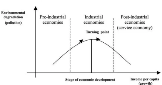
When analyzing the relationship of per capita income to air pollution per capita, a nonlinear relationship similar to Kuznet's U-hypothesis has been noted. This relationship shows that a country's early economic development degrades the environment until what is called the turning point is reached, after which the environment improves with further economic development. This relationship is referred to as the environmental Kuznets curve (Grossman & Krueger, 1995).

(9)

Figure 1 Environmental Kuznets Curve

There is little evidence to validate the inverted U ratio that EKC predicts (Stern, 2004), and a typical and predictable relationship between per capita income and pollution is questionable (Copeland & Taylor, 2003).

In cases where a relationship comparable to what EKC predicts is noticed, there may be underlying reasons for why the relationship arises, and this means that one cannot apply EKC as a general theory to the development of all countries. The underlying reasons of why an inverted U-relationship is noticed may be due to trade between countries and the fact that developed countries generally have more environmental regulations compared to developing countries. According to the Heckscher-Ohlin trade theory, countries will specialize in their production to goods whose factors they are relatively abundant in and then trade the excess of those goods with other countries. Developed countries are predicted to produce goods that require relatively more labor and capital, while developing countries are predicted to produce goods that require more labor. Since different types of productions have different effects on the environment, this specialization may be one of the reasons why the inverted U-ratio is noticed (Stern, 2004).

2.1.2 Revised Environmental Kuznets Curve

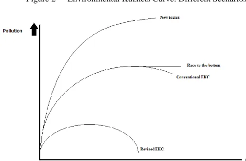
Dasgupta et al. (2002) presented an alternative view of the EKC, where he explains four different views on the relationship between pollution and income, which are seen in Figure 2.

(10)

Figure 2 Environmental Kuznets Curve: Different Scenarios

The different scenarios exist because the burden of proof for the original EKC is flawed. Two pessimistic views are referred to as race to the bottom and New toxic. The idea of the race to the bottom is that some critics of the EKC claim that globalization causes the emission levels to rise and stay at the absolute maximum level in a so-called "race to the bottom" of the environmental standard. Other pessimistic critics argue that the original EKC relationship may be right for some emissions. However, with economic development, new emissions will be created, which will mean that absolute emissions always rise with economic development, which is referred to as New Toxic. A more optimistic view is that of the Revised EKC, where it is assumed that the developed countries' innovations have a positive spillover effect in today's developing countries. This spillover effect and the liberalization that has taken place in developing countries in recent decades means more efficient handling of inputs and that environmentally hazardous activities are subsidized to a lesser degree. This spillover effects and liberalization leads that today's developing countries will have a lower peak level of environmental degradation than today's developed countries had (Dasgupta et al., 2002).

(11)

Stern (2004) considered that the relationship between emissions and per capita income is probably a mixture of two different scenarios that Dasgupta et al. (2002) called New Toxics and Revised EKC.

2.2 Previous empirical studies

After Grossman & Kreuger introduced the EKC in 1995, a lot of studies have been done on the EKC. One of the most known is the critique in Stern (2004). Stern’s critiques were that the EKC was weak in terms of econometrics. Stern argues that there wasn’t taking enough of consideration of possible problems with either stochastic trends or time series. The conclusion from Stern is that the evidence of the EKC is that it is statistically weak for the inverted U-shape (Stern, 2004).

Furthermore, in 2004 the EKC was reviewed by Dinda. This study by Dinda was looking at different previous studies on the EKC and the inverted U-shape. With the goal of proving if the theory of EKC holds or not. The findings of Dinda are that in countries' early stages of economic development, the focus on the climate is lower than in later stages of their economic development. That proves the main standpoint of the EKC. However, the result also shows that the turning point is not consistent; it varies a lot across studies for the same indicators. Another founding is that when countries become more economically developed, the productions tend to be outsourced to less developed countries with less interest in the climate. (Dinda, 2004)

Another study by Shahbaz and Sinha (2019), surveyed previous empirical papers were done on EKC and CO2. One of the main reasons for their paper is when MICs are

developing into developed countries, their need for electricity is increasing, and with increased energy consumption, the CO2 emissions generally increase. The main findings

of Shahbaz and Sinha conclude that there is a lack of studies that include the height of the EKCs. One question to be answered is if there is any turning-point beyond certain levels of CO2 emissions.

(12)

2.3 Hypothesis

The hypothesis to be tested is:

1) Middle-income and high-income countries' economic development between 1960 and 2014 is correlated with the CO2 emissions rate according to the

Environmental Kuznets curves predictions.

2) Middle-income countries have an, on average, lower and earlier turning point than high-income countries.

These hypotheses reflect the environmental Kuznets Curve, which is an economic theory that will be examined in this paper. The first hypothesis will test if the variables are correlated and if so, does the relationship follow the curve predicted by economic theory. The selection of focusing the paper on CO2 emissions is both because it is the greenhouse

emission that contains the foremost data and the fact that CO2 emissions are one of the

foremost vital contributors to global climate change (Houghton et al. 2001).

The second hypothesis tests if middle-income countries have transitioned to low carbon growth and development paths earlier compared to developed countries.

(13)

3. Empirical Framework

_____________________________________________________________________________________ In this section, we will present the data set and the variables used in the empirical tests in section 4 as well as the models. This section will also provide descriptive statistics.

______________________________________________________________________

3.1 Methodology

The environmental Kuznets curve theory predicts that emissions per capita initially have a positive correlation with GDP per capita. However, after a certain level of GDP per capita, the relationship becomes negative. Hence the theory predicts an inverted U-shape. The Environmental Kuznets curve postulates a nonlinear relationship between income and pollution. To test the first hypothesis, we follow the empirical studies on the EKC using the following model:

𝑌𝑖𝑡 = α 𝑖 + 𝛽0𝑋𝑖𝑡+ 𝛽1X2𝑖𝑡+ 𝜀𝑖𝑡 (Dinda, 2004). (1)

Where Yit is pollution per capita, Xit is the income per capita, and X2it is the income per

capita squared. αiis the intercept, β0 and β1 are the coefficients of the independent

variables. The εit is the error term that captures the variation in Yit that is not explained

by Xit or X2it. While i is 1,2,3…n countries and t is 1,2,3…t years. If β0 >0 and β1<0, the

EKC relationship between pollution per capita and income per capita would exist.

The second hypothesis: MIC: s has an, on average, lower turning point than high-income countries. We will use the coefficient retrieved from the regression one in order to calculate the predicted maximum of emissions, i.e., the turning point for the different panels. The turning point is calculated as:

𝑇 = (− 𝛽1

2𝛽2) (Dinda, 2004) (2)

According to our hypothesis, the turning point calculated by equation 2 will be significantly lower for MIC’s compared to HIC’s.

The data used in the empirical research are annual data estimated for the years available for each country with a max period of 1960-2014, hence a maximum of 54 observations per variable for each country. The variables used are GDP per capita (constant 2010 US$) and CO2 emissions per capita, and both are collected from the World Bank. GDP per

(14)

constant 2010 U.S. dollars value. CO2 emissions per capita are measured in tons of carbon

per capita, which is calculated from fossil fuel consumption and cement production. Fuels delivered to ships and aircraft in international transport are excluded from the calculations due to difficulties in distributing the fuels among the different countries.

The first step is to divide the countries into panel data. We will make panel data for high-income countries and middle-high-income countries for an aggregate comparison between the different classifications of countries. We need to be sure we can perform a regression of the variables without it being a spurious regression. To check that the regressions are not spurious, we will need to conduct some tests. First, will we conduct a panel cointegration test to decide whether the time series variables in the panel are stationarity or not. Further, a test to check if the variables are correlated or not will be performed. It will be tested with panel cointegration tests, which is a test that analyses the long-run relationship between the variables. If the variables are non-stationary at level and become stationary after equal amounts of difference and then share a long-run relationship, the regression will not be spurious.

3.2 Descriptive Statistics

The World Bank classifies countries based on their income levels. Currently, there are four different classifications: Low-income countries, Lower-middle-income countries, Upper-middle-income countries, and High-income countries. The income levels are measured by gross national income (GNI) per capita, in U.S. dollars, converted from the local currency, and the country classification is updated once a year.1_{We have used the}

World Bank's latest classification for our data, and we have merged Lower-middle-income countries and Upper-middle-Lower-middle-income countries into what we call middle-Lower-middle-income countries. A full list of which countries belong to the different classifications can be seen in Appendix 1.

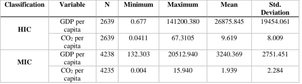
In Table 1, the descriptive statistics for HIC and MIC can be found. The values of the variables GDP per capita and CO2 per capita differ dramatically between HIC and MIC countries. Interestingly HIC has a lower minimum GDP per capita compared to MIC,

(15)

which is due to the World Bank classifies countries based on gross national income per capita, which may differ GDP per capita very much. The maximum and mean values for both variables are higher in the HIC countries. Still, the high standard deviation in all variables means that it differs a lot even between countries in the same classification.

Table 1 Descriptive Statistics aggregate HIC and MIC

Classification Variable N Minimum Maximum Mean Std. Deviation HIC GDP per capita 2639 0.677 141200.380 26875.845 19454.061 CO2 per capita 2639 0.0411 67.3105 9.619 8.009 MIC GDP per capita 4238 132.303 20512.940 3240.369 2751.451 CO2 per capita 4235 0.004 15.940 1.939 2.284

(16)

4. Results

_____________________________________________________________________________________ This section will provide the result from the empirical tests, which have been conducted in line with the empirical framework provide in section 3.

______________________________________________________________________

All tests presented in the paper are done in E-views, and full details of all the tests can be found in the Appendices.

4.1 Test to determine the econometric model

Before we can investigate the relationship between the independent variables and the dependent variable in Equation 1, we must first examine whether the variables are stationary or not. If all the variables are non-stationary, then we cannot be sure of the result from the OLS-regression is correct because of the risk that it is a spurious regression. A spurious regression is when one regresses a non-stationary variable on another non-stationary variable(s). Even if a long-term relationship doesn't exist between the variables, a spurious regression has the consequence that the relationship between the variables can be significant anyhow due to either coincidence or some other factor not included in the regression (Granger and Newbold, 1974). To avoid a false regression, we examine the variables through a panel root test.

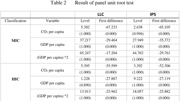
Table 2 Result of panel unit root test

LLC IPS

Classification Variable Level First difference Level First difference

MIC CO2 per capita 5.382 -67.233 2.638 -65.105 (1.000) (0.000) (0.996) (0.000) GDP per capita 37.217 -29.464 27.949 -35.372 (1.000) (0.000) (1.000) (0.000) (GDP per capita) ^2 65.247 -17.204 44.763 -29.761 (1.000) (0.000) (1.000) (0.000) HIC CO2 per capita 5.395 -55.599 3.392 -52.306 (1.000) (0.000) (1.000) (0.000) GDP per capita 1.228 -27.887 9.222 -27.119 (0.890) (0.000) (1.000) (0.000) (GDP per capita) ^2 13.913 -25.962 18.057 -25.882 (1.000) (0.000) (1.000) (0.000)

Note: The lag selection for every variable is based on Akaike Info Criterion. LLC and IPS tests for all the series include a constant as an intercept.

(17)

A panel unit root test is not the same as a unit root test for a time series data. There are two different types of panel unit root tests, common unit root process, and individual unit root process. Levin, Lin, and Chu (2002) use the common unit root process, which holds that the persistence parameters are standard across cross-sections. Im, Pesaran, and Shin (2003) use the individual unit root process, which instead assumes that the persistent parameters move freely across cross-sections. To be sure of the stationarity of the variables, we use both the test formulated by Levin, Lin, and Chu (LLC) and the one formulated by Im, Pesaran, and Shin (IPS). The results representing these tests can be found in Table 3, where they are presented for MIC and HIC. Table 3 shows that at a significance level of one percent that both tests show that all variables for both MIC and HIC are non-stationary and that it becomes stationary after the first difference.

Since the panel unit root test showed that the variables are non-stationary and that they become stationary after the first difference, we performed a panel integration test to investigate the long-term relationship between the variables. We have chosen to use two different panel integration tests, one test introduced by Pedroni (1999) and another test developed by Maddala and Wu (1999), which is referred to as the Johansen Fisher panel integration test.

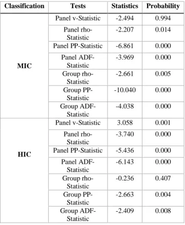
Pedroni (1999) derives seven different panel test statistics. Of these seven statistics, four are based on within-dimension, and three are based on between-dimension. Both the within‐dimension statistics and between‐dimension statistics have a null hypothesis of no cointegration for the panel and an alternative hypothesis of cointegration for the panel. In table 3, the Pedroni residual cointegration test is presented for MIC and HIC. Both for MIC and HIC, the null hypothesis is rejected in 6 out of 7 tests. Hence, we assume that there is cointegration of the variables in the panel.

(18)

Table 3 Results Pedroni residual cointegration test for equation 1

Classification Tests Statistics Probability

MIC Panel v-Statistic -2.494 0.994 Panel rho-Statistic -2.207 0.014 Panel PP-Statistic -6.861 0.000 Panel ADF-Statistic -3.969 0.000 Group rho-Statistic -2.661 0.005 Group PP-Statistic -10.040 0.000 Group ADF-Statistic -4.038 0.000 HIC Panel v-Statistic 3.058 0.001 Panel rho-Statistic -3.740 0.000 Panel PP-Statistic -5.436 0.000 Panel ADF-Statistic -6.143 0.000 Group rho-Statistic -0.236 0.407 Group PP-Statistic -2.663 0.004 Group ADF-Statistic -2.409 0.008

Table 4 Results Johansen Fisher panel cointegration test for equation 1

Hypothesized Fisher Stat Fisher Stat

Classification No. of CE(s) (from trace test) Prob. (from max-eigen test) Prob MIC None 1045.446 0.000 880.511 0.000 At most 1 406.616 0.000 358.023 0.000 At most 2 304.313 0.000 304.313 0.000 HIC None 517.871 0.000 436.748 0.000 At most 1 207.082 0.000 171.732 0.001 At most 2 189.065 0.000 189.065 0.000

The Johansen Fisher test developed by Maddala and Wu (1999) is testing both for the number of cointegration vectors and individual cointegration for the different cross‐ sections. The results of the Johansen Fisher panel cointegration test can be found in Table 4. To not make the table to big, we have chosen only to include the tests of the number cointegration vectors in Table 4, and the test of individual cointegration for the different cross‐sections can be found in the appendix. The tests of the number cointegration vectors have a null hypothesis of at most r cointegration vector. The null hypothesis is rejected on the level of at most two cointegration vectors for both MIC and HIC, which states that

(19)

there are more than two cointegrated vectors in our variables. Hence, a long-run relationship exists between more than two of our variables, which makes it possible for us to regress all our variables without the regression being spurious.

Since it was found that the variables are cointegrated, the next step before we can estimate long-run coefficients for the independent variables is to determine if we should use the random effect model (REM), Fixed effect model (FEM) or Pooled OLS model for our panel data regression. With the Pooled OLS model, one neglects the cross-section and time-series nature of the data and estimates an aggregate regression by pooling all observations. In the fixed-effect model, one also pools the observation but either allows for each cross-section unit to have its own intercept through the use of dummy variables or express each unit’s variable as a deviation from its mean value. The random effect model assumes that each unit has its own intercept value that is a random drawing from a population of units.

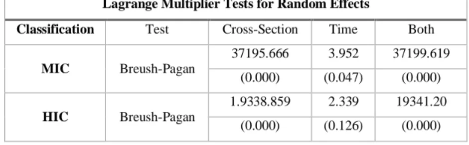
To test which estimation technique to use, we will first use the Lagrange Multiplier Tests for Random Effects, which is a group of tests that all originated from Breusch-Pagan (1980). The null hypothesis of the test is that the variance of the random effect is zero, and one should use Pooled OLS against the alternative hypothesis that the variance of the random effect is larger than zero and should use REM. Secondly, we investigate if REM appropriate by using a test by Hausman (1978). The null hypothesis of the Hausman test is that REM is suitable against the alternative hypothesis that REM is not suitable.

Table 5 Lagrange Multiplier Tests for Random Effects

Lagrange Multiplier Tests for Random Effects

Classification Test Cross-Section Time Both

MIC Breush-Pagan 37195.666 3.952 37199.619 (0.000) (0.047) (0.000) HIC Breush-Pagan 1.9338.859 2.339 19341.20 (0.000) (0.126) (0.000)

(20)

Table 6 Correlated Random Effects - Hausman Test

Correlated Random Effects - Hausman Test

Classification Test Summary Chi-Sq. Statistic Chi-Sq. d.f. Prob.

MIC Cross-section random 7.451 2 (0.024)

HIC Cross-section random 11.555 2 (0.003)

The result from the tests can be found in Tables 6 and 7. For both MIC and HIC, the result of the Lagrange multiplier test states that at a one percent significance level, REM is preferred to pooled OLS for cross-section while pooled OLS is preferred to REM for time. Hence, we need to test cross-section in the Hausman test to decide if one should use REM or FEM. For both MIC and HIC, the significance level is quite low, and the null hypothesis is rejected at 5% and 1% significance level, respectively. Hence, we chose to regress both MIC and HIC with cross-sectional fixed effects.

4.2 First hypothesis

Middle-income and high-income countries' economic development between 1960 and 2014 is correlated with the CO2 emissions rate according to the Environmental Kuznets

curves predictions.

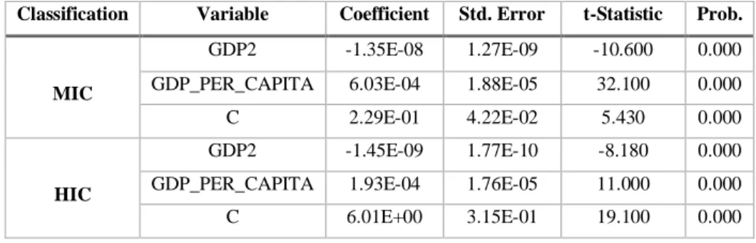
The results from the regression of equation one using FEM can be found in table 7. According to the results, the coefficient on GDP per capita is positive and statistically significant, and the coefficient on squared GDP per capita (GDP2) is negatively significant, which is in line with our first hypothesis. As seen in Table 7, at a low level of GDP per capita, an increase in GDP per capita increases the CO2 emission per capita, but

after a certain point, a further increase in GDP per capita decreases CO2 emission per

capita, which is the relationship that the EKC predicts.

Table 7 Results of regression for equation 1 using Least Squares FEM

Classification Variable Coefficient Std. Error t-Statistic Prob.

MIC

GDP2 -1.35E-08 1.27E-09 -10.600 0.000

GDP_PER_CAPITA 6.03E-04 1.88E-05 32.100 0.000

C 2.29E-01 4.22E-02 5.430 0.000

HIC

GDP2 -1.45E-09 1.77E-10 -8.180 0.000

GDP_PER_CAPITA 1.93E-04 1.76E-05 11.000 0.000

(21)

Serial correlation is common in multi-country GDP series due to dependence arising from global shocks and other more complicated interdependencies (Phillips and Moon, 1999). Because of the risk of serial correlation, we will also regress the equation using a fully modified least square (FMOLS) estimation method developed by Phillips and Moon (1999), which is estimated with a non-parametric approach that includes the alterations to tackle the serial correlation. By including a second approach for the regression, we are adding extra support to reject or accept the null hypothesis.

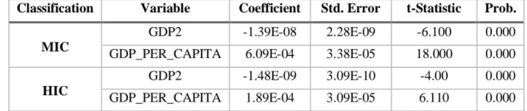
The results of equation 1 using FMOLS can be found in table 8, and we see that the results using FMOLS are very similar to using Least Squares with a fixed-effect model for cross-section seen in table 7. The coefficients for the variables using FMOLS are between -3% and + 3% compared to coefficients for the variables using the Least Squares with a fixed-effect model for cross-section.

Table 8 Results of regression for equation 1 using FMOLS

Classification Variable Coefficient Std. Error t-Statistic Prob. MIC

GDP2 -1.39E-08 2.28E-09 -6.100 0.000

GDP_PER_CAPITA 6.09E-04 3.38E-05 18.000 0.000 HIC

GDP2 -1.48E-09 3.09E-10 -4.00 0.000

GDP_PER_CAPITA 1.89E-04 3.09E-05 6.110 0.000

4.3 Second hypothesis

Middle-income countries have an, on average, lower and earlier turning point than high-income countries.

Before we can calculate the turning point for MIC and HIC, we want to know that the predicted regression lines are significantly different from each other. To do this, we have regressed all countries aggregated using equation 1 with cross-sectional fixed effects and dummy variable (D1) for MIC. The result from the regression can be found in Table 9, and in the table, we see that each variable is statistically significant, which means that the regression lines are significantly different for MIC and HIC.

(22)

Table 9 Results of regression for equation 1 using Least Squares FEM with dummy

Variable Coefficient Std. Error t-Statistic Prob. GDP_PER_CAPITA 1.93E-04 1.12E-05 17.324 0.000 GDP2 -1.45E-09 1.12E-10 -12.897 0.000 GDP_PER_CAPITA*D1 4.10E-04 6.99E-05 5.858 0.000 GDP2*D1 -1.21E-08 4.68E-09 -2.579 0.000

C 2.449 0.123 19.991 0.000

To calculate the turning point for MIC and HIC, we use equation 2 with the coefficient from Table 7 and Table 8.

𝑇𝑢𝑟𝑛𝑖𝑛𝑔 𝑝𝑜𝑖𝑛𝑡 𝑜𝑓 𝑡ℎ𝑒 𝐸𝐾𝐶 𝑓𝑜𝑟 𝑀𝐼𝐶 𝑢𝑠𝑖𝑛𝑔 𝑟𝑒𝑠𝑢𝑙𝑠𝑡 𝑓𝑟𝑜𝑚 𝑡𝑎𝑏𝑙𝑒 7 = 6.03𝐸 − 04 2 ∗ −1.35𝐸 − 08= $22 301 𝑇𝑢𝑟𝑛𝑖𝑛𝑔 𝑝𝑜𝑖𝑛𝑡 𝑜𝑓 𝑡ℎ𝑒 𝐸𝐾𝐶 𝑓𝑜𝑟 𝐻𝐼𝐶 𝑢𝑠𝑖𝑛𝑔 𝑟𝑒𝑠𝑢𝑙𝑠𝑡 𝑓𝑟𝑜𝑚 𝑡𝑎𝑏𝑙𝑒 7 = 1.93𝐸 − 04 2 ∗ −1.45𝐸 − 09= $66 786 𝑇𝑢𝑟𝑛𝑖𝑛𝑔 𝑝𝑜𝑖𝑛𝑡 𝑜𝑓 𝑡ℎ𝑒 𝐸𝐾𝐶 𝑓𝑜𝑟 𝑀𝐼𝐶 𝑢𝑠𝑖𝑛𝑔 𝑟𝑒𝑠𝑢𝑙𝑠𝑡 𝑓𝑟𝑜𝑚 𝑡𝑎𝑏𝑙𝑒 8 = 6.09𝐸 − 04 2 ∗ −1.39𝐸 − 08= $21 916 𝑇𝑢𝑟𝑛𝑖𝑛𝑔 𝑝𝑜𝑖𝑛𝑡 𝑜𝑓 𝑡ℎ𝑒 𝐸𝐾𝐶 𝑓𝑜𝑟 𝐻𝐼𝐶 𝑢𝑠𝑖𝑛𝑔 𝑟𝑒𝑠𝑢𝑙𝑠𝑡 𝑓𝑟𝑜𝑚 𝑡𝑎𝑏𝑙𝑒 8 = 1.89𝐸 − 04 2 ∗ −1.48𝐸 − 09= $63 632

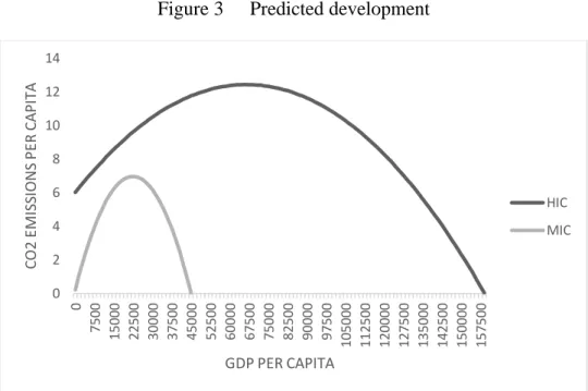
The calculations state that MIC CO2 emissions will decrease once GDP per capita

reaches $21916 - $22301, which is much earlier compared to HIC that has a turning point at GDP per capita of $63632 - $66786. By calculating the CO2 emission at the

respective turning point using the regression of the Least Squares Fixed effects model in Table 7 we also find the maximum level of CO2 emissions. For MIC, the CO2 emission

reaches 6.96 metric tons of carbon per capita, and for HIC, it reaches 12.43 metric tons of carbon per capita. A visualization of the relationship between CO2 emission per

capita and GDP per capita based on the results in Table 7 is shown in Figure 3. In the graph one clearly sees that the different relationship for MIC and HIC is in line with our second hypothesis.

(23)

Figure 3 Predicted development 0 2 4 6 8 10 12 14 0 7500 ₁₅₀₀₀ ₂₂₅₀₀ ₃₀₀₀₀ ₃₇₅₀₀ ₄₅₀₀₀ ₅₂₅₀₀ ₆₀₀₀₀ ₆₇₅₀₀ ₇₅₀₀₀ ₈₂₅₀₀ ₉₀₀₀₀ ₉₇₅₀₀ 105000 112500 120000 127500 135000 142500 150000 157500 C O 2 EMI SS IO N S P ER C A P IT A GDP PER CAPITA HIC MIC

(24)

5. Analysis

_____________________________________________________________________________________ This section will analysis the results in section 4, in line with the theoretical framework in section 2.

______________________________________________________________________

The first empirical test of this paper was the correlation between economic development and CO2 emission from 1960 to 2014. The test was divided between all 107 middle- and

all 77 high-income countries, according to the World Bank. The middle-income are all merged from the World Banks' lower- and upper-middle-income countries. The GDP per capita was used as the explanatory variable and CO2 emissions per capita the response;

this in line with the EKC from Grossman and Kreuger (1995). The theory of EKC predicts that in the early stages of an economy’s development, CO2 emissions will increase until

a certain level of what is called the turning point, after which further economic development has a negative effect on the CO2 emission. This will be formed as an inverted

U-shape. The result was as expected, and it confirms the EKC inverted U-shape for both MIC’s and HIC’s.

The second empirical test of our paper tests whether the relationship is similar to what the Revised EKC by Dasgupta et al. (2002) assume. The theory assumes that middle-income countries, on average, have a lower and earlier turning point than high-middle-income countries. The Revised EKC suggests that countries that are later in their economic development have a lower turning point of the inverted U-shape than already developed countries. The result of the test showed a significantly lower turning point average for MIC’s compared to HIC’s both at a 1 percent level of significance. If all these countries have reached the turning-point is something that is not tested for. Hence the numbers are just an average based on a panel-test.

In section 2.1.2, the Revised EKC is discussed and the two pessimistic views, race to the bottom and new toxic. Dasgupta questions if CO2 emission is replaced by other emissions

when GDP per capita increases. However, this is difficult to study since, in many countries, other types of emissions are not recorded as the CO2 emissions. Hence data on

them is lacking. That lacking data of other emissions is the reason why this paper only tests for CO2.

(25)

The EKC is a highly debatable theory were some scholars criticize the whole existence of it and while others argue that it follows another path, where the race to the bottom scenario is one of the most known. This scenario argued by Dinda (2004), is that while HIC controls their emissions with cost heavily regulations, the incentive for firms in HIC’s is to outsource their production to less-developed countries. In the less-developed countries, the priority is on jobs and economic development rather than clean air and pollution.

Outsourced production increases trade, and several studies have been studying trade openness and its relationship to CO2 emissions. Atci (2009) researched this relationship

in four countries throughout 22 years. The result was that trade openness had a negative impact on CO2 emissions. That could be one factor why further developed countries can

lower their CO2 emissions while it is increasing in less developed. The less developed

countries transformation from agricultural to industry. According to Shao et al. (2014), there is a positive correlation between industrialization, urbanization, and energy consumption. The environmentally friendly energy cannot compete in terms of price with fossil fuel energy. Therefore, expensive low carbon energy will not be used by less developed countries.

As mentioned earlier, this study was conducted on a total of 184 countries, divided into only two panels, and only three variables GDP per capita, GDP per capita squared, and CO2 per capita. While our study shows confirmation of the EKC and the Revised EKC,

the result needs to be taken with caution due that the study was only dividing the countries into two different economic stages while using only two independent variables. It could be other differences that explain the economic development and CO2 emissions, such as

region, sociological factors, size of the country, natural resources, other emissions, export, and import. The main overall reason why only these variables are used is due to a lack of data. The only emission World Bank has for all these countries from the 1960s is CO2 emissions. Furthermore, the impact of import and export is something that is hard to

count. Do the emissions from the production count in the imported goods, or does it count as the production country’s emissions? Nonetheless, we did try to divide the countries into different regions based on the World Banks' different classifications. Somehow, we did not manage to test this econometrically, mostly due to a problem with spurious

(26)

regressions. Due to these complex situations, we decided to use the data provided by the World Bank and fewer variables.

(27)

6. Conclusion

Two different questions have been tested in this paper. The first question tested the Environmental Kuznets Curve’s existence in the middle- and high-income countries. The middle-income countries are the World Bank’s two groups of low- and upper-middle economies. The high-income countries are the economies that World Bank classifies as high-income or OECD. The test was conducted throughout the years between 1960-2014 and the three variables CO2, GDP, and GDP2, was used. The result confirmed the

existence of the EKC and the inverted-U shape for both middle- and high-income countries, all at a 1 percent level of significance.

The second empirical question of this study was if the turning point on the Revised Environmental Kuznets Curve is significantly lower for middle-income countries compared to high-income countries. The data was the same as for the first test. The result confirmed that the turning point for middle-income countries was significantly lower, all at a one percent level of significance. We did test this panel data with both FMOLS and Fixed effect models. The result was similar for both tests. The average turning point for middle-income countries was approximately $22 000 per capita, while for high-income countries, approximately $64 000 per capita. 2010 is used as the constant for GDP per capita.

This leaves room for many further studies. Once the turning point has been reached, do other emissions increase while CO2 decreases? Could there be other factors than GDP per

capita that affects CO2 emissions? For example, countries' energy sources, sociological

factors, or natural resources. These are all interesting variables that we could see have an impact on the CO2 emissions and Environmental Kuznets Curve.

(28)

Reference list

Alonso, J., Glennie, J. and Sumner, A., 2014. Recipients and Contributors: Middle income countries and the future of development cooperation. Department of Economic & Social Affairs.

Breusch, T. and Pagan, A., 1980. The Lagrange Multiplier Test and its Applications to Model Specification in Econometrics. The Review of Economic Studies, 47(1), p.239. Canadell, J., Le Quere, C., Raupach, M., Field, C., Buitenhuis, E., Ciais, P., Conway, T., Gillett, N., Houghton, R. and Marland, G. (2007). Contributions to accelerating atmospheric CO2 growth from economic activity, carbon intensity, and efficiency of natural sinks. Proceedings of the National Academy of Sciences, 104(47).

Chakraborty, B. (2017). Paris Agreement on climate change: US withdraws as Trump calls it 'unfair'. Fox News. Available at: https://www.foxnews.com/politics/paris-agreement-on-climate-change-us-withdraws-as-trump-calls-it-unfair [Accessed 4 Feb. 2020].

Copeland, B. and Taylor, M., 2003. Trade, growth and the environment. National bureau of economic research.

Dasgupta, S., Laplante, B., Wang, H., & Wheeler, D. (2002). Confronting the environmental Kuznets curve. Journal of Economic Perspectives, 16, 147–168.

Datahelpdesk.worldbank.org. 2020. How Does The World Bank Classify Countries? – World Bank Data Help Desk. [online] Available at: <https://datahelpdesk.worldbank.org/knowledgebase/articles/378834-how-does-the-world-bank-classify-countries> [Accessed 8 April 2020].

Dinda, S., 2004. Environmental Kuznets Curve Hypothesis: A Survey. Ecological Economics, 49(4), pp.431-455.

Gene M. Grossman and Alan B. Krueger. (1991). Environmental impacts of a north american free trade agreement. National bureau of economic research.

Granger, C. and Newbold, P., 1974. Spurious regressions in econometrics. Journal of Econometrics, 2(2), pp.111-120.

Grossman, G.M., Krueger, A.B. (1995), Economic growth and the environment, Quarterly Journal of Economics, Volume 110 353–377.

Houghton, J.T., Ding, Y., Griggs, D.J., Noguer, M., van der Linden, P.J., Dai, X., Maskell, K., Johnson, C.A. (2001). Climate change 2001: The Scientific Basis. Cambridge: Cambridge university press.

Im KS, Pesaran MH, Shin Y. Testing for unit roots in heterogeneous panels. Journal of Econometrics 2003; 115: 53–74.

(29)

IPCC, 2007: Summary for Policymakers. In: Climate Change 2007: The Physical Science Basis. Contribution of Working Group I to the Fourth Assessment Report of the Intergovernmental Panel on Climate Change [Solomon, S., D. Qin, M. Manning, Z. Chen, M. Marquis, K.B. Averyt, M.Tignor and H.L. Miller (eds.)]. Cambridge University Press, Cambridge, United Kingdom and New York, NY, USA.

Kapuria-Foreman, V., Perlman, M. (1995), An Economic Historian’s Economist: Remembering Simon Kuznets, The economic journal, Volume 105 (November,) 1524-1547.

Khan, M., Khan, M. and Rehan, M. (2020). The relationship between energy consumption, economic growth and carbon dioxide emissions in Pakistan. Financial Innovation, 6(1).

Kuznets, S. (1955). Economic Growth and Income Inequality. The American Economic Review, 45(1), 1-28. Retrieved February 26, 2020, from www.jstor.org/stable/1811581. Levin, A., Lin, C. and James Chu, C., 2002. Unit root tests in panel data: asymptotic and finite-sample properties. Journal of Econometrics, 108(1), pp.1-24.

Lorente, D. and Álvarez-Herranz, A. (2016). Economic growth and energy regulation in the environmental Kuznets curve. Environmental Science and Pollution Research, 23(16), pp.16478-16494.

Maddala, G. S. and Wu, S. (1999), “A Comparative Study of Unit Root Tests with Panel Data and A New Simple Test”, Oxford Bulletin of Economics and Statistics 61, 631–652. Millennium Ecosystem Assessment, 2005. Ecosystems and Human Well-being: Synthesis. Island Press, Washington, DC

Novus Group International AB (2019). Viktigaste politiska frågan. Novus Group International AB. Available at: https://novus.se/wp-content/uploads/2019/11/novusviktigastefrganov2019.pdf [Accessed 4 Feb. 2020]. Osborne, T. and Kiker, C. (2005). Carbon offsets as an economic alternative to large-scale logging: a case study in Guyana. Ecological Economics, 52(4), pp.481-496.

Panayotou, T., 1993. Empirical Tests and Policy Analysis of Environmental Degradation at Different Stages of Economic Development. Empirical Tests and Policy Analysis of Environmental Degradation at Different Stages of Economic Development.

Pedroni P. Critical values for cointegration tests in heterogeneous panels with multiple regressors. Oxf Bull Econ Stat 1999; 61: 653–670.

Phillips, P. and Moon, H., 1999. Linear Regression Limit Theory for Nonstationary Panel Data. Econometrica, 67(5), pp.1057-1111.

(30)

Romani, M., Rydge, J. and Stern, N., 2012. Recklessly slow or a rapid transition to a low-carbon economy? Time to decide. Centre for Climate Change Economics and Policy Grantham Research Institute on Climate Change and the Environment.

Shahbaz, M. and Sinha, A., 2019. Environmental Kuznets curve for CO2 emissions: a literature survey. Journal of Economic Studies.

Shao, C., Guan, Y., Wan, Z., Guo, C., Chu, C. and Ju, M. (2014). Performance and decomposition analyses of carbon emissions from industrial energy consumption in Tianjin, China. Journal of Cleaner Production, 64, pp.590-601.

Steffen, W., Crutzen, P. and McNeill, J. (2007). The Anthropocene: Are Humans Now Overwhelming the Great Forces of Nature. AMBIO: A Journal of the Human Environment, 36(8), pp.614-621.

Social Science Research Solutions, Inc (2019). Available at: http://cdn.cnn.com/cnn/2019/images/04/29/rel6a.-.2020.democrats.pdf [Accessed 4 Feb. 2020].

Stern, D. (2004), The Rise and Fall of the Environmental Kuznet Curve, Elsevier Ltd, Volume 32, No 8, 1419-1439.

Tabellini, G., 2010. Culture and Institutions: Economic Development in the Regions of Europe. Journal of the European Economic Association, 8(4), pp.677-716.

United Nations Framework Convention on Climate Change. (1992). Available at: https://unfccc.int/files/essential_background/background_publications_htmlpdf/applicat ion/pdf/conveng.pdf [Accessed 19 Feb. 2020].

United Nations Framework Convention on Climate Change (2015). PARIS AGREEMENT. United Nations Framework Convention on Climate Change. Available at:

https://unfccc.int/files/essential_background/convention/application/pdf/english_paris_a greement.pdf [Accessed 4 Feb. 2020].

World Bank. 2020. Overview. [online] Available at: <https://www.worldbank.org/en/topic/poverty/overview> [Accessed 14 May 2020].

(31)

Appendix 1 Descriptive statistics

List of countries per classification

List of countries

MIC HIC

Papua New Guinea Australia

Cambodia Brunei Darussalam

Indonesia French Polynesia

Kiribati Guam

Lao PDR Hong Kong SAR, China

Micronesia, Fed. Sts. Japan

Mongolia Korea, Rep.

Myanmar Macao SAR, China

Philippines New Caledonia

Solomon Islands New Zealand

Timor-Leste Northern Mariana Islands

Vanuatu Palau

Vietnam Singapore

American Samoa Andorra

China Austria

Fiji Belgium

Malaysia Croatia

Marshall Islands Cyprus

Nauru Czech Republic

Samoa Denmark

Thailand Estonia

Tonga Faroe Islands

Tuvalu Finland

Kyrgyz Republic France

Moldova Germany Ukraine Gibraltar Uzbekistan Greece Albania Greenland Armenia Hungary Azerbaijan Iceland Belarus Ireland

Bosnia and Herzegovina Isle of Man

Bulgaria Italy

Georgia Latvia

Kazakhstan Liechtenstein

Kosovo Lithuania

Montenegro Luxembourg

North Macedonia Monaco

Romania Netherlands

Russian Federation Norway

(32)

Turkey Portugal

Turkmenistan San Marino

Peru Slovak Republic

Dominican Republic Slovenia

Bolivia Spain

El Salvador Sweden

Honduras Switzerland

Nicaragua United Kingdom

Argentina Antigua and Barbuda

Belize Aruba

Brazil Bahamas, The

Colombia Barbados

Costa Rica British Virgin Islands

Cuba Cayman Islands

Dominica Chile

Ecuador Panama

Grenada Puerto Rico

Guatemala Sint Maarten (Dutch part)

Guyana St. Kitts and Nevis

Jamaica St. Martin (French part)

Mexico Trinidad and Tobago

Paraguay Turks and Caicos Islands

St. Lucia Uruguay

St. Vincent and the Grenadines Virgin Islands (U.S.)

Suriname Bahrain

Venezuela, RB Israel

Djibouti Kuwait

Egypt, Arab Rep. Malta

Morocco Oman

Tunisia Qatar

West Bank and Gaza Saudi Arabia

Algeria United Arab Emirates

Iran, Islamic Rep. Bermuda

Iraq Canada

Jordan United States

Lebanon Seychelles Libya Pakistan Bangladesh Bhutan India Maldives Sri Lanka Congo, Rep. Nigeria Angola

(33)

Cabo Verde Cameroon Comoros Côte d'Ivoire Eswatini Ghana Kenya Lesotho Mauritania

São Tomé and Principe Senegal Sudan Zambia Zimbabwe Botswana Equatorial Guinea Gabon Mauritius Namibia South Africa

Descriptive statistics HIC

CO2_PER... GDP_PER... Mean 9.619112 26875.85 Median 7.590615 22758.41 Maximum 67.31050 141200.4 Minimum 0.041070 0.677431 Std. Dev. 8.009051 19454.06 Skewness 2.512521 1.378868 Kurtosis 12.16813 5.602818 Jarque-Bera 12019.08 1581.175 Probability 0.000000 0.000000 Sum 25384.84 70925355

Sum Sq. Dev. 169214.2 9.98E+11

(34)

Descriptive statistics MIC

Appendix 2 Cointegration tests

Pedroni residual cointegration test MIC

CO2_PER... GDP_PER... Mean 1.938719 3240.369 Median 1.036000 2433.462 Maximum 15.94028 20512.94 Minimum -0.020098 132.3032 Std. Dev. 2.283932 2751.451 Skewness 2.237629 1.842895 Kurtosis 8.816304 7.344604 Jarque-Bera 9510.307 5732.007 Probability 0.000000 0.000000 Sum 8216.290 13732682

Sum Sq. Dev. 22101.65 3.21E+10

Observations 4238 4238

Pedroni Residual Cointegration Test

Series: CO2_PER_CAPITA GDP2 GDP_PER_CAPITA Date: 03/17/20 Time: 13:08

Sample: 1960 2014 Included observations: 5885

Cross-sections included: 104 (3 dropped) Null Hypothesis: No cointegration Trend assumption: No deterministic trend

Automatic lag length selection based on SIC with lags from 0 to 10 Newey-West automatic bandwidth selection and Bartlett kernel Alternative hypothesis: common AR coefs. (within-dimension)

Weighted

Statistic Prob. Statistic Prob. Panel v-Statistic -2.493720 0.9937 -1.421620 0.9224 Panel rho-Statistic -2.206812 0.0137 -3.681580 0.0001 Panel PP-Statistic -6.860961 0.0000 -5.596426 0.0000 Panel ADF-Statistic -3.968685 0.0000 -5.338474 0.0000 Alternative hypothesis: individual AR coefs. (between-dimension)

Statistic Prob. Group rho-Statistic -2.660974 0.0039 Group PP-Statistic -10.04066 0.0000 Group ADF-Statistic -9.599644 0.0000

(35)

Pedroni residual cointegration test HIC

Johansen Fisher panel cointegration test MIC

Pedroni Residual Cointegration Test

Series: CO2_PER_CAPITA GDP_PER_CAPITA GDP2 Date: 03/17/20 Time: 13:12

Cross-sections included: 61 (16 dropped) Null Hypothesis: No cointegration Trend assumption: No deterministic trend

Automatic lag length selection based on SIC with lags from 2 to 10 Newey-West automatic bandwidth selection and Bartlett kernel Alternative hypothesis: common AR coefs. (within-dimension)

Weighted

Statistic Prob. Statistic Prob. Panel v-Statistic 3.058029 0.0011 2.071031 0.0192 Panel rho-Statistic -3.740038 0.0001 -3.711195 0.0001 Panel PP-Statistic -5.436143 0.0000 -3.812475 0.0001 Panel ADF-Statistic -6.144658 0.0000 -3.890565 0.0001 Alternative hypothesis: individual AR coefs. (between-dimension)

Statistic Prob. Group rho-Statistic -0.236129 0.4067 Group PP-Statistic -2.662465 0.0039 Group ADF-Statistic -2.408653 0.0080

Johansen Fisher Panel Cointegration Test

Series: CO2_PER_CAPITA GDP2 GDP_PER_CAPITA Date: 03/17/20 Time: 13:10

Trend assumption: Linear deterministic trend Lags interval (in first differences): 1 1

Unrestricted Cointegration Rank Test (Trace and Maximum Eigenvalue)

Hypothesized Fisher Stat.* Fisher Stat.*

No. of CE(s) (from trace test) Prob. (from max-eigen t... Prob.

None 1045. 0.0000 880.5 0.0000

At most 1 406.6 0.0000 358.0 0.0000

At most 2 304.3 0.0000 304.3 0.0000

(36)

Johansen Fisher panel cointegration test HIC

Appendix 3 Estimation technique tests

Lagrange Multiplier Tests for Random Effects HIC

Johansen Fisher Panel Cointegration Test

Series: CO2_PER_CAPITA GDP_PER_CAPITA GDP2 Date: 03/17/20 Time: 13:17

Trend assumption: Linear deterministic trend Lags interval (in first differences): 1 1

Unrestricted Cointegration Rank Test (Trace and Maximum Eigenvalue)

Hypothesized Fisher Stat.* Fisher Stat.*

No. of CE(s) (from trace test) Prob. (from max-eigen t... Prob.

None 517.9 0.0000 436.7 0.0000

At most 1 207.1 0.0000 171.7 0.0014

At most 2 189.1 0.0001 189.1 0.0001

* Probabilities are computed using asymptotic Chi-square distribution.

Lagrange Multiplier Tests for Random Effects Null hypotheses: No effects

Alternative hypotheses: Two-sided (Breusch-Pagan) and one-sided (all others) alternatives

Test Hypothesis

Cross-section Time Both

Breusch-Pagan 37195.67 3.952199 37199.62 (0.0000) (0.0468) (0.0000) Honda 192.8618 1.988014 137.7796 (0.0000) (0.0234) (0.0000) King-Wu 192.8618 1.988014 116.3193 (0.0000) (0.0234) (0.0000) Standardized Honda 196.3731 2.120791 132.3229 (0.0000) (0.0170) (0.0000) Standardized King-Wu 196.3731 2.120791 110.5726 (0.0000) (0.0170) (0.0000) Gourieroux, et al.* -- -- 37199.62 (0.0000)

(37)

Lagrange Multiplier Tests for Random Effects HIC

Lagrange Multiplier Tests for Random Effects Null hypotheses: No effects

Alternative hypotheses: Two-sided (Breusch-Pagan) and one-sided (all others) alternatives

Test Hypothesis

Cross-section Time Both

Breusch-Pagan 19338.86 2.339186 19341.20 (0.0000) (0.1262) (0.0000) Honda 139.0642 -1.529440 97.25178 (0.0000) (0.9369) (0.0000) King-Wu 139.0642 -1.529440 95.81604 (0.0000) (0.9369) (0.0000) Standardized Honda 142.7127 -1.439727 92.44649 (0.0000) (0.9250) (0.0000) Standardized King-Wu 142.7127 -1.439727 90.95720 (0.0000) (0.9250) (0.0000) Gourieroux, et al.* -- -- 19338.86 (0.0000)

(38)

Correlated Random Effects - Hausman Test MIC

Correlated Random Effects - Hausman Test Equation: Untitled

Test cross-section random effects

Test Summary Chi-Sq. Statistic Chi-Sq. d.f. Prob.

Cross-section random 7.451253 2 0.0241

Cross-section random effects test comparisons:

Variable Fixed Random Var(Diff.) Prob.

GDP_PER_CAPITA 0.000603 0.000609 0.000000 0.0093

GDP2 -0.000000 -0.000000 0.000000 0.0297

Cross-section random effects test equation: Dependent Variable: CO2_PER_CAPITA Method: Panel Least Squares

Date: 03/20/20 Time: 13:39 Sample: 1960 2014

Periods included: 55

Cross-sections included: 105

Total panel (unbalanced) observations: 4238

Variable Coefficient Std. Error t-Statistic Prob.

C 0.229004 0.042189 5.428069 0.0000

GDP_PER_CAPITA 0.000603 1.88E-05 32.11522 0.0000

GDP2 -1.35E-08 1.27E-09 -10.61993 0.0000

Effects Specification Cross-section fixed (dummy variables)

R-squared 0.920568 Mean dependent var 1.938719

Adjusted R-squared 0.918530 S.D. dependent var 2.283932 S.E. of regression 0.651903 Akaike info criterion 2.007081 Sum squared resid 1755.582 Schwarz criterion 2.167451 Log likelihood -4146.006 Hannan-Quinn criter. 2.063762 F-statistic 451.6569 Durbin-Watson stat 0.231775 Prob(F-statistic) 0.000000

(39)

Correlated Random Effects - Hausman Test HIC

Correlated Random Effects - Hausman Test Equation: Untitled

Test cross-section random effects

Test Summary Chi-Sq. Statistic Chi-Sq. d.f. Prob.

Cross-section random 11.555164 2 0.0031

Cross-section random effects test comparisons:

Variable Fixed Random Var(Diff.) Prob.

GDP_PER_CAPITA 0.000193 0.000201 0.000000 0.0214

GDP2 -0.000000 -0.000000 0.000000 0.2476

Cross-section random effects test equation: Dependent Variable: CO2_PER_CAPITA Method: Panel Least Squares

Date: 03/20/20 Time: 13:41 Sample: 1960 2014

Periods included: 55 Cross-sections included: 64

C 6.014593 0.315026 19.09238 0.0000

GDP_PER_CAPITA 0.000193 1.76E-05 10.98569 0.0000

GDP2 -1.45E-09 1.77E-10 -8.178620 0.0000

(40)

Appendix 4 Regression result

Regression result MIC using Least Squares fixed effects model

Regression result HIC using Least Squares fixed effects model

Dependent Variable: CO2_PER_CAPITA Method: Panel Least Squares

Date: 04/11/20 Time: 08:48 Sample: 1960 2014

Periods included: 55

GDP2 -1.35E-08 1.27E-09 -10.61993 0.0000

GDP_PER_CAPITA 0.000603 1.88E-05 32.11522 0.0000

C 0.229004 0.042189 5.428069 0.0000

Dependent Variable: CO2_PER_CAPITA Method: Panel Least Squares

Date: 04/11/20 Time: 08:54 Sample: 1960 2014

Periods included: 55 Cross-sections included: 64

GDP2 -1.45E-09 1.77E-10 -8.178620 0.0000

GDP_PER_CAPITA 0.000193 1.76E-05 10.98569 0.0000

C 6.014593 0.315026 19.09238 0.0000

(41)

Regression result MIC using FMOLS

Regression result HIC using FMOLS

Dependent Variable: CO2_PER_CAPITA

Method: Panel Fully Modified Least Squares (FMOLS) Date: 04/11/20 Time: 09:02

Sample (adjusted): 1961 2014 Periods included: 54

Total panel (unbalanced) observations: 4157 Panel method: Pooled estimation

Cointegrating equation deterministics: C

Coefficient covariance computed using default method

Long-run covariance estimates (Bartlett kernel, Newey-West fixed bandwidth)

GDP2 -1.39E-08 2.28E-09 -6.103328 0.0000

GDP_PER_CAPITA 0.000609 3.38E-05 18.03006 0.0000

Adjusted R-squared 0.919258 S.D. dependent var 2.289052 S.E. of regression 0.650437 Sum squared resid 1713.849 Long-run variance 1.293825

Dependent Variable: CO2_PER_CAPITA

Method: Panel Fully Modified Least Squares (FMOLS) Date: 04/11/20 Time: 09:06

Sample (adjusted): 1961 2014 Periods included: 54

Total panel (unbalanced) observations: 2580 Panel method: Pooled estimation

Cointegrating equation deterministics: C

Coefficient covariance computed using default method

Long-run covariance estimates (Bartlett kernel, Newey-West fixed bandwidth)

GDP2 -1.48E-09 3.09E-10 -4.799506 0.0000

GDP_PER_CAPITA 0.000189 3.09E-05 6.107135 0.0000

Adjusted R-squared 0.781598 S.D. dependent var 7.860563 S.E. of regression 3.673520 Sum squared resid 33966.28 Long-run variance 40.32930

Economic Development and CO2 emissons: A comparison of High- and Middle-income economies