Mean Residual Life Estimation Considering Operating Environment

Mean Residual Life Estimation Considering Operating

Environment

B. Ghodrati, F. Ahmadzadeh, U. Kumar Div. of Operation and Maintenance Engineering

Luleå University of Technology, Sweden behzad.ghodrati@ltu.se farzaneh.ahmadzadeh@ltu.se

uday.kumar@ltu.se

Abstract — The cost of maintenance of mechanized and

automated mining systems is too high necessitating efforts to enhance the effectiveness of maintenance systems and organization. For effective maintenance planning, it is important to have a good understanding of the reliability and availability characteristics of the systems. This is essential for determining the Mean Residual Life (MRL) of systems so that maintenance tasks could be planned effectively. In this paper we used the statistical approach to estimate MRL. A Weibull proportional hazard model (PHM) with time-independent covariates was considered for modelling of the hazard function so that operating environment could be integrated in the reliability analysis. Methods are presented for calculating the conditional reliability function and computing the MRL as a function of the current conditions to guarantee the desired output. The model is verified and validated using data from the Hydraulic system of an LHD fleet from a Swedish mine. The results obtained from the analysis is useful to estimate the remaining useful life of such system which can be subsequently used for effective maintenance planning and help controlling unplanned stoppages of highly mechanized and automated systems.

Keywords

—

Model, Conditional Reliability Function, Weibull Distribution, LHD Machine

I. INTRODUCTION

To cope with the technological advancement, mechanized and complex mining machinery like Load Haul Dump (LHD) are now being used in mining. The profitable introduction of such sophisticated capital intensive machines requires the achievement of the highest levels of reliability and availability during operation. Performance of a mining machine depends on the reliability of the equipment used and other factors. The machine reliability, maintainability and availability (RAM) assumed great significance in recent years due to competitive environment and overall operating /production cost [4].

High costs of maintaining complex equipment make it necessary to enhance maintenance support systems and changing traditional strategies by new ones like MRL which estimate time to failure for one or more existing and future failure modes. Then the prediction of a system's lifetime, whose objective is to predict the MRL before a failure occurs given the current machine condition and past operation profile [17]. Therefore, the reliability estimation of equipment as well

as its MRL is essential in maintenance optimization [6]. In recent years, MRL prediction in service has received increasing attention. It is important to assess the MRL of an asset while in use since it has impacts on the operational performance and profitability of an asset. When the failure indication has been detected, it is essential to estimate the MRL accurately for making a timely maintenance decision for failure avoidance. Likewise, more accurate reliability estimation is likely to result in accurate determining of the optimal inspection intervals, then minimizing the overall cost of the system [8, 11, and 19].

Nowadays MRL or Remaining Useful Life (RUL) is recognized as a key feature in maintenance strategies, while the real prognostic systems are rare in industry, even in mining industry. However the useful life is found variant depending on the actual operating conditions and characteristics of the environment such as temperature and pressure, humidity condition and corrosion rate, of course there are many uncertainties that might result in an inaccurate estimation of MRL as well. Therefore a central problem can be pointed out that the accuracy of a prognostic system is related to its ability to approximate and predict the degradation of equipment. However, in practice, choosing an efficient technique depends on classical constraints that limit the applicability of the tools, e.g. available data knowledge experiences, dynamic and complexity of the system, implementation requirements (precision, computation time, etc.), and available monitoring devices. Moreover, implementing an adequate tool can be a non-trivial task as it can be difficult to provide effective models of dynamic systems.

In this paper we utilize reliability methods to estimate the mean residual life at any given time t, then first we explain some theoretical point then follow it up by case study and use of reliability methods in determining the MRL as well as the optimal operating condition and for this ,we consider the following assumptions: (a) Best fit distribution for time to failure of mechanical components is Weibull distribution and for this at first we apply trend test and serial correlation test to be sure about the assumption of Independency and Identically Distribution (iid) of the data so that we can use the renewal process model like Weibull [10]; (b) System reliability characteristics and factors for both the component and the whole system are required for reliability analysis and MRL

estimation. Systems operating environmental factors such as dust, system temperature, operators’ skills (known as covariates) are assumed influencing covariate in this context according to [9].

II. STATISTICAL RELIABILITY ANALYSIS

The Cox's proportional hazard model [5] (PHM) is a complement to the set of tools use in reliability analysis and provides some particular advantageous features [10]. This model is classified as multiplicative and semi-parametric regression model considering covariates that assumes the hazard rate of a system/component is a product of baseline hazard rate, dependent on time only and a positive functional term f (z, α) = exp (zα) (we assume it has exponential form) basically independent of time, incorporating the effects of a number of covariates such as temperature, pressure and changes in design. It has been successfully used for survival analyses in medical areas and reliability predictions in the presence of external influencing factors Thus:

    n i i i z t z t z t 1 0 0( )exp( ) ( )exp( ) ) , (     

Where α (column vector) is the unknown parameter of the model or regression coefficient of the corresponding n covariates (z) indicating the degree of influence which each covariate has on the hazard function. One of the advantages of the PH model is its capability of including time-dependent and independent covariates. Kalbfleisch and Prentice (1980) classified the covariates into two broad categories internal and external covariates. An internal covariate is the output of a stochastic process generated by the unit under study and usually is time dependent. It can be observed as long as the unit survives and is not censored. On the other hand, an external covariate which can be time independent in general could be one of stresses from the outside of the unit such as the ambient temperature.

Weibull distribution is a widely used failure time distribution. In a special case, assuming the baseline hazard has the form of two-parameter Weibull yields:

          n i i i z t z t 1 1 ) exp( ) , (      

Where, β > 0 and  > 0 are the shape and scale parameters of Weibull respectively. The model is referred to as the Weibull PH model. The corresponding reliability function conditional on the history of degradation features up to time t is:    n i i i z t R t R 1 0()exp( ) ) ( 





_

and R0(t) is the baseline reliability function dependent only on time.

We intend to estimate the expected value of the residual life of an item/component/system before it fails from an arbitrary time t0. If MTTF(t0) represents the expected time to failure of an item aged t0, Mathematically, MTTF(t0) can be expressed as [6]:   0 t 0 0 0 ) (t-t ) (t t )dt MTTF(t f

where the f (t t0) is the density of the conditional

probability of failure at time t, provided that the item has survived till time t0. Thus,

) | ( ) ( ) (tt0 ht Rt t0 f  

where R(t|t0) is the conditional probability (reliability) that the item survives up to time t, given that it has been survived up to time t0. Now, the above expression can be written as:

) ( ) ( ) ( ) ( 0 0 t R t R t h t t f  

Once the conditional reliability function is calculated, it is easy to define and calculate the RUL or MRL function. This function is usually defined as the conditional expected time t0 failure, given current working age, i.e. as e(t) = E(T − t|T > t) [7]. So, we can have the following equation for MTTF(t0) [12]:

) ( dt R(t) ) R(t dt R(t) dt R(t) ) R(t dt R(t) ) MTTF(t 0 o 0 o o 0 t 0 0 0 0 t R MTTF t t           

where MTTF(t0) = m(t) is the MRL or RUL and mean time to failure of the studied item can be calculated as

) 1 1 (       MTTF and the Γ(.) is the Gamma function.

Then MRL= m(t) is mathematically defined as a function of R(t). On the other hand we can also express R(t) in terms of MRL [18]. 0 , ) ( 1 exp ) ( ) 0 ( ) ( 0           

_

The dominating machine for loading rock in an underground iron ore mine in Sweden is the load-haul-dump (LHD) machine, which is used to pick up ore or waste rock from the mining points and for dumping it into trucks or ore passes. An investigation of a fleet of LHD machines deployed at this mine shows that the hydraulic systems are most critical sub-systems. The lifting cylinder (jack) is a part of hydraulic system, which has been considered and studied in this paper. The operation and maintenance cards for a fleet of LHD machines were collected and required information such as time to failure was obtained from the cards. The available information about the operating conditions of the hydraulic jack (influencing factors except time) was determined and codified by numeric values [12] which are “Operator skill, Maintenance crew skill, Hydraulic oil quality, Hydraulic system temperature, Environmental factors”. With applying statistical software, covariates found to have no significant value were eliminated in the subsequent calculations. The corresponding estimates of α (regression coefficient) were obtained and were tested for their significance on the basis of t-statistics and p-value. By following the step down procedure we found that the effects (1) (2) (3) (4) (5) (6) (7) (8) (9) (10)

0 0,01 0,02 0,03 0,04 0,05 0 5000 10000 15000 Ha za rd  ra te   Age(hr) S1 S2 S3 S4 S5 S6 S7 S8 of three covariates (DUST, OPSK and TEMP) were

significant at the 10% p-value.

So, the best hazard rate model based on the PHM analysis can be defined as:

TEMP) 0.748 -1.425DUST -K (-1.201OPS exp (t) = z) (t, 0 

Since the assumption of iid is normally not always existed, proper tests should be used to test for the presence of structures or trends in the failure data (the TBFs). If there is no trend in the data, the assumption of identical distribution for the TBFs under consideration is not contradicted. It is also important to test the successive inter arrival times for independence by testing them for serial correlation. We used graphical methods for testing for presence of any trends and serial correlation in our data. A thorough discussion about the abuse of the iid assumption can be found in. As Figures 1 and 2 show no trend or distinct serial correlations were observed during the exploratory analysis, the iid assumption for the data sets is not contradicted. Then life distributions Weibull were tried as possible candidates to describe the nature of TTFs distribution and the parameters were estimated by the SYSTAT a computer package for statistical analysis. Then we find that the two parameter Weibull distribution provides the best-fit model for describing these data.

Fig. 1 Trend test for LHD data of TTFs

Based on the manufacturer claim, the hydraulic jack’s reliability characteristics follows the power law process with shape parameter = 3 and scale parameter = 4500 hour.

Fig. 2 Serial correlation test for LHD data of TTFs

The value of the shape parameter is 3 highlights the fact that the LHD well defined wear out failure mechanism. With this assumption the hazard rate which is closely related to MRL and also it called failure rate function is equal to:

) TEMP 0.748 -1.425DUST -OPSK exp(-1.201 ) ( ) exp( ) ( ) ( 1 1 1      



We used the factorial design method to find out the value of conditional reliability in the different covariates existence situation. Therefore, the estimated reliabilities were classified into eight categories.

The values of 1 and -1 for each covariate indicate the good (improving) and bad (deteriorating) condition respectively. Hence, when we are talking about state 1 it means S1=(1,1,1), while OPSK, DUST, TEMP are equal to 1 and it means system are in the best operating condition and state 4 or S4=(1, -1, -1) means OPSK is in good condition DUST, TEMP are equal to -1 indicate both are in deteriorating condition. Different states are shown in the Table 1.

TABLE 1 DIFFERENT COVARIATES EXISTENCE SITUATION State Value State Value

S1 (1,1,1) S5 (-1,1,1) S2 (1,1,-1) S6 (-1,1,-1) S3 (1,-1,1) S7 (-1,-1,1) S4 (1,-1,-1) S8 (-1,-1,-1)

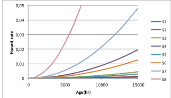
Plotting the failure rate function based on the data and using the equation 12 , in Table 2 , shows that the failure rate function could be approximately of bathtub shape in the 3rd phases mean wear out or deterioration phase.

As it is clear when the system condition is in state 4 , 6, 7, 8 when we have two or three covariate in bad condition the rate of failure is very high and the worst case is state 8 which three covariate are in bad condition (Figure 3).

Fig. 3 Hazard rate function plot based on different covariate state

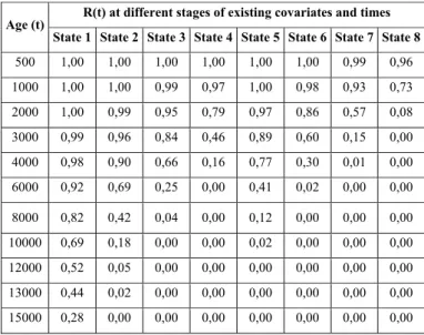
Table 3 represents the value of reliability function considering the effect of different covariates for different operating time. As it is seen the reliability decreases with the both increment of operating time (age) and number of negative influencing covariates. For instance at the age of 3000 (hrs) the reliability at the stage 1 which represents no negative covariates (good condition) is 99% whereas in the states 4 and 7 the reliability values decreases to 46% and 15% respectively where there are two negative influencing factors. (11)

TABLE 2HAZARD RATE FUNCTIONλ(t)FOR WEIBULL PHM CALCULATED FOR DIFFERENT STATES OF COVARIATES

Age (t) λ(t) at different stages of existing covariates and times

State 1 State 2 State 3 State 4 State 5 State 6 State 7 State 8

100 1,13217E-08 5,07403E-08 1,938E-07 8,685E-07 1,248E-07 5,593E-07 2,136E-06 9,573E-06 500 2,83042E-07 1,26851E-06 4,844E-06 2,171E-05 3,12E-06 1,398E-05 5,34E-05 0,0002393 1000 1,13217E-06 5,07403E-06 1,938E-05 8,685E-05 1,248E-05 5,593E-05 0,0002136 0,0009573 2000 4,52868E-06 2,02961E-05 7,751E-05 0,0003474 4,992E-05 0,0002237 0,0008544 0,0038293 3000 1,01895E-05 4,56663E-05 0,0001744 0,0007816 0,0001123 0,0005034 0,0019225 0,0086159 4000 1,81147E-05 8,11845E-05 0,00031 0,0013895 0,0001997 0,0008949 0,0034177 0,0153171 6000 4,07581E-05 0,000182665 0,0006976 0,0031265 0,0004493 0,0020135 0,0076898 0,0344634 8000 7,24588E-05 0,000324738 0,0012402 0,0055581 0,0007987 0,0035796 0,0136708 0,0612683 10000 0,000113217 0,000507403 0,0019378 0,0086846 0,001248 0,0055932 0,0213606 0,0957318 12000 0,000163032 0,00073066 0,0027904 0,0125058 0,0017971 0,0080542 0,0307593 0,1378538 13000 0,000191337 0,000857511 0,0032749 0,014677 0,0021091 0,0094525 0,0360995 0,1617867 15000 0,000254738 0,001141657 0,00436 0,0195403 0,002808 0,0125847 0,0480615 0,2153965

Figure 4 shows the reliability function values for different ages. It is obvious how the existence and state of covariates strongly affects the shape of reliability function.

Fig. 4 Reliability for Weibull PHM calculated in different states of covariates TABLE 3RELIABILITY FUNCTION R(T) FOR WEIBULL PHM CALCULATED

FOR DIFFERENT STATES OF COVARIATES

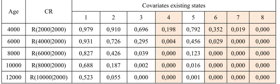
Table 4 similar to Table 3 was obtained for any initial survival time and state of covariates. Table 4 shows the conditional reliability function values calculated for a given initial survival time (current working age) of 2000 (hrs) and different states of influencing parameters.

The conditional reliability function R (t|2000, Z(x) = i) = P (T >x | T > 2000, Z(x) = i) for i = 1, 2, 3, 4, 5, 6 and x > 2000 is illustrated in Figure 5. It is obvious how the state of the covariates strongly affects the shape and value of the conditional reliability function. The situations are worst at the states 4 and 6, 7, 8 when at least two covariate negatively affect the reliability (highlighted column in Table 4).

Fig. 5 Conditional reliability function for Weibull PHM calculated for initial survival time of 2000 (hrs.) and different states of covariates

The MRL for some survival times and different states of existing covariates are presented in Table 5. It should be noted that with an increase of the intense of covariates the expected useful life decreases.

The category eight of existing covariates in Table 5, where all covariates are in the worse condition (with negative impact), indicates the most harmful and unpractical situation.

Age (t) R(t) at different stages of existing covariates and times

State 1 State 2 State 3 State 4 State 5 State 6 State 7 State 8

500 1,00 1,00 1,00 1,00 1,00 1,00 0,99 0,96 1000 1,00 1,00 0,99 0,97 1,00 0,98 0,93 0,73 2000 1,00 0,99 0,95 0,79 0,97 0,86 0,57 0,08 3000 0,99 0,96 0,84 0,46 0,89 0,60 0,15 0,00 4000 0,98 0,90 0,66 0,16 0,77 0,30 0,01 0,00 6000 0,92 0,69 0,25 0,00 0,41 0,02 0,00 0,00 8000 0,82 0,42 0,04 0,00 0,12 0,00 0,00 0,00 10000 0,69 0,18 0,00 0,00 0,02 0,00 0,00 0,00 12000 0,52 0,05 0,00 0,00 0,00 0,00 0,00 0,00 13000 0,44 0,02 0,00 0,00 0,00 0,00 0,00 0,00 15000 0,28 0,00 0,00 0,00 0,00 0,00 0,00 0,00

TABLE 4CONDITIONAL RELIABILITY FUNCTION OR MRL FOR WEIBULL PHM CALCULATED FOR INITIAL SURVIVAL TIME OF 2000(HRS)

AND DIFFERENT STATES OF COVARIATES

TABLE 5MRL(HRS.) FOR WEIBULL PHM CALCULATED INITIAL SURVIVAL TIME T AND DIFFERENT STATES OF COVARIATES

Age Covariates existing states

1 2 3 4 5 6 7 8 1000 11361,24 6506,27 3821,50 1971,51 4572,32 2417,31 1257,94 522,51 2000 10389,79 5576,56 2969,94 1281,85 3689,59 1670,67 704,22 220,30 3000 9460,46 4740,48 2145,93 839,59 2947,04 1152,50 413,59 1943,23 4000 8585,84 4011,42 1759,75 566,62 2348,23 810,11 236,94 … 6000 7025,96 2867,39 1073,12 131,23 1511,32 429,89 … …

It’s a risk alarm for operation in practice and therefore, it’s attempted to avoid that circumstance. Meanwhile, as the MRL in this category for long time operation is unreliable and unrealistic, therefore we ignore to estimate and use the MRL for such condition.

In Figure 6, the MRL function is shown as a function of current working age and the state of covariates at that working age, i.e. the functions e(t, i ) = E(T − t|T > t, Z(t) = i ), for i = 1, 2, 3, 4, 5 and t= 1000, 2000, 3000, 4000 and 6000 (hrs) are shown.

Fig. 6 Remaining expected useful life for Weibull PHM calculated for different initial survival time t and different states of covariates

As it’s obvious in Figure 6, the remaining useful life increases at the state of the covariate 5, where there is only one covariate with negative influence and two with positive. In general, however, the remaining useful life of hydraulic jack decreases as the state of the covariates getting worse, which cause the reliability of system decline.

The remaining useful life of hydraulic jack launched in LHD can be roughly estimated by using the above mentioned graph for rapid evaluation of existing situation. This is an important issue and aspect for infield engineers to make decision on running the project and production.

IV. CONCLUSIONS

The main objective of this study is MRL estimation of hydraulic jack unit of LHD machine in a Swedish mine. Theoretical methods for the calculation of the conditional reliability and MRL given the current age and history of the data were considered. A Weibull PHM with time-independent covariates was used to describe the failure characteristics of the hydraulic jack on LHD machines. The results represent a considerable difference between various operational and environmental condition. So that, as the influence of covariates is getting worse, the remaining useful life shows a decreasing trend. For instance the reliability of the system in the best condition when the covariates are in good (improved) condition decreases slightly, while in bad situation when the covariates are in the worse condition decreases to zero sharply. Also the effect of covariate in MRL is inevitable so that in the good condition the hydraulic jack is expected to work longer than while in worse state. Presented results can be used, for planning of preventive maintenance based on the conditional probability of failure or MRL. In future a more focus will be on the context based MRL estimation where more influencing parameters be considered to achieve more realistic approach and results.

Age CR Covariates existing states

1 2 3 4 5 6 7 8 4000 R(2000|2000) 0,979 0,910 0,696 0,198 0,792 0,352 0,019 0,000 6000 R(4000|2000) 0,931 0,726 0,295 0,004 0,456 0,029 0,000 0,000 8000 R(6000|2000) 0,827 0,426 0,039 0,000 0,123 0,000 0,000 0,000 10000 R(8000|2000) 0,688 0,187 0,002 0,000 0,016 0,000 0,000 0,000 12000 R(10000|2000) 0,523 0,055 0,000 0,000 0,001 0,000 0,000 0,000

ACKNOWLEDGMENT

The authors would like to thank for the support of CAMM (Centre of Advanced Mining & Metallurgy) project in this research work.

REFERENCES

[1] H. E. Ascher and H. Feingold, Repairable System Reliability: Modeling,

Inference, Misconceptions and Their Causes, Marcel Dekker, New

York, 1984

[2] D. Banjevic and A.K.S. Jardine, “Calculation of reliability function and remaining useful life for a Markov failure time process”, IMA Journal

of Management Mathematics, Vol. 17, pp. 115−130, 2006

[3] A. Barabadi, J. Barabady and T. Markeset, “Maintainability analysis considering time-dependent and time-independent covariates

Reliability engineering and System Safety, Vol. 96, No. 1, pp. 210-217,

2011

[4] S. Bimal, B. Sarkar and S. Mukherjee, “Reliability analysis of Shovel Machines Used in an Open Cast Coal Mine”, Journal of Mineral

Resources Engineering, 219-231, 2001

[5] D.R. Cox, “Regression models and life-tables”, Journal of the Royal

Statistical Society, Vol. B34, pp. 187-220, 1972

[6] M. El-Koujok, R. Gouriveau and N. Zerhouni, “From monitoring data to remaining useful life: an evolving approach including uncertainty”, in proceeding 34th _{European Safety Reliability & Data Association,}

SReDA Seminar and 2nd Joint ESReDA/ESRA Seminar, 2008, San

Sebastian, Spain

[7] E. A. Elsayed, Mean residual life and optimal operating conditions for

industrial furnace tubes, Case Studies in Reliability and Maintenance

(W. R. Blischke & D. N. P. Murthy eds), New York, Wiley, pp. 497– 515, 2003

[8] A.H. Elwany and N.Z. Gebraeel, Sensor-driven prognostic models for

equipment replacement and spare parts inventory, IIE Transactions,

Vol. 40, pp. 629–639, 2008

[9] B. Ghodrati, “Reliability and Operating Environment Based Spare Parts Planning”, PhD thesis, Luleå University of Technology, Sweden, 2005

[10] B. Ghodrati and U. Kumar, “Reliability and Operating Environment Based Spare Parts Estimation Approach – A Case Study in Kiruna Mine”, Journal of Quality in Maintenance Engineering, Vol. 11, pp. 168-184, 2005

[11] A.K.S. Jardine, D. Lin and D. Banjevic, “A review on machinery diagnostics and prognostics implementing condition-based maintenance”, Mechanical Systems and Signal Processing, Vol. 20, 1483–1510; 2006

[12] J.D. Kalbfleisch and R.L. Prentice, The Statistical Analysis of Failure

Time Data, New York: John Wiley & Sons, 1980

[13] D. Kumar and B. Klefsjö, “Proportional hazards model: an application to power supply cables of electric mine loaders”, International Journal

of Reliability, Quality and Safety Engineering, Vol. 1, No. 3, pp.

337-352, 1994

[14] U. Kumar, B. Klefsjö and S. Granholm, “Reliability investigation for a fleet of load-haul-dump machines in a Swedish mine”, Reliability

Engineering & System Safety, 26(4):341-361, 1989

[15] U. Kumar, B. Klefsjö, “Reliability analysis of hydraulic systems of LHD machines using the power law process model”, Reliability

Engineering & System Safety, 35(3):217-224, 1992

[16] U. Kumar, Y. Huang, “Reliability analysis of a mine production system: a case study”, Annual Reliability and Maintainability Symposium: Atlanta, Georgia, NJ : IEEE. pp. 167-172, 1993

[17] D. Kumar, J. Crocker, J. Knezevic and M. El-Haram, Reliability,

Maintenance and Logistic Support: a Life Cycle Approach, USA:

Kluwer Academic Publishers, 2000

[18] Sh. Yan, “Reliability modeling and analysis with mean residual life”, Doctoral thesis, National university of Singapore, 2009

[19] L. Wang, J. Chu and W. Mao, “A Condition-Based Replacement And Spare Provisioning Policy For Deteriorating Systems With Uncertain Deterioration To Failure”, European Journal of Operational Research, Vol. 194, 184–205, 2009