Frihamnsstaden

Algorithms for Pure Categorical Optimization

Examensarbete för kandidatexamen i matematik vid Göteborgs universitet

Kandidatarbete inom civilingenjörsutbildningen vid Chalmers tekniska högskola

Oskar Eklund

David Ericsson

Astrid Liljenberg

Adam Östberg

Department of Mathematical Sciences

CHALMERS UNIVERSITY OF TECHNOLOGY

UNIVERSITY OF GOTHENBURG

Algorithms for Pure Categorical Optimization

Examensarbete för kandidatexamen i tillämpad matematik

inom matematikprogrammet vid Göteborgs universitet

Oskar Eklund

David Ericsson

Adam Östberg

Kandidatarbete i matematik inom civilingenjörsprogrammet Teknisk matematik

vid Chalmers tekniska högskola

Astrid Liljenberg

Supervisor: Zuzana Nedělková

Examiners: Marina Axelson-Fisk and Maria Roginskaya

Department of Mathematical Sciences

CHALMERS UNIVERSITY OF TECHNOLOGY

UNIVERSITY OF GOTHENBURG

Preface

Each group member kept an individual time log during the project. We also kept a group log with notes from our group meetings and the meetings with our supervisor.

Work process

During the project we have had group meetings approximately twice per week, as well as mee-tings with our supervisor every 1-2 weeks. During the group meemee-tings we decided on tasks to be done until the next meeting, and followed up and gave feedback on work done since the last meeting. All group members have been involved in and kept up to date on all parts of the project du-ring the process, but we did also assign main areas of responsibility for each group member. Oskar was responsible for the report, David was responsible for the theory and literature studies, Astrid was assigned the role of project coordinator, and Adam was responsible for the Matlab code. During the work process, David has lead the literature studies. Oskar did much of the work on and wrote the code for the global search algorithm. Astrid did everything related to the genetic algorithm, including coding the algorithm. The numerical results were generated by Adam, who also wrote the code for the local search algorithm as well as the code used for benchmarking. All group members contributed with literature studies and creative input when developing the neighborhoods and algorithms. The discussion and conclusion parts of the report are the results of group discussions. All important decisions were discussed and made during group meetings.

Report

The writing of different sections of the report was divided between the group members. The authors of each section are presented below, however, everyone has contributed with ideas, comments, and proofreading of each section.

• Oskar Eklund: 3.1 Previous research, 3.2 Local Search, 3.3 Global Search, 4.1 Test problems, 5.2 Global Search Algorithm

• David Ericsson: 2 Mathematical optimization, 4.2 Benchmarking, 6 Results

• Astrid Liljenberg: Abstract, 1.4 Outline, 3.4 Genetic algorithm, 5.3 Genetic algorithm • Adam Östberg: 4 Assessment methodology, 5.1 Local search algorithm, 5.2 Global search

algorithm, 5.4 Benchmarking, 6 Results

The remaining sections, not mentioned above, were co-authored during group sessions.

Acknowledgements

We would like to thank our supervisor Zuzana Nedělková for the great guidance and insightful advice she has provided us during the course of the project.

Populärvetenskaplig sammanfattning

Optimering handlar om att försöka finna bästa möjliga lösning på ett problem. Inom matematisk optimering innebär detta att man har en funktion, som beroende på de val man gör i problemet, ger ett värde. Det är detta värde man antingen vill minimera eller maximera. Man kan även sätta upp villkor för hur en lösning får lov att se ut. Ett känt exempel på ett optimeringsproblem är kappsäcksproblemet. En person har då en kappsäck och ett urval av föremål att fylla kappsäcken med. Varje föremål har ett värde, men kappsäcken har en begränsat utrymme som gör det omöjligt att packa ner samtliga föremål. Problemet är alltså att bestämma vilka föremål personen ska packa ner i kappsäcken för att den ska få så stort värde som möjligt. I detta exempel utgörs funktionen av det sammanlagda värdet av föremålen i kappsäcken, vilket ska maximeras, och villkoren utgörs av kappsäckens utformning och volym.

Att lösa optimeringsproblem är av stort intresse för samhället, då vi har en begränsad mängd re-surser som vi vill använda på ett effektivt sätt. Av denna anledning har det under lång tid bedrivits forskning inom ämnet optimering. I dagens datoriserade samhälle handlar denna forskning ofta om att utveckla algoritmer, som med hjälp av datorer kan lösa olika problem. I de flesta matematiska optimeringsproblem utgörs valen som funktionen beror på, de så kallade beslutsvariablerna, av tal. Dessa tal har en naturlig ordning vilket innebär att det för varje par av tal är möjligt att jämföra dem och säga att det ena är större än, lika med, eller mindre än det andra. För denna typ av problem finns det många kända algoritmer som används för att hitta lösningar. Men det är inte alltid fallet att variablerna är tal, exempelvis om målet är att maximera värdet av ett hus genom att måla om det i en populär färg. Då handlar det istället om färger, vilka saknar en naturlig ordning eftersom det inte finns ett självklart sätt att avgöra om till exempel röd är större än grön. Detta är vad kategorisk optimering handlar om; att lösa optimeringsproblem med variabler som inte har någon naturlig ordning.

Volvo GTT bedrev åren 2012-2017 ett forskningsprojekt vid namn TyreOpt som behandlade op-timeringsproblemet att välja däck till lastbilar i syfte att minimera bränsleförbrukningen. Detta optimeringsproblem är kategoriskt eftersom däck, likt färger, inte har någon naturlig ordning. Att ett stort företag som Volvo investerar i ett sådant projekt är en god indikation på att kategoriska optimeringsproblem är värda att studera. Vi har därför ägnat vårt arbete till kategorisk optimering, där vi har studerat befintliga algoritmer och även med hjälp av dessa utvecklat egna algoritmer för den här typen av problem.

Vårt arbete har kretsat kring tre algoritmer: en lokalsökningsalgoritm, en globalsökningsalgoritm, och en genetisk algoritm. Lokalsökningsalgoritmen letar inte nödvändigtvis efter den optimala lösningen, utan nöjer sig med att hitta en lösning som är bättre än alla andra lösningar i dess lokala omgivning. Omgivningar kan definieras på olika sätt, i problemet med husfärgerna skulle en omgivning till färgen röd exempelvis kunna inkludera färgerna rosa och orange, eftersom de i någon mening ligger nära färgen röd. Globalsökningsalgoritmen, som vi har utvecklat baserat på lokalsökningsalgoritmen, söker å andra sidan efter den verkligt optimala lösningen av problemet. Både lokal- och globalsökningsalgoritmen kräver en omgivningsdefintion för att användas, något som vi också har studerat i detta arbetet. Slutligen så är den genetiska algoritmen en algoritm inspirerad av den biologiska evolutionen, med mekanismer som till exempel naturligt urval och genmutation. Vi har implementerat alla tre algoritmerna i programmeringsspråket Matlab. Vidare har vi valt ut lämpliga problem att testa algoritmerna på, för att på så sätt kunna analy-sera hur bra de presterar. Vi har använt oss av ett påhittat, rent matematiskt problem, och ett fysikaliskt problem som involverar en balk. Genom att testa hur bra algoritmerna löser problemen har vi kunnat dra slutsatser om hur de kan användas i fortsättningen. Exempelvis har vi sett att lokalsökningsalgoritmen med avseende på en viss omgivningsdefinition, som vi kallar kategorisk om-givning, fungerade väldigt bra i jämförelse med den genetiska algoritmen. Vi har även sett att med en annan omgivningsdefinition, som vi kallar diskret omgivning, fungerar globalsökningsalgoritmen bättre än lokalsökningsalgoritmen. En nackdel vi har kunnat se med globalsökningsalgoritmen är att den i vissa fall tar förhållandevis lång tid för datorn att utföra.

Abstract

Optimization problems with categorical variables are common for example in the automotive industry and other industries where mechanical components are to be selected and combined in favorable ways. The lack of a natural ordering of the decision variables makes categorical op-timization problems generally more difficult to solve than the discrete or continuous problems. Thus it is important to develop methods for solving categorical optimization problems. This report presents three different algorithms that can be used for solving categorical optimiza-tion problems: a local search algorithm, a global search algorithm, and a genetic algorithm. In addition, two different neighborhood definitions to use with the local search algorithm are presented, a categorical one, and a discrete one. The algorithms were implemented in Matlab and were tested on two different categorical optimization problems: an artificial problem, and a beam problem. The algorithms developed were applied to a large number of instances of the problems and their performance was evaluated using performance profiles and data pro-files. The local search algorithm equipped with the categorical neighborhood outperformed the other algorithms considered.

Sammanfattning

Optimeringsproblem med kategoriska variabler är vanligt förekommande exempelvis inom bil-industrin och andra industrier där mekaniska komponenter ska väljas ut och kombineras på gynnsamma sätt. Avsaknaden av naturlig ordning på beslutsvariablerna gör att kategoriska optimeringsproblem oftast är svårare att lösa än diskreta eller kontinuerliga problem. Det är därför viktigt att ta fram metoder som löser kategoriska optimeringsproblem. Den här rapporten presenterar tre olika algoritmer som kan användas för att lösa kategoriska optime-ringsproblem: en lokalsökningsalgoritm, en globalsökningsalgoritm, och en genetisk algoritm. Dessutom presenteras två olika omgivningsdefintioner att använda ihop med lokalsökningsal-goritmen, en diskret, och en kategorisk. Algoritmerna implementerades i Matlab och testades på två olika kategoriska optimeringsproblem: ett artificiellt problem, och ett balkproblem. De framtagna algoritmerna applicerades på ett stort antal instanser av testproblemen och deras prestanda utvärderades med hjälp av prestandaprofiler och dataprofiler. Lokalsökningsalgorit-men utrustad med den kategoriska omgivningen presterade bäst av de testade algoritmerna.

Contents

1 Introduction 1

1.1 Background . . . 1

1.2 Purpose and aim . . . 1

1.3 Scope . . . 1

1.4 Outline . . . 2

2 Mathematical optimization 2 2.1 Overview . . . 2

2.2 Optimization with discrete and categorical variables . . . 3

3 Algorithms for categorical optimization problems 5 3.1 Previous research . . . 5 3.2 Local search . . . 5 3.3 Global search . . . 6 3.4 Genetic algorithm . . . 7 4 Assessment methodology 9 4.1 Test problems . . . 9 4.2 Benchmarking of algorithms . . . 10 5 _{Implementation in Matlab} 11 5.1 Local search algorithm . . . 11

5.2 Global search algorithm . . . 12

5.3 Genetic algorithm . . . 12 5.4 Benchmarking . . . 13 6 Results 14 7 Discussion 17 7.1 Algorithms . . . 17 7.2 TyreOpt . . . 18 8 Conclusion 18 A Photos of tires 20 B Matlab code 21 B.1 Neighborhoods . . . 21 B.1.1 Categorical . . . 21 B.1.2 Discrete . . . 21 B.2 Local search . . . 25 B.2.1 Artificial problem . . . 25 B.2.2 Beam problem . . . 25 B.3 Global search . . . 26 B.3.1 Artificial Problem . . . 26 B.3.2 Beam Problem . . . 27 B.4 Genetic algorithm . . . 29 B.4.1 Artificial problem . . . 29 B.4.2 Beam problem . . . 31 C Summary in Swedish 35 C.1 Inledning . . . 35 C.2 Optimeringslära . . . 35 C.3 Kategorisk optimering . . . 35

1

Introduction

The field of optimization is concerned with finding the best solution to a given problem. The problems are modelled using mathematical tools and can be divided into different branches based on the domain of their decision variables, for example, continuous, and discrete optimization prob-lems. Some discrete optimization problems have variables that lack natural order, that is, there is no meaningful way to order them that corresponds to a physical meaning. Such discrete variables are referred to as categorical variables. Optimization problems having only categorical variables arise in various real life applications and are called pure categorical problems, e.g., an optimization problem to select components in a mechanical construction, see [1].

The existing optimization methods developed for solving problems with continuous or discrete variables cannot be used to solve the categorical optimization problems. This is due to the fact that the usual definitions, for instance neighborhood, optimality, and continuity are not applicable in the context of categorical variables with no natural ordering. In order to analyze and solve pure categorical problems, alternative definitions and solution methods have to be introduced.

1.1

Background

This project was motivated by the research project TyreOpt ([2]) conducted by Chalmers Uni-versity of Technology and UniUni-versity of Gothenburg in cooperation with Volvo Group Trucks Technology (GTT). The main aim of the research project was to reduce the fuel consumption of heavy duty trucks by optimizing the tire selection. The choice of tires for each axle of the truck, that is, discrete variables with no natural ordering, were the categorical decision variables of the tires selection problem.

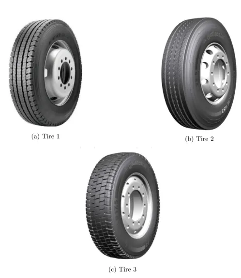
Optimization methods and vehicle dynamics models to select the tires when described by their inflation pressure, diameter, and width were developed in [2]. A possible way to improve the methodology developed is to somehow also consider the tire patterns when selecting the tires. Photos of tires are supplied by Volvo GTT, which can be found in Appendix A, with the purpose to find suitable parameterizations of the tire tread patterns allowing for the tire patterns to be considered as additional variables of the tire selection problem.

1.2

Purpose and aim

The purpose of this bachelor project is to analyze categorical optimization problems and to study and develop algorithms to solve such problems. In particular, the aim is to assess how distance and neighborhoods can be defined for categorical variables, and given suitable definitions of these notions, how a categorical optimization problem can be solved efficiently. In order to do this, several definitions of distance and neighborhood for categorical variables are explored with the intention to develop algorithms solving specific categorical optimization problems. The algorithms are developed utilizing existing approaches from the literature studied and our own ideas. In addition, they are implemented in Matlab and their performance are assessed on different test problems.

1.3

Scope

The project is restricted to the study of pure categorical problems, not considering mixed variable programs (MVP) where the variables may be of both the continuous and discrete (categorical) type. In the theoretical part of the project where we discuss distances and neighborhoods, we do not intend to come up with a completely new definition, but rather review current ones and possibly modify them. We further restrict our project to analyzing three algorithms, called local search, global search and genetic algorithm. For the implementation we restrict the work to two different types of test problems, called the beam problem and the artificial problem, for testing the performance of the three algorithms. In addition, no ethical aspects connected to project that would require further analysis have been identified and will therefore not be discussed in the report.

1.4

Outline

In Section 2 we begin with an introduction to mathematical optimization, defining the concepts of both the local and the global optimum. The optimization problems with categorical variables are subsequently introduced and it is explained how they differ from the optimization problems with discrete or continuous variables. Then, distances and neighborhoods for categorical variables are discussed.

Section 3 introduces the three algorithms developed for solving optimization problems with categor-ical variables, including a local search algorithm for finding local optima, a global search algorithm with the intention to find global optima, as well as a genetic algorithm.

In Section 4 two categorical optimization problems are presented, an artificial, and a real world optimization problem. It is also described how the so-called data and performance profiles can be used to assess the performance of the algorithms. In Section 5 we describe how the algorithms were implemented in Matlab.

The results of numerical tests of the algorithms when applied to the test problems are presented in Section 6, and discussed in Section 7, as well as the implications for the TyreOpt research project. In Section 8 we draw conclusions regarding the algorithms developed for solving optimization problems with categorical variables. Also, we draw conclusions about the TyreOpt project.

2

Mathematical optimization

Mathematical optimization is the discipline concerned with finding the best solution to a given problem. To achieve this, a mathematical model of the problem is set up, and using mathematical methods an optimal solution is searched for. To facilitate the understanding of the technicalities of the report, this section begins by introducing relevant concepts in optimization on a general level. Then, a more detailed account of categorical optimization is given.

2.1

Overview

We begin by setting up the mathematical environment for general optimization problems. In order to describe the choices that can be made in the problem, a space of decision variables Y is introduced. Each element y ∈ Y represents a choice one can make in the problem. To be able to determine which choice is the best, an objective function f : Y → R is needed, which measures how well a decision y ∈ Y solves the problem. In addition, there may be some constraints that need to be satisfied, specifying a subset C of the decision space Y . The set C is often described in terms of constraint functions gi : Y → R satisfying gi(y) = 0 or gi(y) ≤ 0, where i belongs to

some index set I. Equipped with these notions, a general optimization problem may be formulated mathematically as

minimize

y∈Y f (y)

subject to y ∈ C,

(1) where the minimization of the objective function f is taken by convention, since any maximization problem may be converted into a minimization problem by changing the sign of f . We will henceforth use the word optimum and minimum interchangeably. The goal is to find a feasible point, that is, a decision y ∈ Y that fulfills the constraints, i.e., y ∈ C, such that there is no other feasible point with a lower objective value. Such a point is called a global optimum.

Definition 2.1. (Global optimality) A point y ∈ Y ∩ C is said to be a global optimum for the problem (1) if

f (y) ≤ f (x), ∀x ∈ Y ∩ C.

In some problems a global minimum may not exist due to unboundedness of the objective function over the decision space. Even if a global minimum exists, it may be difficult to find it. However, a

point may still have the lowest objective value in a small region around itself. This is the notion of local optimality.

Definition 2.2. (Local optimality) A point y ∈ Y is said to be a local minimum for the problem (1) if

f (y) ≤ f (x), ∀x ∈ N (y) ∩ C, where N (y) is a neighborhood of y.

A neighborhood is a set map N : Y → P(Y ) which assigns to each point y in the decision space a subset of points N (y) ⊂ Y , i.e., N (y) belongs to the power set1 of Y , defining the points in this subset to be similar or close to y. The neighborhood N (y) may be chosen differently depending on the problem, in order to account for what points should be close to each other. For example, when Y ⊆ Rn _{the neighborhood is usually taken as a Euclidean ball, that is, N (y) = {x ∈ Y :}

kx − yk < ε} for some ε > 0. A more thorough discussion of neighborhoods can be found in [3].

2.2

Optimization with discrete and categorical variables

In the previous section general optimization problems were considered, without specifying the underlying decision space nor assumptions on the objective function and the constraints. A discrete optimization problem is a problem in the form (1) with Y ⊆ Zn. Solving discrete optimization problems can easily become cumbersome. Discrete decision spaces can quickly become enormous in size. Consider for example a decision problem with 100 binary variables. For such a problem there are 2100 _{different feasible solutions. The most naive way of solving optimization problems}

is by means of enumeration, that is, computing the objective value for all feasible points in order to check which has the lowest. Such an approach is not appropriate when the decision space becomes enormous. For continuous decision spaces, such as Y ⊆ Rn_{, that are of infinite size,}

tools from calculus have been used to develop algorithms that take shortcuts in order to avoid the enumeration; we refer the reader to [4] for a more in depth description of such algorithms. For discrete cases, development of similar techniques has not been as successful, and the discrete optimization algorithms require much higher effort ([5]).

Categorical optimization problems are ones where the variables represent configurations in some manner. Examples are fixed configuration problems ([6]) and catalog-based design problems ([7]). A fixed configuration problem is when a product with certain components have been decided for, but it remains to choose the dimensions of each component. The catalog-based design problem can be seen as more general, where one chooses components in order to design a tailor-made product. The defining property for such problems is the fact that the decision variables have no natural order. In other words, there is no natural way to compare two elements x and y, as is the case for integers and real numbers.

A categorical optimization problem can be transformed into a discrete one by means of numer-ization as described in [8]. Suppose we have a problem where we need to choose n components, where for the j-th component there are mj possible choices, j = 1, . . . , n. We may then label the

choices for the j-th component by {1, . . . , mj} =: Xj. Hence, the whole set of configurations can

be written as X = X1× · · · × Xn_{, and each configuration can be denoted x = (x}

1, . . . , xn) with

xj ∈ Xj. Thus, a categorical optimization problem may be stated as

minimize

x∈X f (x). (2)

After a numerization, X can be considered a subset of Zn_{. Since the list of configurations can}

be sorted in an arbitrary way, the actual ordering of the choices in the numerization does not necessarily have any real physical meaning. Given all possible orderings of the configurations, one gets a family of discrete problems that all correspond to the same categorical problem.

We now want to define what it means for two configurations x, y ∈ X to be close to each other. However, since it is not certain that the ordering in the discrete problem has some connection to the actual structure of the problem, it makes sense to consider a metric which is invariant under different numerizations. The Hamming distance is such a metric ([8]).

Definition 2.3. (Hamming distance) The Hamming distance between two configurations x, y ∈ X is defined as dH(x, y) = card{i ∈ {1, . . . , n} : xi6= yi}.2

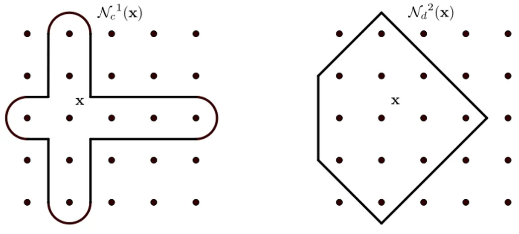
In terms of the Hamming distance, points in the decision space are considered to be close to each other if they differ on few components. With this definition, two points will indeed be close to each other no matter which ordering is chosen in the numerization. Given this metric, a categorical neighborhood may be defined as follows.

Definition 2.4. (Categorical k-neighborhood) Consider the categorical decision space X with the Hamming metric. The categorical k-neighborhood of x ∈ X is defined as Nk

c(x) = {y ∈ X :

dH(x, y) ≤ k}.

Since the categorical problem is defined on Znafter a numerization, one can also consider a discrete neighborhood. This may be appropriate when there is some underlying structure in the ordering of the configurations. An example is the fixed-configuration problem previously mentioned. Definition 2.5. (Discrete t-neighborhood) The discrete t-neighborhood of x ∈ X is defined as Nt

d(x) = {y ∈ X :

Pn

i=1|xi− yi| ≤ t}.

The categorical k-neighborhood contains all configurations such that k components of x may be changed. In the discrete neighborhood, we do not only consider points on the lines parallel to the axes, but points that can be reached in t unit steps. Examples of the categorical 1-neighborhood and the discrete 2-neighborhood are illustrated in Figure 1 and Figure 2 for a categorical space with two decision variables, each having five configurations.

x

Nc1(x)

Figure 1: Categorical neighborhood, k = 1

x

Nd2(x)

Figure 2: Discrete neighborhood, t = 2 Now when the notion of neighborhood for categorical spaces is defined, we can proceed to define optimality conditions. While global optimality for a categorical problem is the same as in the general case, local optimality is defined as follows.

Definition 2.6. (Local optimality with categorical k-neighborhood) A point x ∈ X is said to be a local categorical minimum for the problem (2) if f (x) ≤ f (y) for all y ∈ Nk

c(x).

Definition 2.7. (Local optimality with discrete t-neighborhood) A point x ∈ X is said to be a local discrete minimum for the problem (2) if f (x) ≤ f (y) for all y ∈ N_dt(x).

Local optima are not guaranteed to be global optima. However, many optimization problems of practical relevance exhibit multiple local optima, thus demanding the use of global optimization techniques for their solution. Both local and global optimization techniques for categorical problems are described in Section 3.

3

Algorithms for categorical optimization problems

In this section we commence with an account of the previous research related to our project. Then, three algorithms for solving categorical optimization problems, inspired by the previous research, are laid out. The three algorithms are local search, global search, and genetic algorithm.

3.1

Previous research

Optimization problems with categorical variables can be approached in different ways. One way is discrete optimization algorithms, see for example [9] and [10]. In [9] we find a method for solving discrete optimization problems with help of an auxiliary function. In each iteration this method moves from a local minimum of the objective function to another, better one, with help of the auxiliary function. In [10] a method based on splitting of the set of configurations is presented. For a global descent approach, see [8]. Genetic algorithms have been previously used in many component selection and catalog design problems, see for example [11], [7], and [6]. In our work we utilize the local search algorithm described in [8] and come up with a suggestion for a global search. In [8] a discrete global descent approach of solving categorical optimization problems is used by extending the discrete global descent method described in [9] to categorical problems. There are two suggested extensions: categorical local search and sorting. Categorical local search is also used in our work, and described in the next section. Sorting is a procedure that is based on the fact that different permutations of the variables of a categorical problem lead to categorically equivalent problems. The idea with finding good sortings is to get well-behaved numerical problems which are easy to solve with methods for numerical optimization.

3.2

Local search

The following algorithm for finding local minima of a categorical optimization problem (2) is pre-sented in [8]. This algorithm requires a neighborhood definition and a starting point x0in the set of configurations. We choose the starting point x0_{randomly from the set of feasible configurations.}

The idea of this algorithm is to, in each iteration, loop through the neighborhood of the cur-rent point and search for a point with lower objective value. Let f be the objective function and let N (x) be the neighborhood of a configuration x. The steps of the local search algorithm are presented in Algorithm 1. The algorithm terminates if we for some x, have looped through the neighborhood without having found any y ∈ N (x) \ {x} with f (y) < f∗. That is, if we in one iteration loop through the neighborhood and no configuration in the neighborhood of the current configuration has lower objective value than the current configuration. By having this termination criteria we guarantee that we find a local minimum, according to Definition 2.2. In the worst case scenario we have to compute the objective function for each point in the set of configurations. Algorithm 1 Local Search

1: Choose starting point x = x0and let f∗= f (x).

2: Compute N (x).

3: while Termination criterion is not fulfilled

4: for xi∈ N (x) \ {x}

5: if f (xi) < f∗

6: Let f∗= f (xi_{) and return to Step 2 with x = x}i_.

7: end

8: end

9: end

3.3

Global search

In this section we describe a suggestion for a global search algorithm for categorical optimization problems on the form (2). Although the name suggests this algorithm finds a global minimum, we want to stress that this is an extension of the local search and does not guarantee that a global minimum is found. The extension is focused on finding a good starting point x0, since Algorithm 1 does not provide any computation based suggestions on how to do this. We suggest a procedure on how to select several starting points for Algorithm 1 resulting in a global search algorithm denoted Algorithm 2.

Let us assume that we have the given optimization problem as in (2). As in Algorithm 1, we require a neighborhood defined on X and we also need a set of starting points. Let S ⊂ X be the set of starting points.

The first 6 steps of Algorithm 2 deals with performing local searches with different starting points, where the starting points are suggested to be chosen randomly in X. By doing this we are later able to construct a new starting point which is not randomly chosen. The vector u = (u1, . . . , u|S|) consists of points where ui∈ X is the local optimum returned from Algorithm 1 for i = 1, . . . , |S| and v = (v1, . . . , v|S|) is a vector of objective values where vi = f (ui) for i = 1, . . . , |S|.

In Algorithm 2 we aim to get a better starting point y than the starting points in S in the sense that it is closer to the global optimum of the problem and thus, more often finds lower values. In order to get such a y, we construct a vector of weights w = (w1, . . . , w|S|) in Step 7

of Algorithm 2. To construct w, we need the vector v = (v1, . . . , v|S|) of objective values of the

points in S. We define the index vector a = (a1, . . . , a|S|) by letting aj = |S| for the lowest value

vj of v, ak = |S| − 1 for the second lowest value vk of v and so on up to a` = 1 for the highest

value v` of v. For example, with |S| = 4, if v = (0.13 0.01 1.57 2.31) then a = (3 4 2 1). We then

compute w as wi = ai P|S| j=1aj , ∀i ∈ {1, . . . , |S|}. (3)

We observe the following properties of w:

|S|

X

k=1

wk= 1, (4)

wi≥ wj ⇐⇒ vi≤ vj, ∀i, j ∈ {1, . . . , |S|}. (5)

By (5) we can be sure that lower objective values implies higher weights, which is sought since we in our upcoming construction of y want the points in u to be weighted such that a point ui with lower objective value than another point uj has greater impact on y. Equation (4) says that the sum of the weights is equal to 1, and thus it makes sense to refer to them as weights. When we have computed a weight vector w which satisfies these conditions we are able to construct y in Step 8 of the algorithm. Let N be the number of elements in a configuration x ∈ X. Initially we construct y as yi:= |S| X k=1 wkuik, ∀i ∈ {1, . . . , N }. (6)

This construction does not guarantee that y is a feasible configuration. Thus if needed, we finish this construction by simply rounding y to a feasible configuration to end Step 8. In practice, we do this by letting yi= yirwith

yri := argmin yk∈Xi

(yi− yk), ∀i ∈ {1, . . . , N }. (7)

The motivation behind the construction of y is that we anticipate that it is closer, in the sense of the distance definition given, to the global optimum than just choosing a point randomly out

of X. This is due to the fact that each element yi of y is computed with respect to the objective

values of the outcome of the initial local searches, and in such a way that lower objective value from the initial local search implies stronger impact on yi, for each yi. Further, if y is closer to

the global optimum compared to a starting point randomly chosen out of X, we hope that a lo-cal search from y will result in finding a lower value. However, it is not certain that this is the case. The final step of Algorithm 2 is doing a local search with our constructed y as starting point. Since we can not be sure if f (y∗) < f (ui) ∀i ∈ {1, . . . , |S|}, we return the point with the lowest objective value of y∗ and the points of u.

Algorithm 2 Global Search

1: Choose a set of starting points S ⊂ X.

2: Let v and w be vectors with |S| elements and let u be a vector of points, with |S| elements.

3: for si∈ S

4: Perform Algorithm 1 with starting point x = si.

5: Let ui= x∗ and vi= f (x∗), where x∗ is the point returned from Algorithm 1.

6: end

7: Compute w with respect to u and v as in (2).

8: Compute y ∈ X with respect to u and w as in (5).

9: Perform Algorithm 1 with starting point x = y and let y∗= x∗.

10: Return the point x∗= argmin

u∪{y∗_}

f (x) with objective value f (x∗).

Note that we can not be sure that Algorithm 2 actually finds a better starting point y ∈ X than a randomly chosen starting point in X, since it certainly depends on the structure of the problem. Later sections will show how well Algorithm 2 performs.

3.4

Genetic algorithm

In this section we describe a version of the genetic algorithm presented in [12]. The genetic al-gorithm does not require a neighborhood definition for the problem at hand. This is a difference compared to previous algorithms, and makes it an interesting alternative approach to solving a categorical optimization problem. It is however important to note that there is no way of knowing how good a solution will be found, not even a local optimum is guaranteed. In that sense the genetic algorithm is more of a heuristic, and is usually only used when classical methods cannot be utilized. Another drawback of the genetic algorithm is that there are a lot of parameter values that can be varied. The best values varies between problems, making it difficult to know in advance what parameter values to choose.

The genetic algorithm encodes a set of points or configurations xj ∈ X, j = 1, . . . , N in the search space as a set of chromosomes cj, j = 1, . . . , N , called a population P of size N . It is important that there is one-to-one correspondence between xj and cj, so that a chromosome can be decoded to find the original configuration or point. Chromosomes are also referred to as indi-viduals. The chromosomes are strings of real or integer values, to which a number of biologically inspired operators are applied to form a new population. Each value of a chromosome is called a gene. There are different variations of the genetic algorithm depending on what operators and variations thereof that are chosen during the implementation. One version of the algorithm will be introduced below, followed by detailed descriptions of the different steps, and it is based largely on the book on stochastic optimization by Wahde ([12]).

Algorithm 3 Genetic algorithm

1: Initialize a population P of size N by randomizing chromosomes cj, j = 1, . . . , N .

2: while Termination criterion is not fulfilled. 3: for cj _{∈ P}

4: Using the encoding scheme, decode chromosome cj _{to form configuration x}j _{∈ X.}

5: Evaluate f (xj_{), where f is the objective function.}

6: Based on the objective value, assign a fitness value Fj _{to the individual.}

7: end

8: Let Pnew := ∅ be an empty set of chromosomes.

9: for j = 1, . . .N₂

10: Select with replacement two individuals i1 and i2 from P using the selection operator.

11: With probability pc, crossover i1 and i2to form new individuals i1new and i 2 new.

12: Perform mutation on i1_new and i2_new.

13: Let Pnew:= Pnew∪ {i1new, i 2 new}.

14: end

15: Replace an arbitrary individual in Pnew with celite∈ P such that Felite≥ Fk, k = 1, . . . , N .

16: Let P := Pnew.

17: end

18: Return the configuration xj ∈ X such that Fj_{≥ F}k_{, k = 1, . . . , N , and objective value f (x}j_).

The first thing to decide on is what encoding scheme to use. The purpose of an encoding is to have a translation between a point, or configuration for categorical problems, and a chromosome. An example is binary encoding, which was first introduced by Holland ([13]). On a one-dimensional continuous problem, the variable x ∈ [−d, d] = X is encoded as a chromosome c = (c1, . . . ck) of

optional length k. Each gene ci is either a 0 or 1, and the corresponding point x is given by

x = −d + 2d

1 − 2−k(2 −1_c

1+ . . . + 2−kck).

Once an encoding scheme is selected, a population of individuals is randomly generated (Step 1) by uniformly randomizing the values of the genes from the permitted interval or set of values. In the case of binary encoding the set would be {0, 1}. Based on this initial population, a new generation will be formed.

In order to decide which individuals will be selected to make up next generation’s population, we need to evaluate the current population (Step 5) and assign a fitness value to each individual (Step 6). To evaluate a chromosome, it must first be decoded using the encoding scheme back-wards (Step 4), and then the corresponding configuration is evaluated in the objective function. A higher fitness value should always correspond to a better solution. For maximization problems the fitness value of an individual is usually taken to be the objective value of the configuration, while minimization problem instead usually uses the multiplicative or additive inverse of the objective value.

Based on the assigned fitness values, individuals of the population should now be selected for reproduction (Step 10). Two common methods of selection are roulette-wheel selection and tour-nament selection. In the former, the probability of selecting an individual is directly proportional its fitness value, while in the latter, individuals are compared and the one with a larger fitness value is assigned a fixed, higher probability regardless of how much larger the fitness value is. The selection operator is then repeatedly applied to the population, each time selecting two indi-viduals i1 and i2 from P . Note that selection is done with replacement, i.e. the same individual may be selected multiple times. To each pair, the crossover operator is applied with some proba-bility pc (Step 11). The point of the crossover is to combine the two individuals to form two new

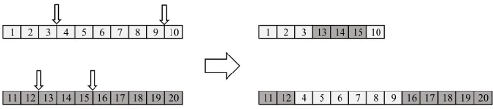
individuals, hopefully corresponding to better solutions to the optimization problem. Usually one or more crossover points are generated and the genes are swapped accordingly, see Figure 3 for an illustration of two point crossover. In the example, the lengths of the chromosomes are not

preserved. If desired, this is fixed by using the same crossover points on both individuals. There is a 1 − pcprobability of no crossover occurring, in which case the new pair of individuals is identical

to the old.

1 2 3 4 5 6 7 8 9 10 1 2 3 13 14 15 10

11 12 13 14 15 16 17 18 19 20 11 12 4 5 6 7 8 9 16 17 18 19 20

Figure 3: An illustration of non length preserving two point crossover. The small arrows indicate the randomly generated crossover points.

Each gene in each chromosome then has a probability pmutof mutating (Step 12). This means that

the gene is replaced with a new value. How the new gene is generated varies, the most common method being to uniformly generate it at random.

Finally, the elitism operator copies the individual with highest fitness value in the current popula-tion and inserts one or a few copies of it into the next generapopula-tion (Step 15). This makes sure that the best individual is never lost, which could otherwise happen due to bad luck during crossover and mutation.

This process of forming new generations is repeated until some termination criterion is met. It could be that a fixed number of generations have been evaluated, or that some convergence cri-terion is fulfilled, for example that the optimal value has not improved for a certain number of generations.

4

Assessment methodology

In order to evaluate the algorithms and different neighborhoods described above, the algorithms will be applied to different test problems. In this section, we first describe the test problems consisting of an artificial optimization problem without any physical interpretation and a beam design optimization problem. Then, performance profiles used to assess how well the algorithms perform will be explained.

4.1

Test problems

The first test problem, referred to as the artificial problem, is to minimize x,z 1 2z T_{Qz + p}T_{z + (diag(z)z)}T_Sz, subject to zi= Zi(xi), i = 1, . . . , m, xi∈ Xi, i = 1, . . . , m, (8)

where Q and S are diagonal matrices with elements Qii ∈ [−3, 3] and Sii ∈ [−3, 3] respectively,

which are uniformly randomly generated. Further, p is a row vector with elements pi ∈ [−1, 1],

which are also uniformly randomly distributed. The set of feasible designs X consists of vectors x ∈ Rmsuch that the number of feasible designs Niin each choice domain Xi is randomized from

the integer uniform distribution on [10, 30] for each i = 1, . . . , m. Further, m is randomized from the integer uniform distribution on [4, 8]. Lastly, Z is a table mapping which is randomly generated such that Zi: Xi→ RNi maps each xi∈ Xionto a vector with Nielements, for each i = 1, . . . , m.

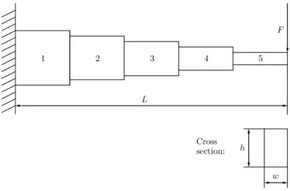
The second test problem stems from an article written by Thanedar and Vanderplaats ([14]), and regards a cantilever beam that is fixed to the wall at its left end and loaded with a constant force F at its right end, see Figure 4. The beam is of length L and consists of K parts, referred to as segments.

Figure 4: Stepped cantilever beam consisting of five segments loaded with a force at its right end Each segment is considered to have two design variables, a height h and a width w. The origi-nal problem in [14] was to minimize the volume of the beam subject to constraints regarding a maximal allowable deflection and the bending stress in each segment. However, in this project we will consider a simplified version, the problem to minimize the deflection of the beam subject to an aspect ratio between the height and the width of each segment, namely h ≤ 30w. We consider the set of all configurations for each segment are combinations of heights and widths chosen from the set of M uniformly spaced points in the interval [450, 600] and [20, 50] respectively. Hence, the distance between the points is fixed and will be the length of the intervals divided by the number of configurations, namely `1 := 150<sub>M</sub> and `2 := 30_M. The beam is modelled by partial differential

equations based on beam theory from Timoshenko and Gere ([15]), which then are solved using the Finite Element Method. A more profound explanation of the modelling can be found in [14]. The problem to be solved is then

minimize x=(x1,...,xK) f (x) subject to xi= (xhi, x w i ) ∈ {(h, w) ∈ R 2_{: (h, w) ∈ X}h_{× X}w_{} i = 1, . . . , K} (9)

where f measures the deflection, and Xh

:= {h ∈ R : h = 450 + k`1, k = 0, . . . , , M } and

Xw

:= {w ∈ R : w = 20+k`2, k = 0, . . . , M } are the sets of the heights and the widths respectively.

4.2

Benchmarking of algorithms

In order to assess and measure the performance of the algorithms we use the techniques introduced by Morà c and Wild ([16]), and Dolan and Morà c ([17]), namely data profiles and performance profiles. Let A be the set of the algorithms. The idea is to gather data by applying each algorithm a ∈ A on a large set of test problems P. In our case the set of test problems consists of an equal amount of instances of the beam problem and the artificial problem, where each problem will be generated with a random number of variables as well as a random number of designs for the variables. For a problem p ∈ P and a algorithm a ∈ A, the performance metric tp,a, defined as the

number of function evaluations required to satisfy a convergence test, will be used to construct the profiles. The following convergence test, suggested by Morà c and Wild ([16]), is used; a feasible design z satisfies the convergence test if

f (z0) − f (z) ≥ (1 − τ )(f (z0) − fmin). (10)

Here z0 _{is the starting point for the problem, f}

min is computed for each problem as the

small-est objective value found using any of the algorithms, and τ ∈ [0, 1] is the tolerance parameter representing the desired decrease from the starting objective value f (z0_{). Hence, the algorithm is}

said to converge at the feasible point z if the reduction f (z0_{) − f (z) is at least (1 − τ ) times the}

reduction f (z0) − fmin. By convention, if the algorithm a fails to satisfy the convergence test for

problem p, then tp,a= ∞.

The performance profile, originally introduced by Dolan and Morà c ([17]), is obtained from the performance metric by computing the the performance ratio, that is for problem p and algortihm a

rp,a=

tp,a

min{tp,a: a ∈ A}

. The performance profile for algorithm a is then defined as

ρa(α) =

1

|P|size{p ∈ P : rp,a≤ α}. (11)

Thus, the performance profile is the cumulative distribution function for the ratio rp,a. Plotting

these functions for all algorithms provides information about the relative performance of each algo-rithm and the probability for each algoalgo-rithm to satisfy the convergence test. Note that evaluating the function ρa(α) at α = 1 gives the percentage of problems on which algorithm a converges with

the least amount of function evaluations compared to the other algorithms. Additionally, the value of α when the function first attains the value 1, yields that the algorithm never requires more than α times the best algorithm’s number of function evaluations in order to converge. However, the performance profile does not provide sufficient information when the measure of interest is expensive function evaluations, for instance if there is an upper limit on the number function eval-uations allowed. In order to account for this, we use the data profile as additional way to measure performance. The data profile for algorithm a is defined as

da(β) =

1

|P|size{p ∈ P : tp,a≤ β}, (12)

that is, the percentage of problems that satisfy the convergence test in equation (10) within β function evaluations.

Additionally, examples of plots of the objective value against the number of function evaluation will be provided in order to illustrate the trajectory leading to the optimal value found.

5

_{Implementation in Matlab}

In this section a thorough description of how the algorithms, the test problems, and the bench-marking were implemented in Matlab is presented. The implementation was done in Matlab R2015b and carried out on a computer equipped with Intel Core i5 2.7 GHz and 8 GB RAM, running macOS Sierra. The code implementing the algorithms can be found in Appendix B.

5.1

Local search algorithm

The implementation of the local search algorithm was decomposed into two parts; a main file consisting of the basic steps of the algorithm and a function finding the neighborhood. We have chosen to use the categorical 1-neighborhood and the discrete 3-neighborhood. These are

hence-to alter between the discrete and categorical neighborhood without affecting the remaining steps of the algorithm. A description of the Matlab implementation of the main steps of the pseudo code introduced in Section 3.2 follows.

The first step of the local search algorithm, namely choosing a starting point, was made ran-domly generating a uniformly distributed random integer between 1 and the number of feasible designs for each of the variables.

The second step of the algorithm was to find the neighborhood for a given problem and a con-figuration. In opposition to traversing the feasible set and successively add those configurations that satisfies the definition, the neighborhood functions were implemented to construct the set of configurations differing in the given number of elements.

Lastly, the termination criterion was implemented as a boolean variable, keeping track of whether there was a configuration with a lower objective value in the neighborhood or not. Depending on the value of this boolean variable either a new search iteration is performed resulting in a new bet-ter configuration or the local search algorithm (Algorithm 1) bet-terminates and returns the optimal configuration found.

In addition, we created a function in Matlab which returns the optimal point and has the starting point as an input parameter. Also, this function includes a counter, allowing us to keep track of how many function evaluations it takes to reach a minimum. Further, we implemented the local search algorithm with both categorical and discrete neighborhood.

The Matlab code finding the neighborhoods can be found in Appendix B.1 and the Matlab code performing the local search algorithm can be found in Appendix B.2.

5.2

Global search algorithm

The implementation of global search algorithm is partly based on the local search algorithm. In addition to the local search algorithm described in the previous section, the global search algorithm contains two additional steps: computing the weight vector and the new starting point. The global search algorithm was only implemented with the discrete neighborhood and the Matlab code can be found in Appendix B.3.

The size of the starting set was chosen to be three points with the aim to increase the prob-ability of finding a successful local minimum while still limiting the total number of function evaluations until termination. These starting points were chosen randomly from the feasible set. Then, three local searches were performed producing a vector of three local minima. The vector of local minimum is sorted and then each local minimum is assigned its corresponding weight. In order to obtain the new starting point we multiply the weight vector with the vector of local minima. However, it is not assured that this new point is a feasible configuration. Thus, we round this new point according to equation (7). Starting from this new point, we perform a local search yielding a new local minimum. Lastly, we compare the four local minima found and return the one with the lowest objective value.

5.3

Genetic algorithm

The genetic algorithm can be varied in many different ways, and what follows is a description of the operators we used in our implementation of the algorithm. For full Matlab code see Appendix B.4. For our encoding scheme in the artificial problem with m variables a configuration xj_{= (x}j

1, . . . , xjm)

∈ X was encoded as a chromosome cj _{= (c}j 1, . . . , c

j

m) with the genes c j 1 = x j 1, . . . , c j m = xjm.

For the beam problem, a configuration with K beam sections was encoded as a chromosome cj = (cj₁, . . . , cj_2K) with genes cj₁ = xw1, c j 2 = x h 1, . . . , c j 2K−1 = x w K, c j 2K = x h K, where x w k is the

width of beam section k, and xh

are not very efficient for problems with few variables ([12]), but we used it for simplicity. Popu-lation sizes anywhere between 30 and 1000 are common ([12]), but to keep down the number of function evaluations, we used 20 individuals.

Since both the beam problem and the artificial problem are minimization problems, the fitness values of the individuals were assigned as the additive inverse of the objective value. The reason why we did not use multiplicative inverse is that the objective function in the artificial problem may take on negative values. For example, individuals with objective values −2 and 2 would then have been assigned fitness values −1₂ and 1₂ respectively, which does not comply with the conven-tion that better individuals should be assigned higher fitness values.

The best set of parameter values depend on the problem and are not known beforehand. We therefore chose parameters quite arbitrarily within reasonable intervals that usually perform al-right. The tournament selection parameter should be in the interval (0.5, 1), typically around 0.7-0.8 ([12]). We used tournament selection with a tournament size of two randomly selected individuals, of which the one with higher fitness was selected with probability 0.7.

Crossover was applied using one randomly generated crossover point. The same point was used for both individuals since the encoding used in both problems required a fixed chromosome length. The crossover probability can be anywhere in the interval [0, 1] and varies a lot between problems, and we set it to 0.6 in our implementation.

We used two kinds of mutations, regular mutation where a gene is replaced by a randomly gen-erated one, and a variation of the so called creep mutation. We chose for mutation to happen to each gene with probability _m1, where m is the number of genes, since can be shown that a mutation probability somewhere around pmut = _m1 usually works well ([12]). Once it had been

determined that mutation should take place at all the probability of regular mutation was 0.5 and creep mutation 0.5 since we did not know which type of mutation would work best.

Instead of generating the value of new gene randomly, the creep mutation in the beam prob-lem either increased or decreased the value of the gene by the smallest amount allowed, or did nothing to the gene, each with an equal probability of 1₃. In practice this means that a dimen-sion of a beam section would be increased or decreased one step. For the artificial problem creep mutation meant randomizing a new integer within the interval of ±5% of the allowed variable range surrounding the old gene. Looking at values close to the old one could be thought of as fine tuning the solution. However, for the creep mutation to be able to do any fine tuning in the case of a categorical optimization problem, there needs to be an underlying structure to the problem. Without some sort of underlying structure, there would be no reason to believe that a value close the old gene would result in a better solution than a value far away.

One copy of the best individual was inserted into the new generation in the elitism step each iteration, and it always replaced the first individual in the generated population.

5.4

Benchmarking

In order to benchmark the algorithms we used 100 instances of the test problems, 50 beam problems and 50 artificial problems. The beam problems were generated with a random number of segments between 2 and 6 and a random number of feasible designs common for all segments between 10 and 30. The artificial problems were generated according to section 4.1.

The set of algorithms consists of the local search algorithm with categorical neighborhood LS-C, the local search with discrete neighborhood LS-D, the global search with discrete neighborhood GS-D, and the genetic algorithm GA. Hence we have that A = {LS-C, LS-D, GS-D, GA}. Before we applied the algorithms to these problems we computed the convergence criterion, that is the right hand side of inequality (10). That requires a starting point, a known approximate

op-timal solution to the problem and a value of the tolerance parameter τ . To make the performance comparison as fair as possible we let the genetic algorithm generate an initial population and then randomize the starting point for the rest of the algorithms from this population. Further, the best approximate solutions were found in different ways depending on the type of problem. The beam problems have a known optimal solution, namely the maximal height and width of each segment. However, the optimal solutions to the artificial problems are not known. We did empirical tests, comparing the different algorithms, which yielded that the local search with categorical neighbor-hood was the best algorithm to apply the artificial problem in order to get an approximate optimal solution. The tolerance parameter, representing the sought decrease from the starting objective value, was chosen to be τ = 0.1 and τ = 0.01.

Then, equipped with starting points and a convergence criterion, we applied the algorithms to each of the problems and recorded the number of objective function evaluations until the conver-gence criterion was satisfied. If the algorithms failed to satisfy the converconver-gence criterion before terminating, the performance metric was set to infinity. Note that for the genetic algorithm, the maximum number of function evaluation is predetermined by the population size times the number of generations. We set the number of generations to 300 yielding a maximum number of evaluations to 6000. If, however, the genetic algorithm did not converge within this number of function eval-uations the performance metric were set to infinity. This resulted in a matrix with the dimension 100 · |A|. Further, we created the vectors α and β with 100 uniformly spaced points in [1, 40] and [1, 6000] respectively. Then, after using equation (11) and (12) with the acquired matrix and α and β we plot the data profile and the performance profile.

6

Results

This section presents the benchmarking results of the algorithms introduced in Section 3. First, the data and performance profiles will be illustrated alongside some underlying numerical values for the two choices of the tolerance parameter τ . Then, for two specific examples of the beam and artificial problem, an illustration of the objective value against the number of function evaluations is shown.

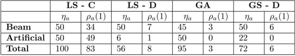
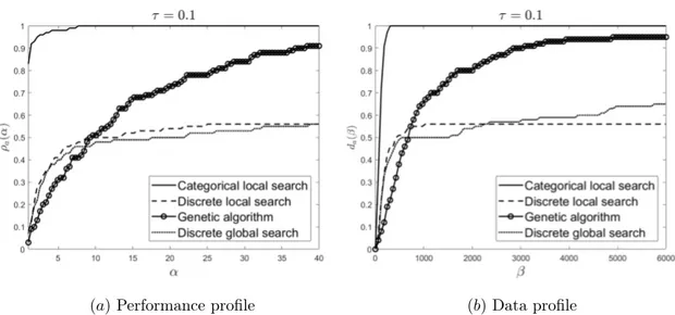
In Figure 5 the performance profile and data profile for the algorithms are shown with tolerance parameter τ = 0.1. The main numerical results are illustrated below in Table 1.

Table 1: The number of problems where the algorithm a ∈ A converges according to (10) with τ = 0.1, ηa = card{p ∈ P : tp,a < ∞}, and the number of problems for which the algorithm

converges in the least amount of function evaluations compared to the other algorithms, ρa(1).

LS - C LS - D GA GS - D

ηa ρa(1) ηa ρa(1) ηa ρa(1) ηa ρa(1)

Beam 50 34 50 7 45 3 50 6

Artificial 50 49 6 1 50 0 22 0

(a) Performance profile (b) Data profile

Figure 5: Data profile da(α) and performance profile ρa(β) for the algorithms applied to 50

in-stances of beam problems and 50 inin-stances of artificial problems with τ = 0.1.

For this randomized set of 50 instances each of the test problems, the categorical local search was the only algorithm that converged in all problem instances. In addition, it converges in the least number of function evaluations in 83% of the problems. In contrast, the genetic algorithm converges for 95% of the problem instances, but only in 3 cases with the least number of function evaluations. The discrete local search converges in all instances of the beam problem, but only in 3 instances of the artificial problem. In comparison, the discrete global search also converges in all instances of the beam problem, however, it converges in 22 cases of the artificial problem. Additionally, since ρa(α) = 1 when α ≥ 8 for the categorical local search algorithm, this algorithm

never requires more than 8 times the number of function evaluations needed for the best performing algorithm.

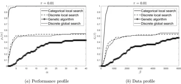
In Figure 6 the performance profile and data profile for the algorithms are shown with the tolerance parameter τ = 0.01. The main numerical results are illustrated below in Table 2.

Table 2: The number of problems where the algorithm a ∈ A converges according to (10) with τ = 0.01, ηa = card{p ∈ P : tp,a < ∞}, and the number of problems for which the algorithm

converges in the fewest function evaluations compared to the other algorithms, ρa(1).

LS - C LS - D GA GS - D

ηa ρa(1) ηa ρa(1) ηa ρa(1) ηa ρa(1)

Beam 50 32 50 13 4 0 50 5

Artificial 50 49 3 1 43 0 8 0

(a) Performance profile (b) Data profile

Figure 6: Data profile da(α) and performance profile ρa(β) for the algorithms applied to 50

in-stances of the beam problems and 50 inin-stances of the artificial problems with τ = 0.01.

With this stricter tolerance parameter, the categorical local search is still the only algorithm that converges in all problem instances. The number of problem instances where it converges in the least number of function evaluation is about the same, this time 81%. Similarly to the case τ = 0.1, both the discrete local search and the discrete global search algorithms converge in all instances of the beam problem. The number of instances of the artificial problem in which they converge is smaller though. Finally, the number of instances where the genetic algorithm converges is reduced by over 50% from 95 to 47, converging only in 4 instances of the beam problem. In addition, it is never the first algorithm to converge. This time we see that for the categorical local search, ρa(α) = 1 for α ≥ 5, hence it never requires more than 5 times the number of function evaluations

needed for the best performing algorithm before it converges.

(a) Beam problem with five segments (b) Artificial problem with five variables Figure 7: Example of a plot of the objective value against the number of function evaluations for all algorithms on the two test problems.

In Figure 7, an example of the algorithms solving an instance of the beam problem (a) and an instance of the artificial problem (b) is shown. The objective value is plotted against the number of function evaluations. In the beam problem, the genetic terminates at 6000 function evaluations and the global search algorithm terminates at 9640 function evaluations. The corresponding numbers of function evaluations for the artificial problem are 6000 for the genetic algorithm and 4541 for the

global search algorithm. However, the graphs are cut at 2000 function evaluations since neither the genetic algorithm nor the global search algorithm descend in any of the problem instances after that. Similarly to the results from the profiles, both the local searches and the global search performs better than the genetic algorithm on the beam problem. In the artificial problem, the local search with categorical neighborhood and the genetic algorithm terminates at the same configuration.

7

Discussion

Initially we will discuss the results of the numerical tests of the different algorithms. Then the possible implications for TyreOpt research project will be laid out.

7.1

Algorithms

The results show that according to the data and performance profiles, the categorical local search algorithm performs the best out of the tested algorithms. We will now discuss the credibility of this result.

Firstly, although we have used a total of 100 different test problems, it may not necessarily be the case that these are representative enough. It could have been valuable if there were more test problems of different character, rather than only two. Secondly, while the choice of fmin for the

beam problems was given since the global optimum was known, it could have been done differently in the case of the artificial problems. In order to find a better approximate optimal solution, one could have let all algorithms solve the problem and take the best one. However, the choice of using the categorical local search was made because it is faster. It could have been interesting to only include test problems with known optimal solutions a priori, in order to see how many times the global optimum was found. However, the convergence test served as an adequate substitute. Although the categorical neighborhood performs better than the discrete one in general, it is worth noting that the discrete local search converged first in 13 instances of the beam problem. Since the beam problem has an underlying structure, it may be beneficent to use a discrete neighborhood in situations where this is the case. As the categorical local search converges first in 49 out of the 50 instances of the artificial problem (see Table 2) with the stricter convergence criterion, the categorical neighborhood seems to be the appropriate choice when there is no underlying structure. The fact that the genetic algorithm took such a downfall when the tolerance parameter was changed from 0.1 to 0.01 to get a stricter convergence criterion is a sign that it manages to find approximate solutions, but not exact and efficient ones, where the latter is measured in number of function eval-uations. Improvements of the genetic algorithm could be made by adjusting the parameter values depending on the problem at hand. Choosing different implementations of the operators, such as roulette-wheel selection or two-point crossover could also possibly improve the performance of the algorithm. Another possible enhancement could be to choose a different encoding scheme that pro-duces longer chromosomes. However, all of these possible improvements are problem dependent, and it is difficult to know beforehand what modifications will improve the algorithm when solving a specific problem.

In the global search algorithm one can think of several ways to improve the algorithm. One example of a way to improve the algorithm is to change how to choose the starting points in S. In our version of the algorithm, we simply chose them randomly out of the set of feasible configurations but with an a priori known underlying structure of the problem the choosing procedure could for example be based on some computations. One thing to compute could be distance between points and it may be a good idea to have a large distance between starting points since we want to minimize the risk that the different local searches make the same function evaluations. If we have a discrete problem a suggestion of a different starting point set would be the corner points, or some of the corner points. The set of corner points Xc_{of a configuration set X, with n elements in each configuration,}

search algorithm could be to change the construction of the new starting point y or having several new starting points instead of one.

It is noteworthy that an algorithm such as the local search yields better results than the ge-netic algorithm, while being very simplistic in nature based on basic optimization theory. Further, there does not exist many algorithms for categorical optimization, and much research has not been done within this topic.

7.2

TyreOpt

The photos of tires provided by Volvo GTT can be found in Appendix A. These photos were supposed to be used to parametrize the tire patterns. When a suitable parametrization is found, the tire tread patterns can be used as additional decision variables in the tires selection problem being solved with TyreOpt. However, in our opinion the supplied photos were not sufficiently well taken. The photographs of the tires were not taken straight from the front but slightly from the side making it complicated to do further numerical analysis. If the photos were taken from the front we suggest three possible parameterizations using image analysis. Firstly, one could define variables based on the percentage of the photo of the tire that consists of groove. Secondly, one could use the number of different directions of the groove patterns. Lastly, one could extract variables based on the direction in which the majority of the grooves were directed. The tread pattern then results in several additional decision variables to be added to the vehicle dynamics models developed within TyreOpt project. For all the parametrizations suggested both the neighborhoods definitions introduced in Section 2 can be used allowing the optimization methodology developed within TyreOpt research project to be applied for the extended tires selection without any further changes.

8

Conclusion

In this project we have implemented three algorithms for solving categorical optimization problems. Two of these algorithms depend on neighborhoods that we have introduced. We have found that with a suitable neighborhood and a relatively simple algorithm, it is possible to outperform genetic algorithms, which have previously been used frequently within categorical problems. In addition, we have improved the local search algorithm by expanding it into a global search algorithm. Nonetheless, we believe that the global search algorithm could become more sophisticated after further development.

With regards to the TyreOpt project, we found that the photos of the tires provided were not sufficiently useful. However, if the photos are taken as we have recommended, the tread pattern can be directly used as an additional set of decision variables in the tire selection problem. For this purpose, we have suggested three parametrizations of the tire treads.

We encourage further use and development of neighborhood-based algorithms in favor of the genetic algorithms, as they provide an opportunity to deepen the understanding of categorical optimization.

References

[1] Carlson SE, Shonkwilerm R, Ingrim E. Comparison of three non-derivative optimization methods with a genetic algorithm for component selection. Journal of Engineering Design. 1994;5(4):367–378.

[2] Nedělková Z. Optimization of truck tyres selection. Chalmers University of Technology. Department of Mathematical Sciences; 2018. PhD thesis.

[3] Rothlauf F. Design of Modern Heuristics: Principles and Application. 1st ed. Springer Publishing Company, Incorporated; 2011.

[4] Andréasson N, Evgrafov A, Patriksson M, Gustavsson E, Nedělková Z, Sou KC, et al. An introduction to continuous optimization. Lund, Sweden: Studentlitteratur; 2016.

[5] Parker RG, Rardin RL. Discrete Optimization. San Diego, CA, USA: Academic Press Pro-fessional, Inc.; 1988.

[6] Brown DR, Hwang KY. Solving fixed configuration problems with genetic search. Research in Engineering Design. 1993;5(2):80–87.

[7] Carlson-Skalak S, White MD, Teng Y. Using an evolutionary algorithm for catalog design. Research in Engineering Design. 1998;10(2):63–83.

[8] Lindroth P, Patriksson M. Pure categorical optimization: a global descent approach. Chalmers University of Technology, University of Gothenburg, Department of Mathematical Sciences; 2011. Technical report.

[9] Ng CK, Li D, Zhang LS. Discrete global descent method for discrete global optimization and nonlinear integer programming. Journal of Global Optimization. 2007;37(3):357–379.

[10] Fuchs M, Neumaier A. Discrete search in design optimization. In: Complex Systems Design & Management. Springer; 2010. p. 113–122.

[11] Carlson SE. Genetic algorithm attributes for component selection. Research in Engineering Design. 1996;8(1):33–51.

[12] Wahde M. Biologically inspired optimization methods: an introduction. Ashurst Lodge, Ashurst, Southampton, UK: WIT press; 2008.

[13] Holland JH. Adaptation in Natural and Artificial Systems. University of Michigan Press; 1975.

[14] Thanedar P, Vanderplaats G. Survey of discrete variable optimization for structural design. Journal of Structural Engineering. 1995;121(2):301–306.

[15] Timoshenko S, Gere JM. Mechanics of Materials. Boston, MA, US: Van Nostrand Reinhold Co.; 1972.

[16] Moré JJ, Wild SM. Benchmarking derivative-free optimization algorithms. SIAM Journal on Optimization. 2009;20(1):172–191.

[17] Dolan ED, Moré JJ. Benchmarking optimization software with performance profiles. Mathe-matical programming. 2002;91(2):201–213.

A

Photos of tires

(a) Tire 1 _{(b) Tire 2}

(c) Tire 3