1876-6102 © 2017 Published by Elsevier Ltd. This is an open access article under the CC BY-NC-ND license (http://creativecommons.org/licenses/by-nc-nd/4.0/).
Peer-review under responsibility of the scientific committee of the 8th International Conference on Applied Energy. doi: 10.1016/j.egypro.2017.03.775
Energy Procedia 105 ( 2017 ) 2684 – 2689
ScienceDirect
* Corresponding author. Tel.: +46-70-791 65 02; E-mail address: anna.frost@mdh.se.
The 8
thInternational Conference on Applied Energy – ICAE2016
Patterns and temporal resolution in commercial and industrial
typical load profiles
Anna E. Frost
a*
, Maher Azaza
a, Hailong Li
aand Fredrik Wallin
aaMälardalen University, Future Energy Center, Box 883, 721 23 Västerås
Abstract
Load patterns often have a periodicity of a day, week and year, which can be taken advantage of when preprocessing load data before clustering. A typical load profile, which reflects the customer's load for a characteristic day, week or year, could be constructed to reduce the data to be processed during the clustering. Typical Daily Profiles (TDP) and Typical Weekly Profiles (TWP) are compared to see how the time resolution of data affects the clustering. Results show that the number of clusters affects the Davies-Bouldin Index and the Dunn Index more than the temporal resolution of data as well as if TDPs or TWPs are clustered. Further, clustering based on customers' TWP instead of TDP makes it easier to find customers which have equipment turned on during Saturdays. This could be of importance when clustering is used to improve forecasting, distribution planning or tariff design.
© 2016 The Authors. Published by Elsevier Ltd.
Selection and/or peer-review under responsibility of ICAE
Keywords: Smart meter; Big data; Load profiles; Clustering; Preprocessing
1. Introduction
With the roll out of more smart meters, more data about consumers' loads are available, which is both an opportunity and a challenge. One of the major challenges with big data in the energy system is how to efficiently mine and analyze the increasing amount of data [1]. One useful method is clustering, which can be used to find data sets with similar patterns or features. Clustering could be applied on massive load data to improve forecasting, distribution planning or tariff design [2]. It could also increase the understanding of the users and find similarities between groups of customers.
Within Big Data it is often spoken about volume, variety, velocity and value (4V) of the data, which also has to be considered when handling data within energy systems [1]. One major issue when clustering load profiles is that the volume of load data easily becomes high. High volume means a high dimensionality of the clustering problem, which makes the algorithm computationally slower. By using a characteristic load profile over a time period, the volume can be limited. A day [3,4] or a week [5] are common periodicity for load patterns and are therefore time periods which can be used to construct a © 2017 Published by Elsevier Ltd. This is an open access article under the CC BY-NC-ND license
(http://creativecommons.org/licenses/by-nc-nd/4.0/).
typical load profile (TLP) [6]. These can be called Typical Daily Profile (TDP) [3] or Typical Weekly Profile (TWP), depending on the chosen time period.
Chicco [7] suggested a four step load pattern categorization procedure: i) Data gathering and processing, ii) pre-clustering phase, iii) clustering phase and iv) post-clustering phase. Using TLPs reduces the volume of the data to be clustered, with the drawback of assuming an appropriate time period already in the pre-clustering phase.
This paper focuses on the effect aggregating and averaging time series of load data have on clustering; processes which often focus on reducing volume. A higher resolution implies more data to be processed, but for many applications it is not necessary to use high resolution. However, it is not very clear how the resolution can affect the clustering and it has not been tested for commercial or industrial customer in the literature. Also, no previous comparison between clustering a characteristic week and a characteristic day has been done in the literature. The effect of different temporal resolutions and time periods are tested with load data from small and medium enterprises (SMEs) in Sweden.
2. Method and data
Clustering TDP and TWP, respectively, for SMEs in Sweden as well as different temporal resolutions are tested. The comparison between different results depending on the temporal resolution with data from commercial and industrial customers is unique.
Minutely sampled electrical load data during 2015 from 106 SMEs in Sweden were provided. Almost no facts were given about the customers, mainly for their anonymity. Values lower than or equal to zero as well as larger than the mean of each customer plus five standard deviations were ignored when the TLPs were calculated. Less than 17 % of the values were missing or ignored for each customer.
2.1. Aggregating data
Load patterns and similarities can sometimes be clear already at lower temporal resolution than the data is sampled, wherefore the data can be aggregated and still achieve similar results. Aggregating data is easy to implement, but with the drawback of possibly losing details. Lavin et al. [8] aggregated raw load data for every 15 minutes to hourly data to make their clustering problem more manageable.
Granell et al. [9] compared clustering performance for different temporal resolutions with load data from residential customers. To achieve different temporal resolutions, the data was aggregated. The performance was good for temporal resolutions from 4 to 30 minutes for different clustering algorithms.
The data for 106 SMEs is aggregated so that 1 minute, 15 minutes, 30 minutes, 60 minutes and 120 minutes' temporal resolutions are tested.
2.2. Typical load profiles
A characteristic time period can be used to reduce the volume of the problem. The time period could be a day, a week or a year, since these are common periodicities for load patterns. Two distinct methods of constructing TLPs can be found in the literature, either averaging or choosing a time period. A third method is the divide the problem into time periods and cluster within each time period.
In the first method, the mean of each time step over a day [3,8] (for TDP) or over a week [5] (for TWP) could be used to construct a typical load profile. Flath et al. [5] test clustering TDPs for weekdays, TDPs for weekends and TWPs, but mainly compare optimal number of clusters for each choice of TLP.
The second method is to choose a characteristic or random time period or a subset of the data. When clustering is used for improving forecasting, the day, week or month [10] preceding the forecasting period can be used. Räsänen et al. [11] used a random subset corresponding to 5 % of the raw data set.
Creating typical load profiles could also be circumvented. McLoughlin et al. [12] clustered the customers for each day over a six-month period, and used the mode for all days to decide which cluster the customer belongs to. The customers could also change clusters between different time periods, which could be applied both to raw data [13] or together with some of the preprocessing mentioned above [8].
Both TDP and TWP are constructed for each customer by taking the mean for each time step. The TDPs and TWPs are normalized by dividing with the maximum value of each TDP and TWP, respectively. The normalization both makes sure that the shapes are compared and not level of use as well as increasing the anonymity of the data. The tests are done for up to 10 clusters.
2.3. Alternative preprocessing
Other methods to reduce volume is mapping from the time domain to the spectral domain [14] or extracting various statistical features from the data [15,16].
2.4. Clustering algorithm and performance evaluators
The k-means clustering algorithm [17] was chosen. The k-means algorithm takes the number of cluster
k as input and find k cluster centers so that minimum distance from all data points to the cluster centers is
achieved. When clustering load profiles, especially TDPs, k-means has previously shown relatively good, fast and stable performance [4,6].
For evaluating the performance of the clustering, the Davies Bouldin index (DB) [18] and the Dunn index (DI) [19] were used. DB should be as low as possible, while DI should be as high as possible.
MATLAB R2016a was used for the clustering and evaluations, with the functions kmeans [20], evalclusters [21] and indexDN [22]. The squared Euclidean distances were used both for the clustering algorithm and calculating the performance indicators.
3. Results
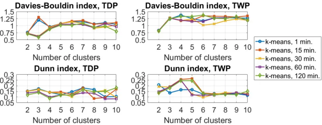
The DB and the DI for the different temporal resolutions and number of clusters k can be seen in figure 1. For most resolutions, two clusters are optimal for the TWPs while three clusters are optimal for TDPs. Clustering TWPs is more robust for different temporal resolutions according to DB, while clustering TDPs is more robust according to DI. No temporal resolution outperforms any other, but DB shows slightly better values for lower temporal resolution. DI has a better value in most cases for TWP rather than TDP, which stands in contrast to DB.
The average TDP and TWP for the clusters when k=2 can be seen in figure 2. Cluster 1 is always the largest cluster and cluster 2 is always the second largest cluster. However, when clustering TWPs the number of customers in each cluster is very even. Compared to several other studies on clustering load data [3-9,11,16], the optimal number of clusters is relatively low, suggesting fairly homogeneous customers. However, it is not the only study where two or three is the optimal number of clusters [14,15].
The different average load profiles will be denoted flat and curvy clusters, respectively, derived from the appearance of each average profile. Most customers end up in the flat TDP cluster both when k=2. For the TWPs when k=2 most customers end up in the curvy cluster, with exception for the temporal resolution 60 minutes.
When k=3 the flat clusters always has the most customers, followed by the curvy cluster. The third new cluster contains the customers which are on the limit on either being in the flat or curvy cluster. For TWPs, the curvy cluster has an even more clear reduction during the weekends, while the third new cluster has a higher average use on Saturdays than Sundays, but significantly lower than the weekdays.
The curvy clusters show a clear reduction in use during nights and weekends. The flat clusters show no daily or weekly patterns, but has an average profile which fluctuates slightly around a relatively high and stable use. The curvy TWP clusters shows a tendency of lower electricity use on Fridays than the other weekdays. For the curvy TDP clusters, a small reduction in electricity use around 8:00am is visible for temporal resolution from 1 to 30 minutes.
The number of customers who change between the flat and the curvy depending on whether they are clustered with TDP or TWP can be seen in table 1. This corresponds to 11-14 % of the customers when
k=2 and 25-28 % when k=3. When k=2, most customers who change cluster are in the flat cluster when
clustering after their TDP and in the curvy when clustering after their TWP. When k=3, most customers who change cluster are in the flat or curvy cluster when clustering after their TDP and in the third new cluster when clustering after their TWP. Saturdays' electrical use is on average higher than Sundays' for the customers who change cluster but lower than the weekdays.
Figure 2: The average TDP and TWP for cluster 1 and 2, respectively, when k=2. The TWPs start at Thursdays 00:01am. Cluster 1 is always the largest cluster and cluster 2 is always the second largest cluster.
Table 1: Number of customers who change cluster depending on if clustering is done for their TDP or TWP.
Temporal resolution (minutes)
1 15 30 60 120
Number of customers who
change cluster when k=2 14 15 13 12 14 Number of customers who
change cluster when k=3 31 26 26 26 26
4. Conclusions
When clustering after the typical daily profiles (TDPs) some customers with a clearly weekly pattern, are clustered together with customers who have an even load. Especially when divided into three clusters, numerous customers change cluster depending on if they are clustered after their TDP or typical weekly profile (TWP). Those customers seem to have electrical equipment turned on during Saturdays.
Depending on the application, using a TWP could be more suitable than using a TDP. If this causes problems due to large data sets, it can be fitting to aggregate the data to lower temporal resolutions. In this study, no signs of improved results for higher temporal resolutions when clustering load profiles were found. Number of clusters effected the performance evaluators more.
Clustering could be used for improved forecasting, distribution planning or tariff design. Knowing if a customer uses electrical equipment on all days or only some days during the weeks can be relevant for all of these applications. When forecasting, it could be advantageous to have customers with different electricity use on Saturdays in different cluster to forecast the weekends and especially Saturdays correctly. If implementing Time-of-Use tariffs, which is a pricing scheme used to increase demand side management, clustering customers after their TWP could reveal if it is advantageous with different tariffs during the weekends.
Acknowledgements
The authors would like to thank Svenska Energigruppen and eSmart Scandinavia for contributing with data. The work has been carried out under the auspices of the industrial post-graduate school Reesbe, which is financed by the Knowledge Foundation (KK-stiftelsen).
References
[1] K. Zhou, C. Fu, S. Yang, Big data driven smart energy management: From big data to big insights, Renewable and Sustainable Energy Reviews 56 (2016) 215-225.
[2] I. Panapakidis, M. Alexiadis, G. Papagiannis, Load profiling in the deregulated electricity markets: A review of the applications, in: 2012 9th International Conference on the European Energy Market, IEEE, 2012, pp. 1-8.
[3] M. Espinoza, C. Joye, R. Belmans, B. De Moor, Short-term load forecasting, profile identification, and customer segmentation: a methodology based on periodic time series, IEEE Transactions on Power Systems 20 (3) (2005) 1622-1630.
[4] S. Ramos, J. Duarte, J. Soares, Z. Vale, F. J. Duarte, Typical load profiles in the smart grid context – a clustering methods comparison, in: Power and Energy Society General Meeting, 2012 IEEE, IEEE, 2012, pp. 1-8.
[5] D.-W.-I. C. Flath, D.-W.-I. D. Nicolay, T. Conte, P. D. C. van Dinther, L. Filipova-Neumann, Clusteranalyse von Smart-Meter-Daten, Wirtschaftsinformatik 54 (1) (2012) 33-42.
[6] Y.-I. Kim, J.-M. Ko, S.-H. Choi, Methods for generating TLPs (typical load profiles) for smart grid-based energy programs, in: 2011 IEEE Symposium on Computational Intelligence Applications In Smart Grid (CIASG), IEEE, 2011, pp. 1-6.
[7] G. Chicco, Overview and performance assessment of the clustering methods for electrical load pattern grouping, Energy 42 (1) (2012) 68-80.
[8] A. Lavin, D. Klabjan, Clustering time-series energy data from smart meters, Energy E-ciency 8 (4) (2015) 681-689. [9] R. Granell, C. J. Axon, D. C.Wallom, Impacts of raw data temporal resolution using selected clustering methods on residential electricity load profiles, Power Systems, IEEE Transactions on 30 (6) (2015) 3217-3224.
[10] A. Shahzadeh, A. Khosravi, S. Nahavandi, Improving load forecast accuracy by clustering consumers using smart meter data, in: Neural Networks (IJCNN), 2015 International Joint Conference on, IEEE, 2015, pp. 1-7.
[11] T. Räsänen, D. Voukantsis, H. Niska, K. Karatzas, M. Kolehmainen, Data based method for creating electricity use load profiles using large amount of customer-specific hourly measured electricity use data, Applied Energy 87 (11) (2010) 3538-3545.
[12] F. McLoughlin, A. Duffy, M. Conlon, A clustering approach to domestic electricity load profile characterisation using smart metering data, Applied energy 141 (2015) 190-199.
[13] A. Al-Wakeel, J. Wu, K-means based cluster analysis of residential smart meter measurements, Energy Procedia 88 (2016) 754-760.
[14] E. Pan, H. Li, L. Song, Z. Han, Kernel-based non-parametric clustering for load profiling of big smart meter data, in: Wireless Communications and Networking Conference (WCNC), 2015 IEEE, IEEE, 2015, pp. 2251-2255.
[15] R. Al-Otaibi, N. Jin, T. Wilcox, P. Flach, Feature construction and calibration for clustering daily load curves from smart meter data.
[16] T. Räsänen, M. Kolehmainen, Feature-based clustering for electricity use time series data, in: International Conference on Adaptive and Natural Computing Algorithms, Springer, 2009, pp. 401-412.
[17] J. MacQueen, et al., Some methods for classification and analysis of multivariate observations, in: Proceedings of the fifth Berkeley symposium on mathematical statistics and probability, Vol. 1, Oakland, CA, USA., 1967, pp. 281-297.
[18] D. L. Davies, D. W. Bouldin, A cluster separation measure, Pattern Analysis and Machine Intelligence, IEEE Transactions on (2) (1979) 224-227.
[19] J. C. Dunn, Well-separated clusters and optimal fuzzy partitions, Journal of cybernetics 4 (1) (1974) 95-104. [20] Mathworks, k-means clustering - MATLAB kmeans, http://se.mathworks.com/help/stats/kmeans.html, 2016-05-20. [21] Mathworks, Evaluate clustering solutions - MATLAB evalclusters, http://se.mathworks.com/help/stats/evalclusters.html, 2016-05-20.
[22] Ilc, N., Modified & Generalized Dunn's index, https://www.mathworks.com/matlabcentral/fileexchange/42199-modified---generalized-dunn-s-index, 2016-06-22.
Biography
Anna has a B.Sc. in Engineering Mathematics and a M.Sc. in Sustainable Energy Systems from Chalmers University of Technology in Sweden. Currently she is an industrial PhD student in the graduate school Reesbe and employed by Svenska Energigruppen AB in cooperation with Mälardalen University. Her research interests include Smart Grids and Data mining in energy systems.