School of Innovation Design and Engineering
V¨
aster˚
as, Sweden
Thesis for the Degree of Master of Science in Engineering - Software
Engineering 15.0 credits
AUTOMATION AND EVALUATION
OF SOFTWARE FAULT PREDICTION
Bora Lam¸ce
ble17001@student.mdh.se
Examiner: Federico Ciccozzi
M¨
alardalen University, V¨
aster˚
as, Sweden
Supervisor: Wasif Afzal
M¨
alardalen University, V¨
aster˚
as, Sweden
Acknowledgments
First and foremost, I would like to express my deep and sincere gratitude to my supervisor, Wasif Afzal, who has provided me with unlimited guidance, recommendations and advice during this thesis work. It was through his dedication and supervision that this thesis came to life. I am thankful to his support during our meetings.
Besides, I would like to thank the EUROWEB+ Scholarship Programme for giving me the possibility to further my studies at M¨alardalen University. I am grateful to M¨alardalen University for making it easier for me to restart the academical path. The excellent educational system and infrastructure they provide motivated me to further proceed with this thesis work.
Last but not least, I am extremely grateful to my dearest ones for always encouraging and supporting me in my work. Most of all, I am grateful to my brother, who brightens up my everyday making it easier to work on this thesis.
Abstract
Delivering a fault-free software to the client requires exhaustive testing, which in today’s ever-growing software systems, can be expensive and often impossible. Software fault prediction aims to improve software quality while reducing the testing effort by identifying fault-prone modules in the early stages of development process. However, software fault prediction activities are yet to be implemented in the daily work routine of practitioners as a result of a lack of automation of this process. This thesis presents an Eclipse plug-in as a fault prediction automation tool that can predict fault-prone modules using two prediction methods, Naive Bayes and Logistic Regression, while also reflecting on the performance of these prediction methods compared to each other. Evaluating the prediction methods on open source projects concluded that Logistic Regression performed better than Naive Bayes. As part of the prediction process, this thesis also reflects on the easiest metrics to automatically gather for fault prediction concluding that LOC, McCabe Complexity and CK suite metrics are the easiest to automatically gather.
Table of Contents
1 Introduction 7
1.1 Motivation & Problem Formulation . . . 7
2 Background 9 2.1 Software Fault Prediction . . . 9
2.2 Software fault information . . . 10
2.3 Software metrics . . . 10
2.4 Fault prediction techniques . . . 11
2.4.1 Statistical Methods . . . 11
2.4.2 Machine Learning Methods . . . 12
2.5 Prediction Method evaluation . . . 13
2.5.1 WEKA 10-folds cross-validation . . . 13
2.5.2 Confusion Matrix . . . 13 2.5.3 Precision . . . 13 2.5.4 Recall . . . 14 2.5.5 F-measure . . . 14 2.5.6 ROC Curve . . . 14 2.5.7 Precision-Recall Curve . . . 15 3 Related Work 16 4 Method 17 4.1 Construct a Conceptual Framework . . . 17
4.2 Develop a Plug-in Architecture . . . 17
4.3 Analyze and design the Plug-in . . . 17
4.3.1 Software Metrics Identification . . . 17
4.3.2 Project Identification . . . 18
4.3.3 Prediction Methods Identification . . . 18
4.4 Build the plug-in . . . 19
4.5 Experimentation, Evaluation and Observation . . . 19
4.5.1 Experimentation . . . 19
4.5.2 Evaluation . . . 19
4.5.3 Observation . . . 19
5 A Reflection on Metrics Gathering 20 6 A Software Fault Prediction Tool 22 6.1 SFPPlugin Components . . . 22
6.2 SFPPlugin Users Perspective . . . 23
6.3 SFPPlugin Advantages . . . 27
7 Prediction Method Evaluation Results 28 7.1 Incorrectly classified instances . . . 28
7.2 Confusion Matrix Rates . . . 29
7.3 Precision Rates . . . 30
7.4 Recall Rates . . . 32
7.5 F-measure Rates . . . 33
7.6 Area under ROC curve . . . 33
7.7 Area under PR curve . . . 34
7.8 Result Summary . . . 34
9 Limitations 38 9.1 Study design limitations . . . 38 9.2 Data limitations . . . 38 9.3 Impact limitations . . . 38
10 Conclusions and Future Work 39
List of Figures
1 Research question work flow . . . 8
2 Software fault prediction process . . . 9
3 ROC curve illustrations . . . 14
4 SFPPlugin flow graph . . . 23
5 Enable Fault Prediction . . . 23
6 Training data . . . 24
7 Show Fault Prediction View . . . 25
8 Fault Prediction View . . . 25
9 Fault Prediction Results View . . . 26
List of Tables
1 Confusion Matrix example . . . 13
2 List of tools for metric gathering . . . 20
3 Arff attribute description . . . 22
4 Data distribution . . . 28
5 Incorrectly classified instances . . . 29
6 Classification result table . . . 30
7 Precision result table . . . 31
8 Recall result table . . . 32
9 F-Measure result table . . . 33
10 Area under ROC result table . . . 34
11 Area under PR Result Table . . . 35
12 Result summary according to datasets . . . 35
13 Result summary according to performance measures . . . 36
14 All versions composed datasets performance compared to single versions datasets performance . . . 36
1
Introduction
A great amount of the software development budget is dedicated to software testing and to quality assurance activities [1]. Consequently, this indicates the importance of testing during the software development lifecycle. Through the years, software systems have grown to be larger and more complex, thus making the task of providing high-quality software more difficult. Software engineers’ aim is to deliver a bug-free software to the end user. To acquire such confidence, the software needs to be exhaustively tested, resulting in an expensive, tedious and, sometimes, an impossible task. Testing is often limited due to resources and time restrictions. Predicting fault-prone code helps practitioners focus their resources and effort on the fault-prone modules, thereby improving the software quality and reducing the maintenance cost and effort [2]. Software fault prediction makes it possible to detect faulty code during software development and prevents faults from propagating in other parts of the software. Moreover, it is a process that helps optimize testing by focusing on fault-prone modules, identifying the refactoring candidates and improving the overall quality of the software [3].
Project managers can greatly benefit from software fault prediction. They can measure the quality of the work during the development phases by continuously measuring the fault-proneness of a module. Through fault prediction, the project manager can detect the needs for refactoring and assign tasks based on that information and therefore improving the efficiency of the process. Fault prediction related issues are classified by Song at al. [4] in three main categories:
1. Evaluating the number of faults still present in the system; 2. Investigating the correlation between different faults;
3. Classifying system modules as fault-prone or non-fault-prone.
This thesis focuses its work on the third issue presented above. This issue presents the ability to mark a module as fault-prone or non-fault-prone and thus providing the developers with an insight of how the quality assurance activities should be oriented. To enable this classification, researchers, through the years, have used statistical and machine learning methods.
The process of prediction is intuitive and easy to understand. A prediction method learns how the system behaved previously through historical attributes of the system (metrics) and historical bug reports. At this point, the model knows that faulty modules will manifest certain attribute values. Baring this information, the model can classify the modules of the current version of the system as fault-prone or non-fault-prone
However, this process is far from perfect and reliable. There are still many issues for which we can not find a definitive answer i.e What are the attributes that guarantee the best predictions and how to collect them? What is the best way to collect bug reports and, most importantly, what are the best methods for fault prediction? These questions include an extensive area of study that is well beyond the scope of this thesis. The focus of this thesis is the study of automated metrics collection process, the evaluation of fault prediction models and the development of a usable fault prediction tool.
1.1
Motivation & Problem Formulation
Files and classes containing faulty code can be detected by analyzing data collected from previous releases of a project, or if no previous releases exist, data collected from similar projects. An important part of achieving successful fault prediction in a project is the selection of the metrics and techniques used to predict the faults. Fault prediction metrics, techniques, and methods have been widely studied during past years [5] [6] [7]. This study aims to develop a software fault prediction tool, evaluate two prediction methods with respect to prediction performance and to reflect on the ease of gathering software metrics. Guo et al. [8] suggested the need for a similar tool in 2004 where software development organizations are encouraged to analyze their own data repositories for better fault detection.
Building this tool provides a perspective on all the stages of the software fault prediction process. From the selection of the open source projects, the selection and evaluation of the easiest metrics to use, the collection of these metrics, the selection and evaluation of the prediction methods, and
the implementation of these methods. This all will result in a software prediction tool that can be later incorporated in the practitioners’ daily routine.
The aim of this thesis is to automate the process of fault prediction, to evaluate the performance of two fault prediction methods using the automated solution and reflect on the ease of gathering software metrics. The prediction methods will be evaluated based on prediction performance [9] on open source projects using measures such as Precision, Recall, F-measure, Area Under Curve (AUC) and Area Under Precision-Recall Curve. These measures will be described in Section2.5.
In order to reflect on automating the prediction process, the thesis will investigate which metrics are easy candidates for collection to make predictions.
This thesis evaluates two of the most known software fault prediction methods (Naive Bayes and Logistic Regression) in an environment that can potentially be used on an everyday workspace for software developers such as Eclipse. Eclipse IDE is an open source and widely used development environment [10] and thus can be a useful solution for many developers. This is the main motivation behind the decision to develop the Eclipse plug-in during this thesis and to evaluate the prediction methods facilitated by the plug-in implementation.
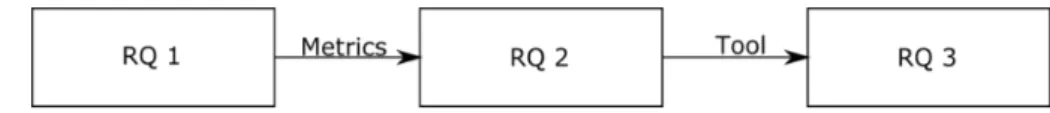
The problem formulated in this section is summarized by the following research questions. • RQ 1: Which metrics are easy candidates for automatic collection for software faults
pre-diction?
• RQ 2: How can we implement an open source available tool for software fault prediction that integrates with developers’ integrated development environment (IDE)?
• RQ 3: Which of the implemented fault prediction methods perform the best when using the implemented tool?
In RQ1, we will reflect on our experience during the process of gathering metrics. In RQ2, we will demonstrate the implementation of an open source prediction tool that can be available and integrated into the developers’ environment. In RQ3, we will evaluate the performance of the prediction methods using the implemented tool on open source data. All three RQs are strongly related to each other as the output for the previous is used as the input for the next. The work flow of this thesis in terms of these RQs is presented in Figure1.
2
Background
This section presents a background to the software fault prediction problem, software metrics, fault prediction techniques and prediction model evaluation.
2.1
Software Fault Prediction
Software fault prediction is the process of improving the software quality and testing efficiency by early detection of fault-prone modules. This process reduces testing effort while still ensuring software quality. Based on the predictions gathered from the fault prediction process, project managers can organize their resources in a way that focuses the majority of the testing effort in the modules marked as fault-prone [11].
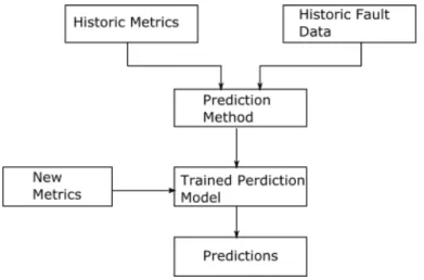
As a result of the software fault prediction process, the software modules are classified as fault-prone or non-fault-prone. The modules are classified by classification methods based on the software metrics and fault information gathered from previous releases of the software [2]. In other words, software attributes, and previously reported fault information collected in the software’s previous releases are used to train prediction methods that can later classify a module in the new version as fault-prone or not fault-prone. Thus, whenever an error is reported in a module in the old versions of the software, that module is marked as faulty and its metrics are measured. This information is then provided as training data to the prediction model that uses it to forecast the fault-proneness of that module in the new releases [12].
Figure 2: Software fault prediction process
Fault prediction is key in elevating the quality of a software while still optimizing the costs of the resources. By using fault prediction tools, the project manager can allocate the most resources to the modules that are classified as fault-prone. Early detection of the faults is thereby, cost-effective and minimizes the maintenance effort for the system [11].
The task of predicting fault-prone modules can be complex. The process of gathering data from previous versions of the software can be time-consuming, tedious and error-prone. With the intention of simplifying this process, several automation gathering tools have been proposed through the years. However, the challenges are not done yet, the data gathered is often imbalanced where most of the modules are marked as not faulty and what about the projects that do not have any previous metrics or fault data, the projects that just have started their development. Gathering good training data is crucial to the quality of the predictions.
The most important components in a software fault prediction process are software fault data, software metrics, and fault prediction techniques. To gather a better understanding of the process the next section will provide a brief description of each one these components [13].
2.2
Software fault information
Software fault information contains all the information about the faults reported during the soft-ware life-cycle. Version control systems are used to store source code and change management systems are used to store the fault data reported [12]. The datasets containing source code infor-mation are listed according to their availability [5].
• Private: The datasets are not publicly available. Neither the source code or the fault in-formation can be accessed. The studies concluded that these types of data sets are not repeatable.
• Partially public: Only the source code and the fault information are available, but the code metrics are not available. In this case, the author has to extract the metrics from the code and match them to the fault information. This is the case in our study since the tool is to be used in the organization’s repositories where they have access to their source code and fault information but the metrics have to be calculated for the sake of the fault prediction. • Public: The source code, fault information, and metrics are available to be used publicly [5]. One of the major issues regarding fault data in the source dataset is imbalanced data. The majority of the modules are labeled as non-fault-prone whereas the remaining part is labeled as fault-prone. Thus, data distributed this way can affect the fault prediction methods performance. Nevertheless, to deal with this issue, it is often recommended to oversample the minority in order to balance the data [14]. Regardless of this, in this thesis, we did not use any techniques to improve imbalanced data. The reason for this is that our tool is meant to be used in the real world where we do not have an insight into the balance of the data. Implementing techniques of data balancing may affect datasets that are not imbalanced.
2.3
Software metrics
Software metrics represent the values of measurements on software attributes. Metrics are used for quality assurance, performance measurements, debugging, cost estimation. Most importantly, they are vital to the process of fault prediction [15]. Different metrics can be used in software fault prediction and they are categorized as follows [5]:
• Traditional Metrics: This category includes metrics mostly based on the size and complexity of the program:
– LOC (Line of codes) - Is the most basic metric and calculates the number of executable instructions in the source code. Many studies have shown a moderate correlation be-tween the lines of code in a module and the faults present in that module [5].
– McCabe Cyclomatic Complexity (MCC) [16] metric - Cyclomatic complexity is a source code complexity measurement that is calculated by measuring the number of linearly-independent paths through a program module. The average value of the Cyclomatic Complexity can help identify whether or not a class is more prone to faulty behav-ior [11]. Cyclomatic complexity was fairly effective in large post-release environments using Object-Oriented languages but not in small pre-release environments with proce-dural languages [5].
– Halstead [17] - Halstead measures the program vocabulary, length, effort, difficulty through the number of operands and operators present. Halstead’s metrics reported poor results and were estimated inappropriate for fault prediction [5].
• Object-Oriented Metrics: Object-Oriented metrics are the most used metrics in the studies of fault prediction. They are designed to measure attributes of source code developed in Object-Oriented languages. One of the most used is the Chidamber and Kemerer suite [18]. The CK suite includes these metrics:
– Coupling between objects CBO - Measures the degree to which methods declared in one class use the instance variables or methods defined in another class.
– Depth of an inheritance tree DIT - The distance of this object from the base class (Object) in the inheritance tree.
– Response for a class RFC - It is defined as the sum of the number of methods in one class and the number of remote methods called by this class.
– Weighted methods per class WMC- Is an object-oriented metrics that measures the complexity of a class. It is often calculated as the sum of the complexity of all the methods included in the class.
– Number of children - Is calculated as the number of immediate subclasses in the class hierarchy.
– Leak of cohesion of methods - Measures the dissimilarities between the methods in one class.
Object-oriented metrics are considered as good fault predictors [5].
• Process Metrics: Are metrics like process, code delta, code churn, history and developer metrics. These metrics are usually extracted from the combination of source code and repos-itory [5] [19].
2.4
Fault prediction techniques
Fault prediction techniques are classifiers that use inputs such as previous fault information and software metrics to classify the current modules of the system as fault-prone or non-fault-prone. In the literature, there are two well-known categories of prediction methods: Statistical Methods and Machine Learning Methods. We will now describe one representative method for each of these categories.
2.4.1 Statistical Methods Logistic Regression
Logistic regression [20] is the most commonly used statistical method [21]. This method can predict the dependent variable from a set of independent variables. We are interested in using binary logistic regression. In binary logistic regression, the dependent variables tend to be binary, just as in our case where we are trying to define if one module is faulty or not. The independent variables that can be used to predict the faulty modules are the metrics described above. There are two types of logistic regression, univariate logistic regression and multivariate logistic regression.
• Univariate logistic regression formulates a mathematical model that represents the relation-ship between the dependent variable and each of the independent variables.
• Multivariate logistic regression is what is used to construct a fault prediction model. In this method, the metrics are used in a combination. Multivariate logistic regression is calculated in the Equation1
prob(X1, X2, ..., X3) =
e(A0+A1X0+...+AnXn)
1 + e(A0+A1X0+...+AnXn) (1)
Where prob is the probability of a module being classified as faulty and Xi are the
indepen-dent variables. Univariate logistic regression is just a special case an in the Equation2 prob(X1, X2, ..., X3) =
e(A0+A1X0)
1 + e(A0+A1X0) (2)
There are two methods that can be used for the selection of the independent variables. The Forward selection which examines the variables one by one at the time of entry. Backward elimi-nation, on the other hand, includes all the variables to the model from the start. It then deletes the variables one by one until a stop criterion is fulfilled. The backward elimination is reported to perform slightly better than the forward selection in the fault prediction problem [21].
This thesis is using the Logistic Regression implementation provided by WEKA 1 API in the
classifier SimpleLogistic [22] [23]. In this classifier builds a multivariate, forward selection linear logistic regression model.
2.4.2 Machine Learning Methods
Machine learning methods make use of example data or past algorithms to solve a given prob-lem [24]. In our study, we want to use machine learning to predict whether a specific module will be faulty or not based on the previous fault data collected and the metrics collected from the project.
Naive Bayes Classifier
Naive Bayes is a classifying machine learning technique that is not only easy to implement but also very efficient in the fault prediction problem [3]. Grounded on the Bayesian Theorem, this method will rule if an object is part of a specific category based on the features of that object. Similarly, for the software fault prediction model, the method classifies the modules as fault-prone or non-fault-prone based on the metrics measured in the modules [25]. Moreover, the Naive Bayesian Theorem states as follows in Equation3
P (C|F1, F2, ..., Fn) =
P (C)P (F1, F2, ..., Fn|C)
P (F1, F2, ..., Fn)
(3) Where:
• P (C|F1, F2, ..., Fn) is the probability of observing a certain category, faulty or non-faulty,
given certain values of metrics.
• P (C) is the probability of observing a certain category, faulty or non-faulty.
• P (F1, F2, ..., Fn|C) is the probability of encountering these metric values in this specific
cat-egory.
• P (F1, F2, ..., Fn) is the probability of observing these metric values alone.
Assuming independence so that the metrics are independent from each other, equation 4 can be written:
P (C|F1, F2, ..., Fn) ∼ P (C)prodni=1P (Fi|C) (4)
The probability of observing the category of faulty or non-faulty given the metric values is proportional to the probability of observing this category multiplied by the probability of observing metric 1 (F1) in the category C multiplied by the probability of observing the metric 2 (F2) in the category C and so on for each feature F.
What the Naive Bayes classifier does is that whenever a new module is introduced to the new releases, it can calculate based on its metrics, the likelihood that this module is faulty or not. It will then compare the probabilities of the two classes and the one with the largest value is the category that is predicted.
cassif y(f1, f2, ..., fn) = maxargP (C = c)prodni=1P (Fi= fi|C = c) (5)
The model is first fed with training data which include the calculations of the metrics for the modules in the project and the information whether or not these modules resulted faulty in previous releases. Later in the process, this data is used to predict whether in the new release the modules will be faulty or not.
This thesis is using WEKA’s API implementation for Naive Bayes in the class appropriately named NaiveBayes [26].
2.5
Prediction Method evaluation
This section is dedicated to the description of the methods and measures used to evaluate the performance of the prediction methods. The prediction methods are evaluated using an implemen-tation of WEKA API 10-fold cross-validation into the proposed fault prediction tool. From the cross-validation results, we have extracted the following measurements to use in the evaluation of the prediction methods. Selection of these evaluation measurements is based on previous studies on that rank the best measures to use in the context of fault prediction models evaluation [9]. 2.5.1 WEKA 10-folds cross-validation
Cross-validation is a statistical method used to evaluate machine learning algorithms. During the evaluation, the dataset is divided into two main segments: one segment used for training the model and the other segment used for testing classification of the model. The most common form of cross-validation is the k-fold cross-validation. This kind of validation divides the dataset into k equal folds. The first k-1 folds are used to train the model while the last fold is used to test the prediction computed by the prediction method. This process is repeated k times to ensure that the training and testing sets are crossed over and the data points are validated [27].
In the software fault prediction tool, we used WEKA’s 10-fold cross-validation. The dataset provided is segmented into ten equal folds. Additionally, WEKA stratifies the data. This means that the data is rearranged to ensure a uniform distribution of each class. Nine out of the ten folds train the prediction model. Later, the trained model is used to predict fault-proneness in the last fold. The results gathered from the prediction of the last fold are compared with the real classes of the fold and the evaluation metrics are computed. These steps are repeated ten times.
2.5.2 Confusion Matrix
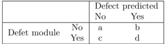
All the necessary information for the prediction models evaluation is found in a confusion ma-trix [28]. This matrix contains information about the instances classified by the predictor and how they relate to the real class of the instances. The data gathered by this matrix is later used to calculate numerical or graphical evaluations. The data gathered in such matrix [29] are presented in Table1.
• a - The number of non-faulty modules predicted correctly (true negative). • b - The number of non-faulty modules predicted incorrectly (false positive). • c - The number of faulty modules predicted incorrectly (false negative). • d - The number of faulty modules predicted correctly (true positive).
Defect predicted
No Yes
Defet module No a b
Yes c d
Table 1: Confusion Matrix example
2.5.3 Precision
Precision is the rate of correctly classified instances from all the instances classified in that class [9]. In the fault prediction problem, precision is the rate of correctly identified faulty modules from all the instances classified as faulty as in Equation6. The same logic is valid for non-faulty predictions in Equation7.
P recisionF aulty=
Correctly F aulty Classif ied Instances
P recisionN on−F aulty =
Correctly N on − F aulty Classif ied Instances
Overall N on − F aulty Classif ied Instances (7) 2.5.4 Recall
Recall or Probability of Detection (PD) is the rate of correctly classified instances from all the instances of that class [9]. In the fault prediction problem, Recall is the rate of correctly identified faulty modules from all the real faulty modules as in Equation 8. The same logic is valid for non-faulty predictions in Equation9.
RecallF aulty=
Correctly F aulty Classif ied Instances
Overall F aulty Instances (8)
RecallN on−F aulty =
Correctly N on − F aulty Classif ied Instances
Overall N on − F aulty Instances (9)
2.5.5 F-measure
F-measure [30] integrates Recall and Precision. In addition, it also includes a weight factor β which is used to regulate the weight given to Recall.
F − measure = (β
2+ 1) × P recision × Recall
β2× P recision + Recall (10)
β is set to 1 when the weight of Precision and Recall is the same. In the other cases, a bigger β indicates a bigger Recall weight. β provides this measure with a better flexibility than the ones mentioned previously by manipulating the cost assigned to Recall and Precision [29].
2.5.6 ROC Curve
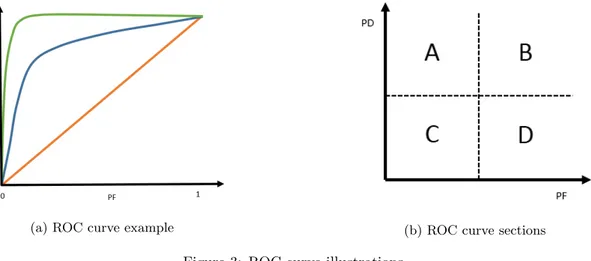
In general, in module classification, a higher True Positive Rate (TP) will always be at the expenses of a higher False Positive Rate (FP) and the other way around. The true positive rate represents the probability of detection of a faulty module and the false positive rate is the portion of non-faulty-modules that are classified as fault-prone. Receiver Operating Characteristic (ROC) Curve depicts the relationship between the TP and FP and is a graphical generalization of the more numerical measurements discussed above [31]. It offers a visual representation of the probability that a classifier will correctly classify a module as faulty and the probability that this classification is a false alarm.
(a) ROC curve example (b) ROC curve sections
Figure 3: ROC curve illustrations
Figure3ais a graphical example of how the ROC Curve may look. The orange line represents a random classification. A classifier who labels the modules as fault-prone or non-fault-prone purely
based on randomness will provide us with a similar looking ROC graph. The green line is an ideal classification where all the modules are correctly classified. This represents the best classifier that we can use. Whereas the blue line represents a more realistic view of the ROC curve. This is the kind of curve that we are hoping to see during the evaluation of the fault prediction methods used in this study.
A numeric representation of the ROC curve is AUC (Area Under a Curve) which is often written as the area under the ROC curve. Therefore, this evaluation method is directly connected to the ROC method. Additionally, not all regions under a curve are interesting for the software prediction problems. The figure3brepresents the four main regions in a ROC graph. The region with low rates of True Positives (Region C), the region with high rates of False Positives (Region B), or both indicates poor performance for the classification models. Thus, it is desirable that a classification method indicates the highest value under the area A. Studies [9] have shown that the area under region A is a more reliable measurement of the performance of the method than the area under the entire curve of ROC.
2.5.7 Precision-Recall Curve
Another way to graphically assess the quality of the classifiers is by using a Precision-Recall Curve. This curve depicts the relationship between the Precision in the y-axis and the Recall, also known as the True Positive rate, in the x-axis. The area of most interest in this curve is the one where there are a high recall and a high precision rate. According to studies [9], this curve may reveal deeper performance differences between the classifiers. In spite of that, this is not a better evaluator than ROC curve but it comes in handy when the results form the ROC curve are not conclusive enough.
3
Related Work
A wide range of studies provides evidence about the most successful methods, metrics, and tech-niques used to achieve good software fault prediction. All these studies provide a good body of knowledge and share lessons learned for those who want to adopt fault prediction in practice [15]. In this section, we decided to review mostly literature review studies since we feel that they include all the necessary progress made in this area. All literature review papers below are presented in a chronological order according to the publishing date.
The main purpose of Wahyudin et al. [15] study was to provide a review for existing studies in the software fault prediction area in order to facilitate the use of software fault prediction in a particular organization or project. They proposed a framework that takes care of this problem. They concluded that many of the reviewed studies did not take into account the problem of missing fault information that many practitioners face in their projects and thus, they provide incomplete results. An important issue raised in this paper is that, apart from the results provided to the practitioners by the prediction models, they also need an additional measure to indicate the reliability of these results. They need to be sure that they are not endangering product quality by missing critical defects because the prediction falsely labeled a module as non-fault-prone.
Catal [3] reviewed the most relevant studies from 1990 up to 2009 in terms of the fault prediction method they used, metrics they selected and the source code they used. This literature review concluded that in most of the studies, the most popular metrics were method level metrics and the most popular prediction models where the machine learning models. They also identified Naive Bayes as a robust machine learning mechanism for software fault prediction.
Hall et al. [32] reviewed 36 studies with the main intention of discovering what impacts the prediction model performance. This study found evidence that the models performed better in larger contexts and that the maturity level does not have any effect on the performance of the model. A combination of static, process and Object-Oriented metrics helped the prediction models perform better. Process metrics alone did not perform as well as expected and the Object-Oriented metrics performed best. Naive Bayes and Logistic Regression are the modeling techniques that gave the best results.
According to Radjenovi´c et al. [5], the performance of a software prediction model is influenced mostly by the choice of the metrics. The difference in performance between different techniques is not relevant but the difference of performance for different metrics is considerable. This study aimed to depict the state-of-art available on the metrics in software failure prediction. They studied 206 studies. The overall effectiveness of size metrics was estimated as moderate with a stronger correlation with pre-release studies and small projects. The complex metrics were not considered bad fault predictors with the McCabe metric leading the category. Moreover, the Halstead metrics did not provide effective results. Finally, the object-oriented metrics are the most used and the most effective. More specifically, the CK metric suite provided the highest performance among Object-Oriented metrics. Some of the CK metric suite where classified as not reliable. The MOOD and QMOOD metrics provided poorer performance. Process metrics resulted more likely to predict post-release faults.
Malhotra [6] on the other hand studied the machine learning techniques used for fault prediction. In this study, it was clear that Machine Learning techniques outperform the other statistical techniques. The best performance metrics were the Object-Oriented metrics in compliance with the other studies in this area. Malhotra also stated that the application of the machine learning techniques in software fault prediction is still limited and they encouraged new studies to be carried out in order for the results to be easily generalized.
Based on the findings of the different literature reviews for the fault prediction problem our study aims to introduce a software fault prediction tool built on the prediction methods known to literature to perform the best. Furthermore, this study will contribute to the body of knowledge of the prediction methods performance by evaluating the Naive Bayes and Logistic Regression predictors when used in our tool. Through this process, we will also pay close attention to the metrics that are the easiest to be collected.
4
Method
In order to address the problem in Section 1.1, the thesis is conducted according to the system development methodology presented in [33]. It should be noted that although it is a development methodology, there is an evaluation component of the methodology (step 5), covering the evaluation of prediction performance. Moreover, in the analysis and design of the system (step 3 below), the thesis reflects on the ease of capturing the metrics used for making predictions. The system developed is an Eclipse Plug-in thus from now one we will refer to the system as the plug-in.
The following steps in the plug-in development methodology are carried out:
4.1
Construct a Conceptual Framework
The construction of a conceptual framework in this thesis work is concerned in building a solid knowledge of the problem’s domain and creating and stating meaningful research questions that help shape the rest of the work. To present a solid state-of-art knowledge, we aimed at reviewing the most important studies in software fault prediction, metrics used for software fault prediction and prediction methods. For the purpose of this thesis, we decided to focus our main attention to the literature review studies on software fault prediction. We argue that the literature review studies depict a clear picture of the studies conducted through the years in the software fault prediction area. Furthermore, through these studies, we identified the most relevant papers to our thesis and discarded the most non-relevant ones.
The collection of the software fault prediction literature studies was conducted through the databases “Scopus” and “IEEExplore”. In both databases, the query used to find the papers was: “software fault prediction” OR “software defect prediction” OR “bug prediction” AND “liter-ature review”
Each collected paper is considered relevant if it concerns one of our main topics i.e: software fault prediction, software metrics or prediction methods. Moreover, we only considered papers written in English and that presented final results for each study reviewed. All the relevant papers collected through this process are reviewed thoroughly and the findings are presented in the Section3.
Lastly, in light of the knowledge gathered, this thesis is focusing on responding to the three research questions presented in Section 1.1
4.2
Develop a Plug-in Architecture
This phase is dedicated to designing a solution for the problem stated in the previous phase. The aim of this thesis is to answer all three research questions presented in Section 1.1through the development of a software fault prediction tool.
The proposed tool is an Eclipse plug-in that can predict faulty modules in Java developed projects. The environment and the language chosen are both very commonly used, thus providing a solution for many developers. Furthermore, this combination is also very comfortable given the author’s knowledge and experience, thus increasing the chances of achieving quality results.
4.3
Analyze and design the Plug-in
In this phase, we analyze the requirements and the design of the tool.
Now it is important to define what will the tool measure and how will the results be produced and measured. As discussed in the Section2.1, there are three major components in the software fault prediction process: software metrics, fault data, and prediction methods. During the design process, we carefully weighed the options for each component.
4.3.1 Software Metrics Identification
For the identification of the metrics to be used by the prediction tool, we first identified all the software metrics used for software fault prediction throughout the literature. All the metrics were then categorized according to the type of measurements they perform in the code and their
reported performance in the literature. Afterwards, for every metric group, we searched for an Eclipse compatible tool that can ease the collection of these metrics.
The selection criteria for the metrics collection tool are :
• Tools collecting highest performing metrics are preferred to the others. • The tool has to be open source.
• The tool can be integrated into an Eclipse environment. • The tool can collect metrics for Java code.
The selected tool is an open source called Metrics 1.3.102. It is also an Eclipse plug-in which
collects most of the metrics used in software fault prediction. Nevertheless, this tool fails to collect Halstead metrics but provides a wide range of object-oriented metrics. According to the studied literature, object-oriented metrics are the ones that provide the highest performance in fault prediction and the Halstead metrics are often reported as weak predictors. Thus, we do not consider the leak of the Halstead metrics as a downside.
Later on, based on the reflections on the gathering of the metrics depicted in Section 5 the selected metrics are from the metrics: Lines of code, McCabe’s cyclomatic complexity, and from the CK metrics suite: Weighted methods per class, Depth of inheritance tree, Number of classes, Direct class coupling, Lack of cohesion of methods.
4.3.2 Project Identification
The projects selected in this step are the ones that will ultimately be used to test the fault prediction tool. They will also be used to reflect on the performance of the fault prediction models implemented in the tool. The selection criteria for the identification of these projects are:
• The source code of the project can be accessed. • The source code of the project is written in Java.
• The fault information (bug reports) of the project can be accessed. • Relevant code metrics can be accessed.
Open source projects are preferred for research as their results can be validated through rep-etition of the studies. Moreover, open source projects are often more creative and fast-changing since the defects are fixed rapidly [34].
Projects matching the criteria are provided by the Metrics Repository [35]. It offers several open source projects together with real bug reports and metrics relevant to our study. In each of the projects there is data for different versions, making this a great source of information. This is a dataset that is also widely used in previous studies of software fault prediction. We selected four projects to work within this study: Tomcat, Ivy, Ant, Log4J. We feel that these projects are a good representation of different kinds of data, making our study complete and representative. 4.3.3 Prediction Methods Identification
The methods selection is based on a careful literature review. The main requirement for the selection was the prediction performance. Given the great number of classifiers used for fault prediction, it is important for this study to compare the performance of two of the classifiers which are expected to perform better than the all the others. Moreover, these classifiers are implemented in a tool that is expected to be compatible with a daily work environment and therefore it is only suitable to use the best classifiers in order for the predictions to be as accurate as possible.
Naive Bayes and Logistic regression are chosen for implementation and evaluation in this study. This decision is greatly influenced by the results of Malhotras [6] and Halls [32] literature reviews.
4.4
Build the plug-in
For the implementation of the software fault prediction plug-in, we decided to modify the existing code of Eclipse plug-in used to gather the metrics. This method ensures that both functions of metrics gathering and fault prediction are integrated together smoothly and effectively. This decision also helped in speed the time of building the project since it provided us with an existing project configuration and infrastructure. Subsequently, the plug-in was developed in an incremental fashion. The main functions were identified and implemented in iterations. Every iteration included testing and feedback from the supervisor of this thesis. The identified iterations are listed below.
1. Modification of Metrics 1.3.10 to adapt to the selected metrics. 2. Implementation of the new Software Prediction Views
3. Implementation of the prediction methods (Integration with WEKA). 4. Implementation of the evaluation functions.
4.5
Experimentation, Evaluation and Observation
After the final product is created, it is time to experiment to ensure that everything is running as it should be. Furthermore, as an important part of this study, the evaluation of the implemented prediction methods through the tool is conducted.
4.5.1 Experimentation
During this phase, the plug-in is tested on different open source projects to ensure it’s smooth running in different projects. All the open-source projects identified in section4.3.2are imported in different running instances of the plug-in and predictions for each of them are made.
4.5.2 Evaluation
This phase describes the methodology used to evaluate the prediction methods implemented in the plug-in. All the evaluations are done through our tool with the help of WEKA API. The steps undertaken to complete the evaluation are listed below:
1. Import and build the projects data source in a running instance of the plug-in. 2. Export historic metrics and fault information for the projects in different versions. 3. Build .arff files for each of the datasets.
4. Run the prediction functions on each of the projects with different datasets (same project but different historical versions).
5. Collect and save evaluation measurements for each dataset. 4.5.3 Observation
In order to be able to draw a conclusion on the data gathered from the evaluation section, we designed a set of tables that are presented in Section7. The purpose of the tables is to present the evaluation information in a more readable and comprehensive way. The tables grouped the information by evaluation measures, prediction method and prediction class. The observation of these tables helped to create an opinion on the performance of both prediction methods. The conclusions of such work will be presented in Section7 .
5
A Reflection on Metrics Gathering
Metric gathering is the best way to gather an inside information about your software. As mentioned numerous times previously, this information can be used to predict if part of the software is going to manifest faulty behaviors. Even though this is an important part of the fault prediction process, it can be a tedious and difficult task. One of the biggest claims of our tool is that it will offer automation of the prediction process so that it can be used in the everyday developer’s workspace. For this to happen, it is important to identify which of the metrics are easy candidates for automatic gathering and what tools can be integrated into the environment that can ease the process of gathering. All of these concerns are addressed as a response to RQ 1.
To answer the first research question, a reflection of the experience during metrics gathering in the development of this tool is presented. It is important to clarify that our research for metrics is driven by the fact that our tool is built to work in an object-oriented environment.
The metrics gathering process has begun with the search for a reusable tool for automatic metric collection that can be ultimately used by the fault prediction tool. The metrics gathering tool has to convey the set of rules described in Section4.3.1. For the sake of the discussion, we are re-proposing the rules again in this Section:
• Tools collecting highest performing metrics are preferred to the others. • The tool has to be open source.
• The tool can be integrated into an Eclipse environment. • The tool can collect metrics for Java code.
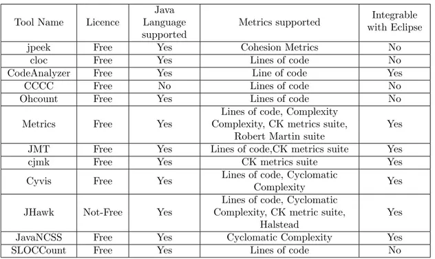
This research led to a few different metric gathering tools that can gather different kinds of metrics. Table 2shows all the tools we considered as a possibility for gathering metrics for software fault prediction.
Tool Name Licence
Java Language supported
Metrics supported with EclipseIntegrable
jpeek Free Yes Cohesion Metrics No
cloc Free Yes Lines of code No
CodeAnalyzer Free Yes Line of code Yes
CCCC Free No Lines of code No
Ohcount Free Yes Lines of code No
Metrics Free Yes
Lines of code, Complexity Complexity, CK metrics suite,
Robert Martin suite
Yes
JMT Free Yes Lines of code,CK metrics suite Yes
cjmk Free Yes CK metrics suite Yes
Cyvis Free Yes Lines of code, Cyclomatic
Complexity Yes
JHawk Not-Free Yes
Lines of code, Cyclomatic Complexity, CK metric suite,
Halstead
Yes
JavaNCSS Free Yes Cyclomatic Complexity Yes
SLOCCount Free Yes Lines of code No
Table 2: List of tools for metric gathering
We were able to find 9 tools that can collect Lines of Code, 4 tools that can collect Cyclomatic Complexity metrics, 4 tools that CK suite metrics, 1 tool that collect cohesion metrics, 1 tool that collects Robert Martin suite metrics and 1 tool that collects Halstead. With this results we
consider Lines of code, Cyclomatic Complexity and CK suite the easiest metrics to automatically gather through existing tools. A further reflection on metrics gathering was that it is very difficult to find tools that collect Halstead metrics. We found one tools that can collect Halstead metrics but it is not open source and thus violates one of the rules of tool selection.
This led to the decision to not use Halstead metrics in the fault prediction process. On the other hand, the considerable number of tools available for collecting traditional metrics such as Lines of code, McCabe cyclomatic complexity, and CK suite metrics together with the description of such metrics as good predictors in literature [5] reinforced our idea of using these metrics to predict faulty modules in our fault prediction tool.
A tool that proved to be of great help in this study is the Metrics 1.3.10 Eclipse plug-in. This is a tool easy to use and gathers different kinds of metrics. Moreover, Metrics is an open source tool, written in Java with the same nature (plug-in) tool we intended to develop. These are the reasons that led us to the decision of using this tool as the foundation to build our new tool upon. In order to reflect our finding on the easiest metrics to collect, we modified the Metrics source code to extract only Lines of code, McCabe’s cyclomatic complexity, and from the CK metrics suite: Weighted methods per class, Depth of inheritance tree, Number of classes, Direct class coupling, Lack of cohesion of methods. These metrics are used as the basis of prediction in our plug-in and as the basis for the prediction methods evaluation.
6
A Software Fault Prediction Tool
In this section, we describe our new Software Fault Prediction Tool for Eclipse IDE as a response to RQ 2. This is an Eclipse IDE plug-in called SFPPlugin that can be used to optimize quality assurance resources while still improving the quality of the software by predicting faulty modules in the projects.
6.1
SFPPlugin Components
The purpose of this plug-in is to predict the modules that have a high probability of containing faults in a specific project. To make this happen, we need a few components as described in Section 2.1 and clearly depicted in Figure 2. The main parts are training data (historic metrics and historic fault data), new metrics (calculated from the source code) and the prediction method. During the development of the SFPPlugin, we have modified the code of an existing metric gathering Eclipse plug-in: Metrics 1.3.10 to add the prediction capability. Metrics 1.3.10 measures the source code attributes in the form of metrics. This tool allows the gathering of a lot of metrics and in different levels of project hierarchy (project, package, class, method). For the purpose of our implementation, we extracted only the metrics that are relevant to us (LOC, McCabe Complexity, CK suite) at the level of class metrics.
These metrics make for the new metrics part of the prediction process. Another input necessary for the prediction is the training data. These data should be recorded by the tool users in an Attribute-Relation files (.arff) file that should contain metrics from the previous versions of the software matched with bug reports from these versions. This file will contain the description of the instances and their attributes used for the prediction. All the attributes present in this file are described in Table3.
Attribute Description
loc Lines of code metric
mccabe McCabe cyclomatic complexity metric
wmc Weighted methods per class metric
dit Depth of inheritance tree metric
noc Number of classes metric
dcc Direct class coupling metric
lcom Lack of cohesion of methods metric
class Prediction class (true for faulty modules and false for non-faulty ones)
Table 3: Arff attribute description
The training data is used to train a Naive Bayes predictor and a Logistic Regression predictor. For the implementation and the evaluation of the predictors, we have integrated WEKA API into the SFPPlugin. The trained predictors are then used to predict new instances using metrics gathered from the source code. The results of the predictions are displayed in a new view. Figure4 is an overview of the flow graph SFPPlugin and it is a more elaborate version of the graph in Figure2adapted to our specific tool.
Figure 4: SFPPlugin flow graph
6.2
SFPPlugin Users Perspective
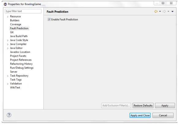
From the users perspective, the plug-in is easy to use and understand. A first prerequisite inherited from the Metrics 1.3.10 plug-in is that the project needs to be opened in an Eclipse perspective that shows Java resources as source folders, that can be Java or Java Browsing perspectives. The plug-in needs to be firstly enabled. By right-clicking on the project, the user needs to open the properties options for the project. The Fault Prediction properties interface will look like as in Figure5. The user needs to check the Enable Fault Prediction check box.
Figure 5: Enable Fault Prediction
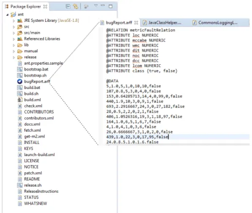
Next, the user needs to add the training data to the project. The training data is entered in a .arff file. Before the prediction, the user needs to save the Arff file in the root of the project and the file needs to be constructed accnording to the format shown in Figure6. The attributes of the instances are described in Table3and under the @Data section, the user needs to type the metrics and the fault information of the previous versions of the software. At this point, the user has to rebuild the project as a way of allowing the plug-in to read the fault information file just added.
Figure 6: Training data
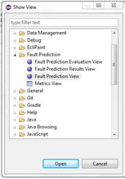
Now everything is set up and ready for conditioning fault prediction activities. Under the Eclipse views in Figure7, the user can select Fault Prediction View. The Fault Prediction view looks like in Figure8. All the metrics used for the prediction of fault-proneness of the classes are listed in this view by class files. These are the metrics calculated from the source code of the current version of the project. To see the predictions made for each entry of the list, the user must select the button on the top right of the view. This button opens a new view shown in Figure9, very similar to the first one, but now it includes the results of the prediction for the Naive Bayes and the Logistic Regression predictors. The user can see the predictions for all the class files and for both the predictors in one view. A class is labeled as“fault-prone” if the predictor concluded that it may be possible to be a fault in this class according to historic data and to source code metrics or it is labeled as “non-fault-prone” otherwise. The user can use this information to manage his quality assurance resources in a more efficient way.
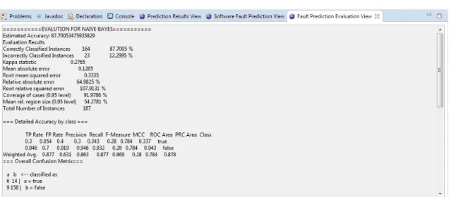
The results provided by the predictors will be different from one another. As will be demon-strated later in the Section7, the performance of the predictors differs from dataset to dataset. The decision of which predictions is better to use cannot be a personal preference of the project manager. To ease the choice and to provide further insight on how the predictors are performing on the users dataset, we also implemented a simple evaluation view. On the top right of the Prediction Results View, the user can select the Evaluate Prediction button and a view similar to the one in Figure10will appear. This view is really simple and only prints out basic performance information provided by WEKA after performing a 10-fold cross-validation on the training data provided by the user. The view does not involve any kind of interpretation of the results. The user is expected to draw his own conclusions.
However, this study also includes a performance evaluation of the Naive Bayes and Logistic Regression predictors in Section 7 on different kinds of open source datasets. This evaluation is followed by a discussion that draws general conclusions of which of the predictors has the best performance based on the datasets considered in this study.
Figure 7: Show Fault Prediction View
Figure 9: Fault Prediction Results View
Figure 10: Fault Prediction Evaluation View
A step by step description of how a user can interact with the SFPPlugin is shown below: 1. Open Java Perspective;
2. Enable Fault Prediction;
3. Add the training data in format .arff to the root of the project; 4. Rebuild Project;
5. Open Software Fault Prediction view; 6. Select the project;
7. Wait until all the metrics are calculated; 8. Click on the prediction button;
9. The prediction can be seen in the Prediction Results view; 10. Click the Evaluation button;
11. Evaluation for both methods using the provided dataset can be seen in the Evaluation view.
6.3
SFPPlugin Advantages
We believe that this plug-in is a great addition to the developers’ toolbox in their day-to-day work. It will increase the developer’s confidence and efficiency while coding and testing by directing their attention to the fault-prone modules. The fault prediction problem is complex and greatly depends on many factors that are sometimes impossible to predict during the development of such tools, like the balance of the data or the properties of the code. These factors affect the performance of different predictors in different ways. SFPPlugin uses more than one predictor for the prediction of the same data providing this way a degree of flexibility on different kind of data. The users of the SFPPlugin can choose to which of the prediction to take into account based on the evaluation of both predictors. Furthermore, since SFPPlugin is using WEKA API it can be very easy to add new prediction methods and evaluation measurements in the later versions of the tool. We are opening the source code for the SFPPlugin3 in hope that it can help further studies in this field.
Contributions are always welcomed to improve or add new features to this tool.
7
Prediction Method Evaluation Results
The objective here is to show the difference in performance between the fault prediction methods Naive Bayes and Logistic Regression based on the tool we created. This section will also serve as a response to RQ 3. The classifiers are evaluated in four open source projects: Tomcat, Ivy, Ant, Log4J. The metrics and bug reports for these projects are imported from the Metrics Repository 0.2.2 contributed by Jureczko [35]. The data collected for each dataset and the distribution of the data between faulty classes and non-faulty ones are depicted in Table4. Metrics Repository 0.2.2 contained a few versions of the projects. More specifically, it contained 1 version for Tomcat, 3 versions for Ivy, 5 versions for Ant, and 3 versions for Log4J. The amount of data between the different versions of the software varies from 122 records for the smallest dataset (Log4J v1.1) to 1162 for the biggest one (Tomcat v6.0.389418). For each dataset, we have combined the data of all available versions to form a bigger dataset. This is in hope to get an insight on how the classifiers perform in bigger datasets and to conclude if its better for the project manager to combine data from different versions or just the last version.
The data distribution includes datasets with imbalanced data such as Tomcat (v6.0.389418), Ivy (v1.4 & v2.0), Ant (all versions), and datasets with more balanced data Ivy (v1.1) and Log4J (all versions). It is important to mention that we are aware of the problems that come during evaluation based on imbalanced data [36]. However, the evaluation of the classifiers in this study is focusing on the performance of these classifiers in real datasets used by companies that will use SFPPlugin. This data may be very well imbalanced or balanced depending on different projects. One of the reasons why we selected datasets with different distribution is so that we can represent both situations.
The methods are evaluated using the SFPPlugin implemented in the study. The tool uses WEKA API and 10-fold cross-validation. We have run the tool one time for each of the datasets exported from the Metrics Repository. Each dataset is divided into 10 segments, 9 of them are used as training sets and the last one is used as a testing set. The results gathered from each run are gathered and organized in the following subsections.
Total Faulty Not-Faulty Faulty Data Rate
Tomcat v6.0.389418 1162 77 1085 6.62% Ivy v1.1 135 63 72 46.6% Ivy v1.4 321 16 305 4.98% Ivy v2.0 477 40 437 8.38% Ivy All 933 119 814 12.75% Ant v1.3 187 20 167 10.69% Ant v1.4 295 40 255 13.56% Ant v1.5 401 32 369 7.89% Ant v1.6 523 91 432 17.29% Ant v1.7 766 115 651 15.01% Ant All 2142 298 1844 13.91% Log4J v1.0 153 34 119 22.23% Log4J v1.1 122 37 85 30.32% Log4J v1.2 282 189 93 37.03% Log4J All 557 260 197 46.67%
Table 4: Data distribution
7.1
Incorrectly classified instances
The first measure of the evaluation is the percentage of incorrectly classified instances for both classifiers, and it is represented in Table 5. The incorrectly identified instances are both faulty instances incorrectly classified as non-faulty-prone and non-faulty instances incorrectly classified
Naive Bayes Logistic Regression Tomcat v6.0.389418 10,499% 6,626% Ivy v1.1 35,555% 29,629% Ivy v1.4 8,411% 5,296% Ivy v2.0 10,691% 8,805% Ivy All 14,898% 12,754% Ant v1.3 12,299% 10,695% Ant v1.4 24,905% 15,849% Ant v1.5 9,226% 8,728% Ant v1.6 17,017% 16,826% Ant v1.7 12,663% 11,357% Ant All 14,052% 13,071% Log4J v1.0 15,032% 14,379% Log4J v1.1 18,852% 13,934% Log4J v1.2 38,297% 24,113% Log4J All 32,316% 28,545%
Table 5: Incorrectly classified instances
as faulty-prone. A quick glance at the table shows that Naive Bayes has a higher percentage of incorrectly classified instances on all the evaluated datasets. The difference between the classifiers goes as high as 9,056%.
7.2
Confusion Matrix Rates
Table 6is a representation in terms of rate of the confusion matrix for each project. • TP - True Positive is the rate of instances that are correctly identified as faulty;
• FP - False Positive is the rate of the instances that are incorrectly identified as fault-prone. That is non-faulty modules classified as fault-prone;
• TN - True Negative is the rate of instances that are correctly identified as non-fault-prone; • FN - False Negative is the rate of instances that are incorrectly identified as non-fault-prone.
That is faulty modules that are classified as non-fault-prone.
This table is a good representation of how each predictor has labeled each instance and the rate of the correctness of each label. Hence, this table is a great source of information for many other evaluation measurements.
The main objective of the fault prediction process is to minimize the quality assurance effort and costs by orienting the tests to more fault-prone modules. Although this is true, the predictions are far from perfect and always include a percentage of incorrectness as clearly demonstrated in Table5. However, this percentage does not provide enough information for the classifier evaluation. The cost of classifying a faulty module as non-fault-prone one is different from the cost of classifying a non-faulty module as a fault-prone one. The later is mostly a matter of increased resource cost since the project manager will instruct to test this module thoroughly given that according to the prediction it may have some faults, even though it does not contain any. This kind of errors will not affect the final quality of the product but are critical in projects with budget constraints. On the other hand, classifying a faulty module as non-fault-prone may risk the final quality of the product. The mislabeled module may not be tested thoroughly and the faults may be detected later in the process or even pass undetected until the user encounters them. The cost of such scenarios is huge, especially in a safety critical system.
As can be seen, a prediction method with a low FN is very important in the fault prediction problem. From the data gathered, Naive Bayes had the lowest FN rates in most of the datasets like
Tomcat v6.0.389418, Ivy v1.4, Ivy v2.0, Ivy All, Ant v1.3, Ant v1.4, Ant v1.5, Ant v1.6, Ant v1.7, Ant All, and Log4J v1.1. Logistic regression had the lowest FN rates in fewer datasets like Ivy v1.1, Log5J v1.2, and Log4J All. Log4J v1.0 had the same FN rates for both prediction methods, labeling half of the faulty modules as non-fault-prone. Naive Bayes is also performing better in the True Positive (TP) category, meaning that Naive Bayes is correctly detecting a rate of faulty instances. It presents better rates is 9 out of 15 datasets including Ivy v1.4, Ivy v2.0, Ivy All, Ant v1.3, Ant v1.4, Ant v1.4, Ant v1.5, Ant v1.7, and Ant All. Logistic Regression has better True Positive rates in only 5 out of 15 datasets including Tomcat v6.0.389418, Ivy v1.1, Log4J v1.1, Log5J v1.2, and Log4J All. The dataset Log4J v1.0 had the same TP rates for both classifiers.
Dissipate this, Logistic Regression has better rates in the False Positive (FP) category present-ing lower values comparpresent-ing to Naive Bayes is 11 out of 15 datasets includpresent-ing Tomcat v6.0.389418, Ivy v1.4, Ivy v2.0, Ivy All, Ant v1.3, Ant v1.4, Ant v1.5, Ant v1.6, Ant v1.7, Ant All, and Log4J v1.0. Logistic Regression has also better rates in the True Negative (TN) category with lower values compared to Naive Bayes in 13 out of 15 datasets including Ivy v1.4, Ivy v2.0, Ivy All, Ant v1.3, Ant v1.4, Ant v1.5, Ant v1.6, Ant v1.7, Ant All, Log4J v1.0, Log4J v1.1, Log4J v1.2, and Log4J all.
It is also important to notice that the TP rates and the FN rate for datasets Ant v1.4 and Ant v1.5 using the Logistic Regression fault prediction method are equal to 0 and 1 respectively. This means that all the faulty modules are classified as non-fault-prone and just a few of the non-faulty modules are classified as fault-prone.
Naive Bayes Logistic Regression
TP FP TN FN TP FP TN FN Tomcat v6.0.389418 0,247 0,059 0,941 0,753 0,078 0,006 0,994 0,922 Ivy v1.1 0,349 0,097 0,903 0,651 0,571 0,181 0,819 0,429 Ivy v1.4 0,125 0,043 0,957 0,875 0,063 0,007 0,993 0,938 Ivy v2.0 0,350 0,057 0,943 0,650 0,125 0,016 0,984 0,875 Ivy All 0,185 0,052 0,948 0,815 0,067 0,010 0,990 0,933 Ant v1.3 0,300 0,054 0,946 0,700 0,200 0,024 0,976 0,800 Ant v1.4 0,475 0,200 0,800 0,525 0,000 0,009 0,991 1,000 Ant v1.5 0,375 0,046 0,954 0,625 0,000 0,008 0,992 1,000 Ant v1.6 0,297 0,058 0,942 0,703 0,242 0,044 0,956 0,758 Ant v1.7 0,452 0,052 0,948 0,548 0,365 0,022 0,978 0,635 Ant All 0,305 0,051 0,949 0,695 0,181 0,020 0,980 0,819 Log4J v1.0 0,500 0,050 0,950 0,500 0,500 0,042 0,958 0,500 Log4J v1.1 0,541 0,071 0,929 0,459 0,595 0,024 0,976 0,405 Log4J v1.2 0,460 0,065 0,935 0,540 0,825 0,376 0,624 0,175 Log4J All 0,377 0,061 0,939 0,623 0,558 0,148 0,852 0,442
Table 6: Classification result table
7.3
Precision Rates
Table7 represents the Precision rates for both classifiers for the predictions made for both classes (fault-prone and non-fault-prone). It is calculated as the rate of correctly identified instances in a specific class to the overall number of instances classified in that class as explained in the Section2.5.3.
For the dataset Tomcat v6.0.389418, Naive Bayes predicted 83 instances as fault-prone, from which 19 are correctly predicted the other 64 instances are actually non-faulty instances classified as fault-prone. That means that the Precision of Naive Bayes in the dataset Tomcat v6.0.389418 for the fault-prone class is 0,229. The Logistic Regression, on the other hand, predicted 12 fault-prone modules, form which 6 are correctly predicted and the other 6 instances are incorrectly classified
Fault-Prone Non-Fault-Prone
Naive Bayes Logistic Regression Naive Bayes Logistic regression
Tomcat v6.0.389418 0,229 0,500 0,946 0,938 Ivy v1.1 0,759 0,613 0,735 0,686 Ivy v1.4 0,133 0,333 0,954 0,953 Ivy v2.0 0,359 0,417 0,941 0,925 Ivy All 0,344 0,500 0,888 0,879 Ant v1.3 0,400 0,500 0,919 0,911 Ant v1.4 0,297 0,000 0,896 0,848 Ant v1.5 0,414 0,000 0,946 0,920 Ant v1.6 0,519 0,537 0,864 0,857 Ant v1.7 0,605 0,750 0,907 0,897 Ant All 0,492 0,600 0,894 0,881 Log4J v1.0 0,739 0,773 0,869 0,870 Log4J v1.1 0,769 0,917 0,823 0,847 Log4J v1.2 0,935 0,817 0,460 0,637 Log4J All 0,845 0,767 0,633 0,688
Table 7: Precision result table
as fault-prone. From this data, the Precision of Logistic Regression for the fault-prone class in the dataset Tomcat v6.0.389418 is 0.5.
The aim of a good predictor is to have as high of a Precision as possible in order to know that most of the instances classified in a specific class are true to that class. From the measurements gathered on all the datasets, the Logistic Regression classifier has the highest Precision for the fault-prone class in most datasets like Tomcat v6.0.389418, Ivy v1.4, Ivy v2.0, Ivy All, Ant v1.3, Ant v1.6, Ant v1.7, Ant All, Log4J v1.0, and Log4J v1.1. Naive Bayes, in contrast, presents higher Precision for the fault-prone class in fewer datasets like Ivy v1.1, Ant v1.4, Ant v1.5, Log4J v1.2, and Log4J All. Notice that the Precision of Logistic regression for the fault-prone class for the dataset Ant v1.4 and Ant v1.5 is 0 since in these datasets, Logistic regression did not classify correctly any of the faulty modules.
At the same time, the roles are inverted in the non-fault-prone class where Naive Bayes is the one that presents the higher Precision in most of the datasets like Tomcat v6.0.389418, Ivy v1.1, Ivy v2.0, Ivy All, Ant v1.3, Ant v1.4, Ant v1.5, Ant v1.6, Ant v1.7, Ant All. Logistic regression has the highest Precision for the non-faulty-prone class in all the Log4J datasets. Ivy v1.4 presents almost the same Precision rates for both classifiers with a slight advantage for the Naive Bayes.
However, the measurements of Precision does not tell the full story regarding performance as a classifier can present a higher rate of Precision because the overall number of instances classified in a specific class is low. An excellent example of this situation is the one depicted in the second paragraph of this subsection for the Tomcat dataset. Naive Bayes actually correctly classified a higher number of instances in faulty class and at the same time, it incorrectly classified a higher number of faulty instances and thus lowering the rate of Precision. Again, classifying non-faulty modules as fault-prone increases the cost of quality assurance but does not affect the overall quality of the software. While Logistic Regression has a higher Precision rate because it predicted a low number of instances as faulty overall. This means that a lot of the true faulty instances are classified as faulty and this is clearly depicted for the lower Precision rates in the non-fault-prone class. Depending on the application, whether a safety critical application or a budget constrained, one kind of error can be preferable to the other.
Overall, the Precision rates for the fault-prone class in most of the datasets are low and rarely reaching the 0.5 rate. The datasets presenting better Precision rates for both classifiers, rates over 0.6, are the more balanced datasets. This is expected since in the more imbalanced datasets the classifiers will tend to overclassify instances in the more dominant class, in this case, the