2019; 5(1): 37-49
Published by the Scandinavian Society for Person-Oriented Research Freely available at http://www.person-research.org
DOI: 10.17505/jpor.2019.04
A hybrid approach to regime shift detection
Alexander von Eye
1,Wolfgang Wiedermann
2, and Stefan von Weber
31
Michigan State University
2
University of Missouri, Columbia
3
University of Furtwangen, Germany
Correspondence concerning this article can be addressed to Alexander von Eye, Michigan State University, Department of Psychology, East Lansing, MI, 48824; e-mail: voneye@msu.edu
To cite this article: von Eye, A., Wiedermann, W., & von Weber, S. (2019). A hybrid approach to regime shift detection. Journal for
Person-Oriented Research, 5(1), 37-49. DOI: 10.17505/jpor.2019.04
Abstract
In this article, we propose a method for the analysis of regime shifts in frequency data. This method identifies those points in the develop- ment of a process for which deviations are most extreme. Based on a statistical model, functions are estimated that describe the process. This description can represent either the entire series of scores or the series before and after a shift point. The shift point can be either given a priori or estimated from the data. The method is hybrid in that it first uses standard models for the estimation of parameters of the process that is examined and then, in a second step, elements of Configural Frequency Analysis. Uni- and multivariate versions of the method are proposed. In data examples, road traffic data from California and Germany are analyzed before and after particular shift points. Extensions of the proposed method are discussed.
Keywords: regime shift; multivariate; Configural Frequency Analysis; log-linear Modeling; linear models
A regime is defined as a characteristic behavior of a sy- stem that is stable over time. Examples of regimes often considered time-stable include personality in humans and the climate of the earth. When these characteristics change to the extent that it is statistically detectable, one observes a regime shift. Examples of regime shifts include changes in personality that are caused by traumatic events such as accidents, and changes in climate that are caused by global warming.
The statistical analysis of regime shift phenomena can focus on just any parameter that is used to describe the behavior of a system over time. These include, for instance, means, trend parameters, covariance structures, or higher order moments. Overview articles that summarize such methods have been published by, for example, Liu, Wan, and Gu (2016) and Rodionov (2005). The latter author classifies existing methods for the detection of regime shift into the following eight categories:
1. Non-parametric methods. Among other tests, this category includes the non-parametric Mann-Whitney U-test. It can also be used for the detection of changes in means (for a discussion of tests of changes in means, see Wieder-mann and Alexandrowicz, 2007).
2. Parametric methods. The best known of these meth-ods is the t-test. It requires the assumption that the data are normally distributed and homoscedastic. It allows one to identify shifts in means over time.
3. Curve-fitting methods. These methods capture the curvature of a series of measures instead of the mean. A regime shift in curvature occurs when the shape parameters of a curve cease to describe the curve after a particular point in time.
4. Bayesian analysis. Bayesian methods can also be used to estimate parameters of time series. They differ from the methods listed under 1 – 3, in that researchers need to specify prior distributions. With respect to these distribu-tions, a posteriori distributions are estimated. Uncertainty estimates of change points and parameters after the change can be calculated.
5. Cumulative sum methods. These methods focus on cumulative deviations from a mean. After a regime shift, cumulative deviations increase when the mean from before the shift is still used as reference.
6. Regression-based methods. Most popular are linear, curvilinear, and autoregression methods, including vector- autoregression models (originally proposed by Granger,
1969; cf. Koller, Carstensen, Wiedermann, & von Eye, 2016; Molenaar, & Lo, 2016; Rovine, & Walls, 2006). These methods are relatives of the methods listed under 3, in that regime shifts materialize in change in parameters that is observable after a particular point in time.
7. Sequential methods. This group includes, for instance, runs tests or Wald statistics. These are methods that exam-ine the sequencing of events or the magnitude of deviations that is considered admissible over time.
Here, we add an eighth group of methods, one that has received considerable attention in recent years.
8. Methods based on second- and higher-order statistics. This group includes structural and dynamic models as they are discussed, for instance, by Hamaker, Grasman, and Kamphuis (2010). Here again, regime shifts are indicated by changes that invalidate the originally estimated para- meters after a particular point in time.
All of the methods in this list (cf. the list provided by Liu et al., 2016) share two characteristics. First, they can be used to identify an a priori unknown point in time from which on the regime shift can be considered established, but they can also be used to estimate separate models for before and after hypothesized points in time at which the regime changes (henceforth called shift point). Most of these methods can be used for the analysis of one or more shift points in time. Second, these methods use information from the entire series of data points, and they allow one to talk about the series of data points as a whole, the series before, and the series after the presumed shift point.
In the present article, we propose a configural method that shares both characteristics. However, in addition, this method also allows the researcher to make statements about individual points in time, before and after the estimated or hypothesized shift point. The proposed method is configu-ral in that it uses elements of Configuconfigu-ral Frequency Analy-sis (CFA; Lienert, 1969; von Eye, 2002; von Eye, & Gutiérrez Peña, 2004). In contrast to known methods of CFA, however, the proposed method does not use log-linear models or a priori probabilities to estimate expected values, but assumptions or results from applications of other statis-tical methods about trends that might exist for the entire series or part of it. We call the proposed method regime shift CFA.
The remainder of this article is structured as follows. First, we provide a review of CFA and introduce univariate regime shift CFA. We then present a data example in which we combine regime shift CFA with regression-type meth-ods (Group 5 of the above list). In this example, we exam-ine traffic data that describe accident rates before and after the implementation of a seat belt law in California. In this example, regression methods are used to estimate a trend, and CFA is used to identify local deviations from this trend. This is followed by an introduction of multivariate regime shift CFA. This method allows one to simultaneously con-sider multiple series of data in the same analysis, with re-spect to the same shift point. The method is exemplified using autobahn traffic death data from Germany.
An overview of CFA
CFA is a method that allows one to identify local, that is, cell-wise deviations from a model that is used to describe the frequency distribution in a cross-classification of two or more categorical variables. In most cases, the distribution in such tables is multinomial or product-multinomial. Suppose that the cross-classification is spanned by d varia-bles. Variable i has ci categories, with i = 1, …, d, and the
cells are numbered 1, 2,… r,…, R, where 𝑅 = ∏ 𝑐𝑖
𝑑
𝑖=1
is the total number of cells of the cross-classification. Let mr be the frequency of observations in cell r. When samp-
ling is multinomial, Mr is binomially distributed with
𝑃(𝑀𝑟 = 𝑚1, . . . , 𝑀𝑟= 𝑚𝑟│𝑁, π1, . . . , π𝑅) = 𝑁! 𝑚1!. . . 𝑚𝑅! ∑ 𝑅 𝑖=1 π𝑟 𝑚𝑟,
where the Mi indicate the configurations (cells), with i =
1, …, R, the πi are the binomial cell probabilities, Σπi = 1,
and Σmr = N the sample size. In both cases, the summation
goes over all cells of the cross-classification (cf. von Eye, & Gutiérrez-Peña, 2004). Now, let 𝑚𝑟′ be the expected frequency of Cell r, under some base model. Then, the null hypothesis, 𝐻0: 𝐸[𝑚𝑟] = 𝑚𝑟′ is rejected either because the binomial probability for mr is
𝐵
𝑁,π𝑟(𝑀
𝑟− 1) ≥ 1 − α
that is, Cell r constitutes a CFA type, or because
𝐵
𝑁,π𝑟(𝑚
𝑟) ≤ α,
that is, Cell r constitutes a CFA antitype (for more detail, see von Eye, & Gutiérrez Peña, 2004; for more CFA tests, see von Eye, 2002). Evidently, CFA needs information to generate expected cell frequencies. In virtually all applica-tions, this information stems from two sources. The first source is the observed frequency distribution. The second source is given by the model that is used to estimate the expected cell frequencies (cf. von Eye, 2004). As was indi-cated above, most of the probability models used for CFA are log-linear models of the form log m = Xλ, where X is the design matrix and λ is the parameter vector. Sampling for these models is binomial or multinomial, and the models specify the effects considered in a particular CFA. Alternatively, a priori probabilities can be used.
CFA and regime shifting
In the present context, we propose a CFA model that dif-fers from the ones discussed in the literature thus far in one
major respect. Specifically, the model uses neither log- linear modeling nor a priori probabilities. Instead, a func-tion is specified that describes ordered data. This funcfunc-tion describes the data of either the entire series or a segment of this series. This function is used to estimate the expected frequencies of the series of observations. The CFA model that is proposed can be applied to both single and multiple variables that are observed over time.
Thus far, almost all CFA models required that two or more variables be crossed. The only exception to this rule is constituted by unidimensional CFA in which univariate time series were compared with expectations of stability (see Ch. 9.7 in von Eye, 2002); that is, the model used was an intercept-only model. In the following sections, we de-scribe regime shift CFA from an algorithmic perspective.
Let 𝑀𝑟= 𝑓(𝑥) be the function that describes the rela-tion of the observed series of frequencies to time. There are no limits to the selection of this function, except those that are natural for frequency data. For example, functions must be avoided that estimate negative frequencies, frequencies larger than the sample size, frequencies for scores outside the range of the scale, or functions that impose characteris-tics on the scale of X that are not compatible with the scale level of X.
Under most conditions, for example in unidimensional CFA, the parameters of these functions are estimated for the entire range of X. In contrast, in regime shift CFA, functions are estimated just for the range that ends (and begins) at the shift point. In other words, a function is esti-mated for a segment of the data. For the following segment, a different function may apply, or no function is estimated at all. Therefore, the functions that we use in regime shift CFA can be given by 𝑀𝑟= 𝑓(𝑥)│𝑟 ≤ 𝑠, where s is the shift point on X.
For the following considerations, we require that this function describe the data well, all the way to the shift point, s. This point can either be estimated based on the data (cf. Zhang & Siegmund, 2007; von Eye, & Schuster, 1998), or it is given based on theory, or by some event. The CFA- specific element of regime shift detection is that the func-tion does not necessarily describe the data well after the regime shift point. That is, the function that describes the data well up until s might fail to represent the data after s, and CFA types or antitypes may emerge after s. These are defined with respect to the function that describes the sec-tion of the data before s. They indicate where exactly in the series of observations the function from before s does not apply any more, and the direction in which the deviation goes (this is the definition of CFA types and antitypes). In the following section, we present a data example, from traffic statistics.
Data example
In this section, we present a data example from traffic statistics. This example may seem a little radical. We
re-frain, however, from taking sides or from proposing any changes in traffic laws. We just discuss data.
Data Example: Brock Yates’ death rates and seat belt statistics. In 2001, Yates published, in the magazine Car and Driver, an article about death rates in car accidents before and after seat belts were required in California. The author concluded that, after seat belts were required in California, “… the death rates should have trended down-ward following the seat belt law implemented in 1986. But, in fact, the rate trended upward ...” (Yates, 2001, p. 3). The author also reports that, in Tennessee and in Washington DC, death rates went upwards as well.
In the present context, we ask the following, related question. Given the downward trend in traffic accident death rates in California that was observed before 1986, did the enactment of the seat belt law result in a regime shift such that this trend was broken? More specifically, one would have hoped that the introduction of seat belts would have broken the trend such that it accelerated or, in other words, that the reduction in traffic accident deaths acceler-ated.
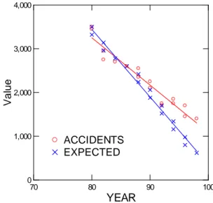
To answer this question, we apply regime shift CFA in tandem with ordinary least squares (OLS) regression analy-sis. We proceed in three steps. First, we estimate a function that describes the death rates data before 1986. Then, we ask whether the same function validly describes the data after 1986. Third, we apply the estimates from this function, and ask where, in the years after 1986, deviations were most pronounced and in which direction they went. For the first step, we apply simple, linear regression methods. In the second step, we apply piecewise linear regression methods. In the third step, we apply regime shift CFA. Figure 1 displays the data. The smoothed curves are linear OLS approximations for the observed and expected fre-quencies (to be explained later).
Figure 1. Observed and expected accident frequencies for California from 1980 through 1998 (observed frequencies from Yates, 2001). EXPECTED ACCIDENTS 70 80 90 100
YEAR
0 1,000 2,000 3,000 4,000 V a lu eFigure 1 shows that the number of deadly traffic acci-dents in California decreased steadily over the observation period, with no visible acceleration or deceleration after 1986, the year in which seat belts were made mandatory. We now ask whether the same linear regression describes the data well over the entire observation period, or whether the period before 1986 requires a separate regression line. To answer the first question, we estimate a simple linear regression model in which we regress accident numbers on year. Table 1 summarizes results.
The results in Table 1 show clearly that a single regres-sion line would be sufficient to describe the development of deadly traffic accidents in California for the observation period from 1980 through 1998. The coefficient of deter-mination (R2) is 0.940, an exceptionally large value. Still, the visual inspection of Figure 1 and the residual plot in Figure 2 suggest that the regression residuals increase over the range of predicted scores. Therefore, we now estimate two piecewise linear regression models (see von Eye, & Schuster, 1998). These models split the regression line at a particular point on X in two, and separate parameters are estimated for the sections before and after this point. The point can be either given by the data analyst or estimated, thus optimizing fit.
Figure 2. Residual plot of the OLS regression in Figure 1.
In the first run, we set 1986 as the shift point. Piecewise regression results are summarized in Table 2. Regression is linear and estimation was performed under least squares. In the Appendix, we present the SYSTAT code for this run.
Table 1. Regressing Number of accidents on Year. Regression
Coefficients Coefficient Standard Error
Standardized
Coefficient t p-value
Constant 11,914.767 629.667 - - -
Year -108.301 7.065 -0.970 -15.329 <0.001
Table 2. Piecewise regression of Number of accidents on Year, with 1986 set as shift point.
Parameter Estimate Asymptotic Standard Error (ASE) Parameter/ ASE
Wald 95% Confidence Interval
Lower Upper
Intercept 14,157.816 1,944.127 7.282 9,988.078 18,327.553
Year before 1986 -135.410 23.331 -5.804 -185.451 -85.370
Year after 1986 39.687 32.603 1.217 -30.240 109.615
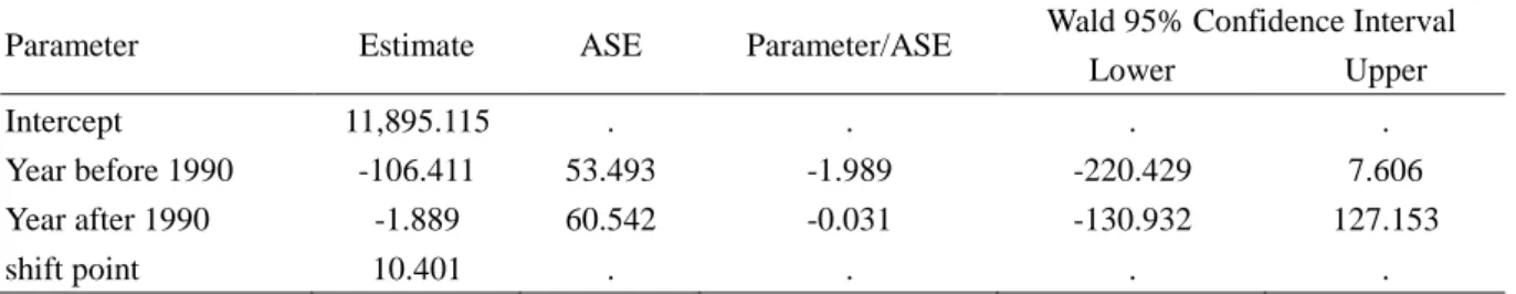
Table 3. Piecewise regression of Number of accidents on Year; shift point is estimated.
Parameter Estimate ASE Parameter/ASE Wald 95% Confidence Interval
Lower Upper
Intercept 11,895.115 . . . .
Year before 1990 -106.411 53.493 -1.989 -220.429 7.606
Year after 1990 -1.889 60.542 -0.031 -130.932 127.153
The results in Table 2 support the results from Table 1 and our conclusion from visual inspection of the data. The regression parameter for the time period after 1986 fails to be significant. This suggests that linear regression for the development of accidents after 1986 is no different than the regression before this point in time. The overall R2 for this model is 0.946, only minimally better than for the model of the entire data set.
One reason why the improvement is only minimal might be that drivers respond to the new seat belt law only after some adaptation period, that is, not immediately (enforcing the law several months after enacting it may have played a role; see Cohen & Einav, 2003). Therefore, we now re- estimate the piecewise regression model, but we estimate the possible shift point instead of setting it to 1986. Results of this run are summarized in Table 3, and the SYSTAT code appears in the Appendix. As in the first piecewise regression run, we opted for linear regression and least squares estimation.
The overall R2 for this model is 0.946 again, no better than for regression of the entire data set. In this model, the regression parameter for neither observation period is sig-nificant. The estimated shift point is 10.4. This corresponds to about Year 1991 (10.4 is after the tenth year in the ob-servation period, that is, after 1990), and points to a possi-bly long delay in drivers’ responses to the 1986 seat belt
law.
Considering the extremely high R2 values, one might be tempted to conclude that the introduction of the seat belt law in California had no effect on the development of deadly road accidents. If this is the conclusion, one won-ders how Yates would justify his statement that “the rate trended upward ...” (2001, p. 3). To illuminate this issue, we now apply configural regime shift analysis.
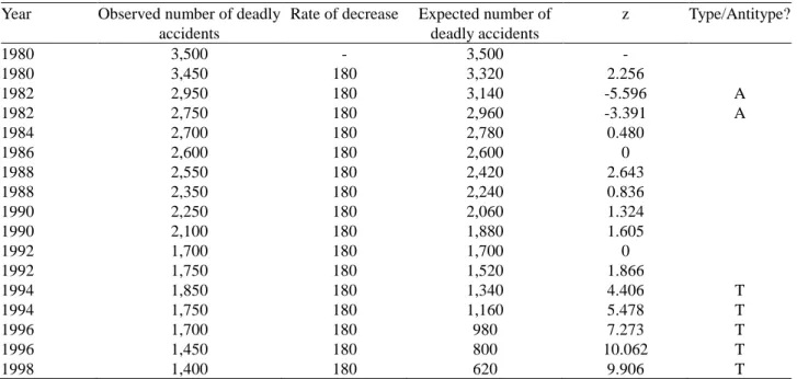
The question we strive to answer with regime switch CFA concerns the development of numbers of deadly traffic accidents before and after the seat belt law was enacted. If there is no regime shift, the decrease in death toll continues unchanged after 1986. Regime shift CFA was performed as follows. First, we calculated the average decrease from the data for the years 1980 through 1986. This number was 180. Using this number, we, then, calculated the expected num-ber of fatal road accidents for all observations, that is, for the entire series of frequencies, after 1980; and the z-scores for the differences between the observed and the expected numbers of deadly traffic accidents. A total of 17 compari-sons was made. The Bonferroni-protected significance threshold for the nominal α = 0.05 is, for 17 tests, 0.00294. The corresponding z-score is 2.7543. Every z > ± 2.7543 points to a CFA type or an antitype. Table 4 displays the results from regime shift CFA.
Table 4. Regime shift CFA of Yates’ traffic deaths data, assuming that the seat belt law did not change the development of the number of deadly traffic accidents.
Year Observed number of deadly accidents
Rate of decrease Expected number of deadly accidents z Type/Antitype? 1980 3,500 - 3,500 - 1980 3,450 180 3,320 2.256 1982 2,950 180 3,140 -5.596 A 1982 2,750 180 2,960 -3.391 A 1984 2,700 180 2,780 0.480 1986 2,600 180 2,600 0 1988 2,550 180 2,420 2.643 1988 2,350 180 2,240 0.836 1990 2,250 180 2,060 1.324 1990 2,100 180 1,880 1.605 1992 1,700 180 1,700 0 1992 1,750 180 1,520 1.866 1994 1,850 180 1,340 4.406 T 1994 1,750 180 1,160 5.478 T 1996 1,700 180 980 7.273 T 1996 1,450 180 800 10.062 T 1998 1,400 180 620 9.906 T
Table 4 shows traffic fatalities from 1980 through 1998, in raw numbers. The table shows that, from 1980 through 1986, there were only two significant deviations from ex-pectancy. In the year 1982, significantly fewer fatal road accidents were observed than expected, for both measures. Of central importance to the evaluation of Yates’ statement about the increase in the trend in number of deadly traffic accidents is the development of number of accidents after 1986. We can first note that, if Yates’ statement is applied to raw frequencies, it does not find support in the data. Every year, the raw number of deadly traffic accidents decreased. This is in contradiction to Yates’ statement, even if one interprets this statement as trend in development instead of trend in absolute numbers.
However, Table 4 suggests that this trend is not stable. In the years 1994, 1996, and 1998, significantly more deadly traffic accidents were observed than suggested from the trend from the years before the seat belt law. In addition, the deviation in 1996 is the strongest deviation from ex-pectancy in the entire table. Evidently, this counters the trend in development. It is outside the scope of this article to ask questions concerning the causes for this trend and the deviations from it.
Still, we note that, for the first 5 years after the law was enacted, the effect of the seat belt law on the number of deadly road accidents was, in California and for the obser-vation period, minimal at best. Over the years, the number of traffic victims did go down, simple linear regression models can capture this development, and regime shift CFA identified the observation points in time where deviations from the overall trend are most pronounced. The direction of these deviations supports Yates’ trend statement, in part.
Multivariate regime shift
In the following sections, we discuss and illustrate multi- variate regime shift CFA. Specifically, we consider the case in which two or more series of frequency scores are ana-lyzed that were created over the same observation span. In addition, we use the same shift point for both series of observations.1
For multivariate regime shift, we can estimate multivari-ate regression models of the form 𝑌 = 𝑋𝐵 + 𝐸 where Y is the n x s matrix of s series of n frequency scores, X is the design matrix, B is the vector of m + 1 regression parame-ters, and E is the n x s matrix of regression residuals. This model can be applied to the entire series, to the series be-fore the shift point, and to the series after the shift point.
1
Here and, as we assume, in most applications, the same shift point is implemented for the multiple observed series. However, there may be reasons why shift points differ over the multiple series.
The usual constraints apply. For example, n must be larger than s.
Similarly, when log-linear modeling is employed for the estimation of expected cell frequencies, the model log 𝑚 = 𝜆 + 𝜆𝑆+ 𝜆𝑅+ 𝜆𝑆𝑥𝑅 can be used, where m
indi-cates the model frequencies, R indiindi-cates the observation points and S indicates the series of scores. Assuming no time-related change of frequencies, the interaction term is omitted. Covariates and special contrasts can be incorpo-rated in this model.
Data Example
In the following section, we illustrate multivariate con-figural regime shift analysis using a real-world data set. The data, downloaded from the web site of the Deutscher Verkehrssicherheitsrat (2019), describe the development of fatal traffic accidents (D) and injuries in traffic accidents (I) on German highways (autobahns) from 1992 through 2017 (Y). For each year, the number of occurrences is reported. Table 8 below displays the year by type of event 26 × 2 frequency table. The table clearly suggests that the number of traffic deaths decreases over the observation period, and so does the number of injuries, but less evenly.
We analyze these data in four ways. First, we perform standard multivariate regression analysis of D and I on Y, the predictor. This analysis is used to answer the question whether there is a systematic, linear change in occurrence rates of fatal traffic accidents and injuries in traffic acci-dents over the observation period. Second, we perform piecewise regression separately for D and I. The year 2007 is used as shift point. The reason for the selection of this point is that, in 2007, the blood alcohol level was lowered in Germany above which driving under the influence is punishable. These two analyses are used to answer the questions of whether this new law changed the general trend to the better, that is, whether traffic deaths and inju-ries decreased in numbers even more than before, and whether there are deviations from these trends.
The two regression analyses are followed by one log-linear (Agresti, 2007; von Eye, & Mun, 2013) and one configural analysis (von Eye, 2002; von Eye, & Gutiérrez Peña, 2004). The log-linear analysis is performed to answer the question whether, in the 26 × 2 cross-tabulation of type of event and year, the independence model can be retained. The configural analysis is performed to identify those years in which particularly strong deviations are observed when a base model is used in which expected cell frequencies are estimated separately for the periods before and after the shift point, the year 2007.
Regression analyses. In the multivariate regression mod-el D and I were the dependent variables, and Y the inde-pendent variable. The F-tests for this model are given in Table 5. Table 5 shows that both dependent variables, D and I, are strongly dependent on Y. This suggests that,
over the observation period, systematic change occurs that can be captured by linear regression analysis. The adjusted squared multiple correlations (R2 = 0.943 for D and R2 = 0.675 for I) show that these relations are strong, and that they are slightly stronger for D than for I. The Wilks Lambda = 0.048 (F2, 23 = 229.881: p < 0.01)
indi-cates that the regression model, overall, explains 95.2% of the variance of the dependent measures.
Table 5. Multivariate regression with D and I as the de-pendent and Y the indede-pendent variables.
Source Type III SS df Mean Squares F p
DEATHS 1,640,001... 1 1,640,001... 414.634 <.001
Error 94,927.218 24 3,955.301
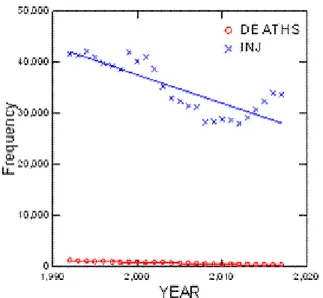
INJ 4.566E+008 1 4.566E+008 52.805 <.001 Error 2.075E+008 24 8,647,543... Figure 3 displays the regression slopes. The figure sug-gests that, for injuries, the shift point of 2007 may have led to a regime shift, but not for the development of traffic deaths on German autobahns.
Figure 3. Regression of Traffic Death and Injury Rates on Time.
Considering that accident counts come with rather small errors, we hypothesize that, maybe, even more variance can be explained by more detailed analysis. To explore this hypothesis, we first perform piecewise regressions sepa-rately on both dependent variables, D and I. As was ex-plained above, the shift point was set to the year 2007. Table 6 displays the estimated parameters for D.
Of the three parameters in Table 6, B0 is the constant of the model, B1 is the slope parameter for the period before 2007, and B2 is the slope parameter for the period after 2006. The table suggests that both slope parameters are significant. In addition, the model explains a large portion of the variance of D (mean-corrected R2 = 0.960, a slight improvement over the multivariate model). Figure 4 dis-plays the slopes of this piecewise regression run.
Figure 4. Piecewise regression of traffic Deaths (shift point is 2007).
Table 6. Piecewise regression for autobahn accident deaths (D; shift point is the year 2007).
Parameter Estimate Asymptotic standard error (ASE)
Parameter/A SE
Wald 95% Confidence Interval
Lower Upper
B0 80,622.293 5,171.307 15.590 69,924.629 91,319.957
B1 -39.889 2.585 -15.430 -45.237 -34.541
Figure 4 sheds more light on the results of the piecewise regression. For the period before the shift point, we observe a steady decline in fatal traffic accident rates on German autobahns. After the enactment of the new alcohol limit law, this decline seems to level off. Discrepancies between observed frequencies and the regression line are small throughout. Still, we conclude that, to do justice to the effects of the change in law, more detailed analysis may be needed.
Before performing this analysis, we examine the results for injuries in autobahn accidents. Table 7 presents the results of the corresponding piecewise regression analysis for I. As for D, the shift point was set to 2007 again.
Table 7 suggests that both of the parameters of interest are significant. The mean-corrected R2 is 0.813, a clear improvement over the multivariate model above. Although high, this value suggests that there may be variance that, in more detailed analyses, can be explained. Figure 5 displays the slopes of this piecewise regression run.
Figure 5. Piecewise regression of Injuries in traffic (shift point is 2007).
Figure 5 suggests that, for the period before the new driving under the influence law was enacted, there is a steady decline in injuries in autobahn traffic accidents. After that juncture, this trend is reversed. The number of injuries seems to increase.
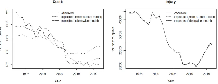
Log-linear and configural analyses. Considering that we here analyze frequency data, we can estimate log-linear models. Observed and expected frequencies for accident deaths and injuries are summarized in Figure 6. The first model is a base model that can be used for purposes of obtaining an overview and comparison. The model we estimate is the log-linear main effect model. Specifically, we estimate the model log 𝑚 𝜆 + 𝜆𝐷+ 𝜆𝐼, where m are
the model frequencies, and λD and λI are the model main effect parameters. Table 8 and Figure 6 display the ob-served and the expected cell frequencies of the 26 × 2 cross-tabulation of year and type of event.
The log-linear main effect model fails to describe the frequency distribution of the 26 × 2 cross-tabulation of year and type of event. We obtain the Pearson Chi-square of 1,076.279 (df = 25, p < 0.01) and the likelihood ratio chi-square of 1,115.364 (df = 25, p < 0.01). Based on these values, we reject the model and ask whether a regime shift at the year 2007 allows us to explain the data.
Configural analysis. We now perform a more detailed analysis of the cross-classification in Table 8. First, we estimate a log-linear main effect model that consists of two elements. Separate parameters will be estimated for the period that ends at the year 2006, and the period that begins in 2007. Considering that the piecewise regression runs resulted in improved model fit, we expect the two-part log-linear main effect models to result in smaller residuals than the one from the overall model in Table 8. The model we estimate is
log 𝑚 = 𝜆 + 𝜆𝑌𝑒𝑎𝑟<2007+ 𝜆𝐸𝑣𝑒𝑛𝑡 Ι 𝑌𝑒𝑎𝑟<2007
+ 𝜆𝑌𝑒𝑎𝑟>2006+ 𝜆𝐸𝑣𝑒𝑛𝑡 Ι 𝑌𝑒𝑎𝑟>2006,
Second, when these log-linear models still suggest sig-nificant model-data discrepancies, relations between year of observation and type of accident must exist. However, instead of modeling these relations, we perform a configu-ral analysis to identify the years with the biggest change and, thus, regime shift. Table 9 and Figure 6 display the results of the two-element log-linear model.
The two-element model with separate parameter estima-tion for the periods before 2007 and after 2006 does not describe the frequency distribution well either. There are large standardized residuals. Relations between year and type of accident must exist. We now ask where the dis-crepancies from the two-element base model and the data are largest and whether they display an interpretable pat-tern.
Table 9 will now be analyzed using configural frequency analysis (CFA; Lienert, & Krauth, 1975; von Eye, & Gutiérrez Peña, 2004). CFA allows one to identify those patterns that contradict a base model. Instead of consider-ing a base model simply rejected, these patterns are inter-preted with respect to the characteristics of the base model and a priori hypotheses (for more detail on CFA base mod-els and significance testing in CFA, see von Eye, 2004).
In the present example, the standardized residuals in the last two columns in Table 9 are examined with reference to the limits posed by a Holland-Copenhaver-protected sig-nificance threshold (Holland & Copenhaver, 1987). For a nominal significance threshold α, the protected threshold αi
is, for the ith out of r tests on the same sample,
α
i= 1
− (1− α )
1
where the tail probabilities of the individual tests are ar-ranged in ascending order. The Holland-Copenhaver pro-cedure is more powerful than the often-used Bonferroni procedure. In the present analysis, we select the nominal α = 0.05. The first protected threshold is α1 = 0.00197.
Inspecting the residuals in Table 9, we notice that they exhibit two interesting characteristics. First, not a single residual in the injuries list exceeds the protected limits (see also Figure 6, right panel). The base model can, therefore, be retained in the domain of injuries. Second, and in con-trast, there are extreme discrepancies in the fatal autobahn accident list.
Specifically, in the period before the new alcohol law, there are eight significant discrepancies. Four of these are located in the first half of this period, the other four in the second half. Interestingly, each of the first four constitutes a CFA type. That is, more cases were observed than expected. Each of the second four constitutes a CFA antitype. That is, fewer cases were observed than expected. We conclude that, in the space of autobahn accidents that are either fatal or result in person injuries, fatal injuries decrease in number more rapidly than expected under the assumption of inde-pendence of the first time period and type of event.
Looking at the development of type of event after en-actment of the new alcohol law, a similar picture emerges. There are six CFA types and antitypes. The first three of these are observed in the first half of this period, and the second three in the second half. As before, the first three discrepancies are all CFA types, and the second three are all CFA antitypes. After enactment of the new law, the number of deadly autobahn accidents thus first increased and then decreased faster than expected under the assumption of independence of the second time period and type of event.
From the perspective of regime shift analysis, this sug-gests that, under consideration of the main effects of the
observation points in time, there is no regime shift in auto-bahn accident injuries. In contrast, there is a regime shift in the development of fatal autobahn accident numbers. Spe-cifically, these numbers discontinue their smooth decline. Instead, the resume their development at a level signifi-cantly higher than expected, and then decline at a rate that is, toward the end of the observation period, more rapid than expected.
On first look, this result could be viewed as contradicting the data table and regression results above. However, differences between the models that were estimated in the analyses of the accident data can be used to explain the two sets of results. In the regression models, separate slopes are estimated for the two series of data that, in a least squares sense, minimize the differences between observed and expected accident frequencies (see Figures 4 and 5). Distortions and biases can occur, mostly because of the correlation between the two series of autobahn accidents. In the present log-linear main effect models, the expected frequencies are estimated such that the raw differences between the observed and the expected values are about the same, over the years and for each series of frequencies. This applies to both the sections before and after the shift point (see Table 9). Considering that the numbers of fatal autobahn accidents are smaller than the numbers of auto-bahn accidents with injuries, the same difference results in larger standardized deviates, as can be seen in Table 9.
This result is both model-specific and data-specific. This can be illustrated by simply dividing the numbers of severe injuries by 10. The resulting main effect models will still not fit, but after this transformation the raw differences between the observed and the expected cell frequencies are still about equal, but now the larger standardized residuals emerge in the column for injuries instead of the column for deaths.
Figure 6. Observed (solid lines) and expected frequencies of accident deaths and injuries based on log-linear main effects (dotted lines) and piecewise models (dashed lines). The shift point for the piecewise models is 2007.
Table 7. Piecewise regression for autobahn accident injuries (I; shift point is the year 2007).
Parameter Estimate ASE Parameter/ASE
Wald 95% Confidence Interval Lower Upper B0 1,874,627... 220,119.400 8.516 1,419,275... 2,329,978 B1 -918.789 110.038 -8.350 -1,146.420 -691.158 B2 1,007.697 256.741 3.925 476.589 1,538.806
Table 8. Observed and expected cell frequencies of the log-linear main effect model of the 26 x 2 cross-tabulation of year and type of event.
YEAR
Event Event Event
Death Injury Death Injury Death Injury
Observed Expected Standardized Residuals
1992 1,201 41,586 840.909 41,946.091 12.418 -1.758 1993 1,109 41,322 833.912 41,597.088 9.526 -1.349 1994 1,105 42,142 849.949 42,397.051 8.748 -1.239 1995 978 41,010 825.206 41,162.794 5.319 -0.753 1996 1,020 39,796 802.172 40,013.828 7.691 -1.089 1997 933 39,332 791.343 39,473.657 5.036 -0.713 1998 803 38,619 774.775 38,647.225 1.014 -0.144 1999 911 41,910 841.577 41,979.423 2.393 -0.339 2000 907 40,198 807.852 40,297.148 3.488 -0.494 2001 770 41,069 822.277 41,016.723 -1.823 0.258 2002 857 38,625 775.954 38,706.046 2.909 -0.412 2003 811 35,250 708.720 35,352.280 3.842 -0.544 2004 694 33,027 662.731 33,058.269 1.215 -0.172 2005 662 32,366 649.111 32,378.889 0.506 -0.072 2006 645 31,437 630.519 31,451.481 0.577 -0.082 2007 602 31,340 627.768 31,314.232 -1.028 0.146 2008 495 28,280 565.526 28,209.474 -2.966 0.420 2009 475 28,398 567.452 28,305.548 -3.881 0.550 2010 430 28,873 575.903 28,727.097 -6.080 0.861 2011 453 28,681 572.581 28,561.419 -4.997 0.708 2012 387 27,948 556.878 27,778.122 -7.199 1.019 2013 428 29,202 582.329 29,047.671 -6.395 0.906 2014 375 30,770 612.104 30,532.896 -9.584 1.357 2015 414 32,374 644.395 32,143.605 -9.076 1.285 2016 393 33,945 674.857 33,663.143 -10.850 1.536 2017 409 33,692 670.200 33,430.800 -10.090 1.429
Table 9. Two-element log-linear model of the data in Table 8 (separate parameters estimated for the periods before 2007 and after 2006).
YEAR
Event Event Event
Death Injury Death Injury Death Injury
Observed Expected Standardized Residuals
1992 1201 41586 970.407 41816.593 7.402 Ta -1.128 1993 1109 41322 962.333 41468.667 4.728 T -0.720 1994 1105 42142 980.839 42266.161 3.964 T -0.604 1995 978 41010 952.285 41035.715 0.833 -0.127 1996 1020 39796 925.704 39890.296 3.099 T -0.472 1997 933 39332 913.208 39351.792 0.655 -0.100 1998 803 38619 894.089 38527.911 -3.046 0.464 1999 911 41910 971.178 41849.822 -1.931 0.294 2000 907 40198 932.259 40172.741 -0.827 0.126 2001 770 41069 948.906 40890.094 -5.808 A 0.885 2002 857 38625 895.449 38586.551 -1.285 0.196 2003 811 35250 817.861 35243.139 -0.240 0.037 2004 694 33027 764.790 32956.210 -2.560 A 0.390 2005 662 32366 749.073 32278.927 -3.181 A 0.485 2006 645 31437 727.618 31354.382 -3.063 A 0.467 2007 602 31340 458.885 31483.115 6.681 T -0.807 2008 495 28280 413.387 28361.613 4.014 T -0.485 2009 475 28398 414.795 28458.205 2.956 T -0.357 2010 430 28873 420.972 28882.028 0.440 -0.053 2011 453 28681 418.544 28715.456 1.684 -0.203 2012 387 27948 407.066 27927.934 -0.995 0.120 2013 428 29202 425.670 29204.330 0.113 -0.014 2014 375 30770 447.435 30697.565 -3.424 A 0.413 2015 414 32374 471.038 32316.962 -2.628 0.317 2016 393 33945 493.306 33844.694 -4.516 A 0.545 2017 409 33692 489.901 33611.099 -3.655 A 0.441
a T indicates a CFA type and A indicates a CFA antitype
Discussion
In this article, we present a hybrid, configural method for the analysis of regime shifts. In contrast to existing meth-ods, this method does not focus on parameters that describe the developmental curve of observations before the shift point, after it, or the entire curve. This method focuses on local deviations from a trend model. Thus, the proposed method allows the researcher to identify when exactly, in the observed time period, deviations occur, in which direc-tion they go, and where they are strongest.
Several extensions of the proposed method can be con-sidered. First, covariates can be included in the model. In the examples with the road accidents, type of vehicle, type of road (rural or high way), location of accident (city, out-side of city), age of driver, weather conditions, and many other covariates are meaningful. In European traffic acci-dent analyses, location of acciacci-dent and type of vehicle are routinely counted. For example, the French journal Le Figaro reports on October 18, 2018, that the number of traffic deaths increased in raw frequencies in the month
after the speed limit on rural roads was reduced from 90 to 80 kilometers/hour, and that this change was the result mostly of an increase in motorcycle accident deaths.
Second, more complex multivariate trends can be con-sidered. For example, all kinds of accident deaths could be counted, including, for instance, accidents in households, at work, in sports, or in public transportation. Trend variables can be crossed. Models could be devised that represent such multivariate trends and shift CFA can be applied to detect significant deviations from these trends with respect to shift points that are given or derived in a data-driven way.
Third, multiple shift points could be considered. For example, in July of 2018, the speed limit for rural roads was decreased in France. In February 2019, in response to nation-wide protests that were spearheaded by the gilets jaunes, this law was softened, and French departments are now allowed to set the speed limits on an individual, road-specific basis. So, July of 2018 and February of 2019 could be used as two shift points. Similarly, marriages and divorces could be used as two shift points in an investiga-tion of respondents’ happiness (cf. Lukas, 2007).
A fourth domain for which extensions of models and their application can be considered concerns the shift point variable. Shift points certainly exist on other variables than time as well. For example, the characteristics of materials change with temperature, or the human skin responds dif-ferently depending on the amount of sun light it is exposed to. To the best of our knowledge, shift points outside of time have not been investigated extensively. The methods proposed in this article can certainly be used in all of the domains discussed in the present context.
Finally, generalized linear models (GLM) for the analy-sis of count data could be considered. One of the benefits from using GLM approaches is that possible overdispersion issues can be taken care of. In the present data example, we recalculated the regression models using Poisson and quasi Poisson regression. Results were largely unchanged. Simi-larly, partial least squares regression resulted in almost identical residual plots. These results do not necessarily generalize to other data situations.
Whenever new methods are proposed, one can ask whether existing methods can answer similar questions. In the present context, methods that allow one to identify the moment at which a trend has changed are of particular interest. One group of such methods is popular in contexts of stock trading where changes in trends can have major implications for sell/buy decisions. Most popular is Sperandeo’s (1993) 3-step method that is propagated as being capable of predicting a change in trend in 80% of the time. This method requires the following observations:
1. Drawing a trend line and checking when it is broken such that the observed scores cross this line; this line can be the line for the regression of observed data points on time, parallel-shifted to lie completely above (for downward trends) or below (for upward trends) the observed data points; when this line is crossed, the trend is broken;
2. Retest and failure: check whether a stock that has an upwards trend exhibits, in its oscillations, increasingly higher highs and higher lows (or lower highs and lower lows for a downwards trend); when this sequence is inter-rupted, the trend is broken;
3. A low falls below the low prior to it (for an upwards trend; the inverse for a downward trend); when this is the case, the trend is broken.
This and other methods are certainly interesting and have been employed with success. There are clear differences to the methods proposed here that suggest that the new meth-ods can answer different questions than the methmeth-ods that are based on Sperandeo’s approach. Here, we focus on four differences.
The first difference is that, as presented, Sperandeo’s methods are descriptive. There is no stochastic element that would allow the scholar (or the trader) to come up with a probability statement as to whether one point is lower than some other, or whether a line has indeed been crossed. In the methods proposed here, type and antitype decisions are, in contrast, decisions based on statistical inference.
The second difference is that Sperandeo’s methods allow
one to follow the ongoing development of a trend. This can certainly be important in stock trading or in psychotherapy. The methods proposed here require, in contrast that a com-plete series be available. Based on this, log-linear or con-figural models are estimated, one or several shift points are determined and the points in time are identified at which significant deviations from the two or more trends can be observed. It can be discussed whether the methods pro-posed here can also be used to track ongoing developments. If this is considered, it may be necessary to re-estimate the models whenever a new data point becomes available.
The third difference is that the methods proposed here are not restricted at all to just one shift point. This was discussed in the context of the second data example, above, where traffic rules changed twice. In contrast, Sperandeo’s methods focus on identifying the one shift point that may be decisive for trading decisions or decisions on the course of a therapeutic intervention.
Finally, the fourth difference is that, in contrast to Sperandeo’s methods, the methods proposed here can be employed in multivariate contexts, covariates can be sidered, moderator analysis (group comparisons) is con-ceivable, and pre-set shift points can be considered. We conclude that the methods proposed here and Sperandeo’s methods serve purposes that overlap only in part.
In sum, shift point analysis as proposed here is a prom-ising approach when abrupt events occur that can lead to abrupt changes that are not meaningfully captured by smooth curves.
Action editor
Lars-Gunnar Lundh served as action editor for this article.
Acknowledgment
The present research was not supported by any grants.
Declaration of Conflicting Interests
The authors declare no potential conflicts of interest with respect to the research, authorship, and/or publication of this article.
References
Cohen, A., & Einav, L. (2003). The effects of mandatory seat belt laws on driving behavior and traffic fatalities. The Review of Economics and Statistics, 85, 828-843. Deutscher Verkehrssicherheitsrat (2019). Unfallstatistik für
ältere Verkehrsteilnehmer. Viewed on April 4, 2019, on https://www.dvr.de/unfallstatistik/de/aeltere-menschen/ Granger, C. (1969). Investigating causal relations by
econometric models and cross-spectral methods. Econ-ometrica, 37, 424-438. DOI: 10.2307/1912791 Hamaker, E.L., Grasman, R.P.P.P., & Kamphuis, J.H.
processes. In P. C. M. Molenaar, & K. M. Newell (eds.), Individual pathways of change (pp. 155-168). Washing-ton, DC: American Psychological Association.
Holland, B.S., & Copenhaver, M. D. (1987). An improved sequentially rejective Bonferroni test procedure. Biomet-rics, 43, 417-423. DOI: 10.2307/2531823
Koller, I., Carstensen, C. H., Wiedermann, W., & von Eye, A. (2016). Granger meets Rasch: Investigating Granger causation with multidimensional longitudinal item re-sponse models. In W. Wiedermann, & A. von Eye (eds), Statistics and causality: Methods for Applied Empirical Research (pp. 231-248). Hoboken, NJ: Wiley.
Lienert, G.A. (1969). Die “Konfigurationsfrequenzanalyse” als Klassifikationsmethode in der klinischen Psycholo-gie. In M. Irle, (Ed.), Bericht über den 16. Kongreß der Deutschen Gesellschaft für Psychologie in Tübingen 1968 (pp. 244-255). Göttingen: Hogrefe.
Lienert, G.A., & Krauth, J. (1975). Configural Frequency Analysis as a statistical tool for defining types. Educa-tional and Psychological Measurement, 35, 231-238. Liu, Q., Wan, S., & Gu, B. (2016). A Review of the
Detec-tion Methods for Climate Regime Shifts. Discrete Dy-namics in Nature and Society, Article ID 3536183; http://dx.doi.org/10.1155/2016/3536183
Lucas, R. E. (2007). Adaptation and the set-point model of subjective well-being: Does happiness change after ma-jor life events? Current Directions in Psychological Sci-ence, 16, 75-79. DOI: 10.1111/j.1467-8721.2007.00479.x Molenaar, P.C.M., & Lo, L.L. (2016). Alternative forms of
Granger causality, heterogeneity, and nonstationarity. In W. Wiedermann, & A. von Eye (eds.), Statistics and causality (pp. 205-229). Hoboken, NJ. Wiley.
Rodionov, S.N. (2005). A brief overview of the regime shift detection methods. Paper presented at the conference on Large-Scale Disturbances (Regime Shifts) and Recovery in Aquatic Ecosystems: Challenges for Management to-ward Sustainability. Varna, Bulgaria.
Rovine, M.J., & Walls, T.A. (2006). Multilevel autoregres-sive modeling of individual differences in the stability of a process. In T.A. Walls, & J.L. Schafer (eds.), Intensive longitudinal data (pp. 124-147). New York, NY: Oxford University Press.
Sperandeo, V. (1993). Trader Vic: Methods of a Wall Street Master. New York: Wiley.
von Eye, A. (2002). Configural Frequency Analysis - Methods, Models, and Applications. Mahwah, NJ: Law-rence Erlbaum.
von Eye, A. (2004). Base models for Configural Frequency Analysis. Psychology Science, 46, 150-170.
von Eye, A., & Gutiérrez Peña, E. (2004). Configural Fre-quency Analysis - the search for extreme cells. Journal of Applied Statistics, 31, 981-997. DOI:
10.1080/0266476042000270545
von Eye, A., & Mun, E.-Y. (2013). Log-linear modeling - Concepts, interpretation and applications. New York: Wiley.
von Eye, A., & Schuster, C. (1998). Regression analysis for social sciences - models and applications. San Diego: Academic Press.
von Eye, A., Wiedermann, W., & Koller, I. (2015). Granger Causality – Linear Regression and Logit Models. In M. Stemmler, A. von Eye, & W. Wiedermann (eds.), De-pendent data - Methods of analysis (pp. 127-148). New York: Springer.
Wiedermann, W., & Alexandrowicz, R. W. (2007). A plea for more general tests than those for location only: Fur-ther considerations on Rasch & Guiard’s ‘The robustness of parametric statistical methods’. Psychology Science, 49, 2-12.
Yates, B. (2001). A shocker notion about seat belts. Car and Driver, May, 2001. Retrieved from
https://www.caranddriver.com/features/a15139018/brock -yates-a-shocker-notion-about-seatbelts-column/ (April, 8, 2019).
Zhang, N. R., & Siegmund, D. O. (2007). A modified Bayes information criterion with applications to the analysis of comparative genomic hybridization data. Biometrics, 63, 22-32.
Appendix
SYSTAT code for piecewise regression models
Model 1: shift point is set to 1986 NONLIN
>MODEL ACCIDENTS =b0+b1*YEAR +b2*(year-1986)*(year>1986) >ESTIMATE
Model 2: shift point, Sh, is estimated NONLIN
>MODEL ACCIDENTS =b0+b1*YEAR +b2*(year-Sh)*(year>Sh)