Size and Seasonality
Using Enterprise Value and the January effect to
Investigate the Size effect on the Swedish stock market
2000-2019 .
MASTER THESIS WITHIN: NUMBER OF CREDITS: PROGRAMME OF STUDY: AUTHOR:
TUTOR: Jönköping:
We would like to take this opportunity to show gratitude and acknowledge our tutors, Fredrik Hansen and Toni Duras. We are grateful for all the guidance, support, engagement and insights they have provided us throughout the period of writing this thesis. Their experience, knowledge and interest within the subject field has been of tremendous help in challenging times.
We would also like to thank our friend Conrad Walz for his constructive feedback and critical comments, which has improved the end product of this paper.
Thank you,
Master Thesis in Business Administration, Finance
Title: Size and Seasonality
Authors August Lundgren & Martin Djerf Tutor: Fredrik Hansen & Toni Duras Date: May 2020
Key terms: Size effect, January effect, Enterprise Value, Market anomalies, Efficient Market Hypothesis, Fama and French three-factor model
In 1981, Banz discovered evidence suggesting that small-cap firms outperform large-cap firms when considering risk-adjusted returns. Banz (1981), called this the “size effect” and raised concerns regarding the ability of current asset pricing models to set accurate prices for assets. This resulted in new models being developed, such as the Fama and French three-factor model which takes the size of a company into consideration (Fama & French, 1992).
However, since the discovering of the size effect, several researchers have started to question its existence. (Asgharian & Hansson, 2008) Moreover, short after Banz findings, a study by Keim (1983) introduced results that complements the size effect. Keims study suggests that the size effect is present due to the fact that small-cap firms outperform large-cap firms during the month of January. This seasonal anomaly is called the “January effect” and could possibly be the reason for the existence of the size effect.
The purpose of this study is to investigate if there is a size effect and/or a January effect present on the Swedish stock market (OMX) when using Enterprise Value as the measure for size. Enterprise Value has been chosen in order to consider the full capital structure of companies, hence, not solely the equity value. In order to answer these research questions, a quantitative study has been conducted on companies being listen on the OMX during the time period 2000-2019. The findings of the research are that there is no size effect present on the OMX. Furthermore, the research has found that there is a January effect present on the OMX. This paper suggests that the January effect might have been the reason for the presence of the size effect in history, but as of now, the size effect has diminished but the January effect still remains.
ACKNOWLEDGEMENT ABSTRACT 1 INTRODUCTION 1.1BACKGROUND 1.2PROBLEM 1.3PURPOSE 1.4DELIMITATIONS 2 THEORETICAL BACKGROUND
2.1EFFICIENT MARKET HYPOTHESIS
2.2CAPITAL ASSET PRICING MODEL (CAPM) 2.3THE FAMA-FRENCH THREE-FACTOR MODEL
2.4FACTORS
2.4.1 Enterprise Value 2.4.2 Total-return 2.4.3 Price-to-Book ratio
3 MARKET ANOMALIES AND PREVIOUS STUDIES
3.1SIZE EFFECT 3.2MARKET ANOMALIES 3.3JANUARY EFFECT 4 METHOD 4.1DATA 4.2SCIENTIFIC APPROACH 4.3TIME PERSPECTIVE 4.4REGRESSIONS 4.5 HETEROSCEDASTICITY AND AUTOCORRELATION 4.6STUDENTS T-TEST 4.7MODEL 4.8SOURCE OF CRITICISM 5 RESULTS 5.1SUMMARY STATISTICS 5.2SUMMARY REGRESSIONS 5.3SIZE EFFECT
5.4PRICE-TO-BOOK FACTOR
5.5JANUARY EFFECT
6 ANALYSIS
6.1SIZE EFFECT
6.2JANUARY EFFECT
6.3CONSIDERING SIZE IN ASSET PRICING MODELS
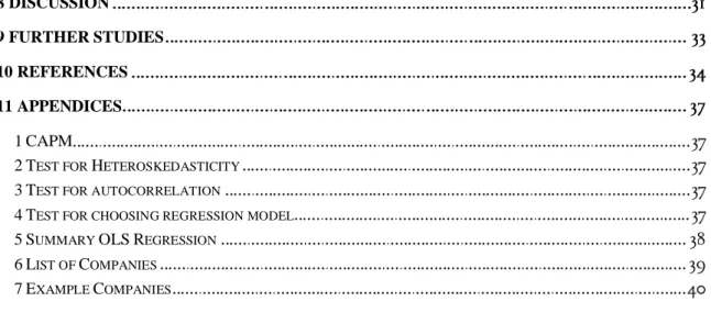
8 DISCUSSION 9 FURTHER STUDIES 10 REFERENCES 11 APPENDICES
1CAPM
2TEST FOR HETEROSKEDASTICITY
3TEST FOR AUTOCORRELATION
4TEST FOR CHOOSING REGRESSION MODEL
5SUMMARY OLSREGRESSION
6LIST OF COMPANIES
7EXAMPLE COMPANIES
TABLE 1 SUMMARY STATISTICS TABLE 2 SUMMARY REGRESSIONS TABLE 3 SIZE EFFECT
TABLE 4 PRICE TO BOOK TABLE 5 JANUARY EFFECT
TABLE 6 TEST FOR HETEROSKEDASTICITY TABLE 7 TEST FOR AUTOCORRELATION TABLE 8 TEST TO CHOOSE MODEL TABLE 9 SUMMARY OLS REGRESSIONS TABLE 10 LIST OF COMPANIES
In this chapter the reader will be informed about the background of the topic followed by a presentation about the problem. The purpose and delimitations for this study will also be presented.
There are numerous ways for investors to calculate the expected returns of an asset within the capital markets. One of the most common theories is the Efficient Market Hypothesis by Fama (1970), which state that the price of an asset is fully reflecting the expected return, based on available information. Essentially, this means that investors are risk-averse and sets a fair price on securities, in order to compensate for the risk attached to the asset. There are a wide variety of pricing models that has been used since the 1960s. William Sharpe (1964) and John Lintner (1965) introduced one of the most famous and common asset pricing models called the Capital Asset Pricing Model (CAPM).
The popularity of CAPM is widely due to its simplicity as being a one factor model. However, the model has raised concerns regarding its ability to set accurate prices for assets. Banz (1981), highlighted concerns with the model when investigating the accuracy of CAPM in a highly cited article. Banz concluded that the model could be misleading. The underlying assumption for this statment is that there was a significant difference in risk-adjusted returns between small and large firms listed on the New York Stock Exchange. Banz also states that the findings have no theoretical explanation at the time, but highlights that this certainly is a topic that need further research.
These findings laid the foundation for further developments of asset pricing models during the following years. As a result, the Fama and French three-factor model was developed and new parameters were added, such as the size premium. (Fama & French, 1992) However, in recent years it has started to become questionable if size should be considered when pricing assets. Recent studies by Ahn and Yoon (2019) have suggested that the size effect was present during Banz interval (1926-1975), but has diminished over time. A study by Asgharian and Hansson (2008) investigated the size effect on the Swedish stock market (OMX) during the time period 1983-1996 and found no evidence that could prove a size effect.
Three years after Banz (1981) study, Keim (1983) presented results that changed the view on the size effect. Keim (1983) referred the presence of the size effect to the existence of a “January effect”. This well-known anomaly was first studied by Watchel (1942) who found a bullish tendency from December to January for the Dow-Jones industrial average during the years 1927-1942. Furthermore, Roseff and Kinney (1976) found results that strengthened Watchels case and concluded that there was a January effect present on the New York Stock Exchange during 1904-1974. Studies by Keim (1983) and, Haug and Hirschey (2006), have found that the January effect could be a small-cap phenomenon, and both of these studies suggest that the presence of the size effect could be referred to the January effect.
When measuring the size of a company, there are different measures to consider. Market Capitalization is basing the size solely on the equity shareholders of a company. Enterprise Value on the other hand, is considering the equity shareholders and the debtholders. Hence, it is considering the full capital structure of a company. Since small-cap companies often are financed by debt, this measure will be used in this paper. (Esperanca, Gama, & Gulamhussen, 2003) To sum up, this study will investigate the size effect when considering the Enterprise Value and the January effect on the OMX during the time period 2000-2019.
Previous research on the size effect is scarce on the Swedish stock market (OMX). However, Asgharian and Hansson (2008) found that the relation between returns and size based on Market Capitalization is insignificant. Hence, there is a possibility that modern asset pricing models, such as the Fama and French (1992) three-factor model, include parameters that lacks significance. As Asgharian and Hansson (2008) and, Ahn and Yoon (2019) suggests, if the size effect has vanished, size is a parameter that perhaps should not be included in an asset pricing model since it has no attribution.
Yet, no studies have been made on OMX when measuring the entire size of a company. As Market Capitalization is only determining the equity value of a company it is not considering the debt. This study will use Enterprise Value as the substitute, in order to include both the equity shareholders and the debtholders of a company. Hence, using Enterprise Value in this study could provide new perspectives on the size effect.
Furthermore, as Keim (1983) and, Haug and Hirschey (2006) suggest that the size effect could be explained by the seasonal anomaly called the “January effect”, this paper will investigate if the January effect is present along with the size effect or if the two market effects have lost their relation.
The first purpose of this paper is to investigate if the size effect is present within the Swedish stock market (OMX) when using Enterprise Value as the factor for size.
Secondly, this paper will examine if the January effect is active on the Swedish stock market (OMX). This study will also investigate if the January effect is a small-cap phenomenon that could possibly explain the size effect.
The scope of this study had to be limited into two main areas where time and geographical matters had to be decided. The first study on the topic was done in 1981, discussing data between 1926-1975. (Banz, 1981) Since then, studies have either accepted or rejected his theory, for example the study by Ahn and Yoon (2019). To make this study relevant and up to date, recent data collected from 2000-2019 will be used in order to get applicable results.
Secondly, the geographic scope had to be considered. This study desires to investigate whether or not the size effect is present in the Swedish stock market (OMX). Earlier studies such as the one by Banz (1981) have had its scope on larger markets, such as the New York Stock Exchange. This study will only be considering stocks listed on the OMX.
This chapter will introduce relevant background information that will be used throughout the study and referred back to. Firstly, the Efficient Market Hypothesis will be introduced followed by two common asset pricing models. Lastly the factors that are included in the modified model for this paper will be presented.
The capital market serves to allocate possession of assets across owners. In the ideal world, the market prices should describe the actual and correct value of an asset. If all information were available to everyone and the investors were being rational, there should not exist any mispriced assets on the market. (Fama, 1970)
When considering an efficient market, one needs to define the conditions of such a market. For a market to be considered as efficient, there are a few criteria that are assumed. (Fama, 1970)
• There are no transaction costs in trading securities.
• All available information is costless available to all market participants.
• All agree on the implications of current information for the current price and distributions of future prices of each security.
There is obviously no such state in reality that fully satisfies all these criteria. This kind of idealized market efficiency will therefore not be available. However, this is a state that is handy to assume when valuing assets.
The Efficient Market Hypothesis has dealt with numerous challenges, such as excess returns and anomalies. Fama (1970) suggests that in an efficient market, the assets should already be accurately priced, hence, excess returns should not exist. The explanation for why excess returns exists in efficient market theory have been referred to as the Random Walk. Fama (1965) means that the “Random Walk” explains that price changes are independent and not predictable or systematic. Furthermore, the ”walks” should be equally distributed across the assets. This phenomenon suggests that it is impossible to predict the path of a stock in an efficient market, all excess returns are random since the asset should constantly be accurately priced.
A recent study by Urquhart and McGroarty, (2016) examined this hypothesis from 1990-2014 on S&P500 (U.S Stock Exchange), FTSE100 (London Stock Exchange), NIKKEI225 (Tokyo Stock Exchange) and EURO STOXX 50 (European Index). This study found that stock returns in some cases can be predictable, but it does vary over time. The authors conclusion was that investors should assess each market independently since each market experience different levels of predictability, based on the market conditions.
The cost of equity is one of the most common and significant factors in capital allocation and corporate valuation. Cost of equity was first introduced by Treynor, Sharpe and Leitner (1964) when the three of them presented the Capital Asset Pricing Model (CAPM). The model came to be one of the keystones in modern portfolio theory and is commonly used within finance.
The assets expected return, which is called the cost of equity in the model, is calculated based on its sensitivity/correlation to fluctuations of the market portfolio (market index). In the CAPM formula, this sensitivity is measured by the value of Beta (β). The complete formula is done by adding the risk-free rate to the firm’s risk premium. The specific firm’s risk premium is calculated by multiplying the Beta with the market risk premium, which is the expected market portfolio return minus the risk-free rate. Hence, Beta is the only “asset-specific” value that is used in this formula. The full formula is presented in appendix 1 CAPM. (Sharpe, 1964)
However, previous studies, such as the one by Banz (1981), suggests that the model does not consider parameters that might be necessary when calculating expected returns, such as size.
Additions to the CAPM has been developed since it was first introduced. Banz (1981) was one of the most influential to present evidence against the model. Banz (1981) found evidence that smaller firms in general provide greater risk-adjusted returns than larger firms, which could not be explained by using the CAPM. This led to extensions of the CAPM being introduced. One of the models that were introduced is called the Fama-French three-factor model which includes size as one of its parameters. (Fama & Fama-French, 1992)
Fama and French presented the three-factor model in 1992, with the purpose to be an extension of the CAPM. In addition to the CAPM, this model considers SMB (Small-minus-big) and HML (High-minus-low) to calculate the expected returns of an asset. SMB estimates the historic excess returns of small-cap companies over large-cap companies, also called the “size effect” (this value is sometimes referred to as the ”size premium”). HML considers the book-to-market value of companies, this value is referred to as the ”value effect” (or value premium). Once both SMB and HML are determined, these variables are added to the CAPM. In the CAPM, Beta (β) is used to calculate 𝑟𝑖 which is the cost of equity (𝐸[𝑟𝑚] − 𝑟𝑓). In the Fama and French three-factor model, Betas (β) are used for the HML and the SMB as well, consisting of the different factors coefficient (sensitivity). The last two parameters include the risk-free rate and the market portfolio returns, denoted by 𝑟𝑓 and 𝑟𝑚.
Below is the complete formula for the Fama and French three-factor model: (Fama & French, 1992)
𝐸[𝑟] = 𝑟𝑓+ β1∗ [𝐸[𝑟𝑚] − 𝑟𝑓] + β2∗ 𝑆𝑀𝐵𝑖+ β3∗ 𝐻𝑀𝐿𝑖
The three-factor model is the first one amongst the Fama and French models, but the duo have thereafter developed additions. In 2015, Fama and French developed a five-factor model. The Fama and French five-factor model also considers the ”profitability factor” and the” investment factor” as additional parameters. (Fama & French, 2015)
The five-factor model:
𝐸[𝑟𝑖] = 𝑟𝑓+ β1∗ [𝐸[𝑟𝑚] − 𝑟𝑓] + β2∗ 𝑆𝑀𝐵𝑖+ β3∗ 𝐻𝑀𝐿𝑖+ β4∗ 𝑅𝑀𝑊𝑖 + β5∗ 𝐶𝑀𝐴𝑖
𝑅𝑀𝑊𝑖= 𝑡ℎ𝑒 𝑟𝑒𝑡𝑢𝑟𝑛 𝑠𝑝𝑟𝑒𝑎𝑑 𝑜𝑓 𝑡ℎ𝑒 𝑚𝑜𝑠𝑡 𝑝𝑟𝑜𝑓𝑖𝑡𝑎𝑏𝑙𝑒 𝑓𝑖𝑟𝑚𝑠 𝑚𝑖𝑛𝑢𝑠 𝑙𝑒𝑎𝑠𝑡 𝑝𝑟𝑜𝑓𝑖𝑡𝑎𝑏𝑙𝑒
𝐶𝑀𝐴𝑖 = 𝑡ℎ𝑒 𝑟𝑒𝑡𝑢𝑟𝑛 𝑠𝑝𝑟𝑒𝑎𝑑 𝑜𝑓 𝑓𝑖𝑟𝑚𝑠 𝑡ℎ𝑎𝑡 𝑖𝑛𝑣𝑒𝑠𝑡 𝑐𝑜𝑛𝑠𝑒𝑟𝑣𝑎𝑡𝑖𝑣𝑒𝑙𝑦 𝑚𝑖𝑛𝑢𝑠 𝑎𝑔𝑔𝑟𝑒𝑠𝑠𝑖𝑣𝑒𝑙𝑦
As explained by Fama and French (2015), the profitability factor (RMW) suggests that companies that has reported higher earnings should obtain higher returns in the long term.
The investment factor suggests that companies that are reinvesting profits in major projects are likely to experience losses in the capital markets, as investors can be investing in the short-term and do not appreciate short-term losses. The profitability factor is collected by checking the operating profit of the company, while the investment factor is obtained by using the year-on-year change in total assets.
The five-factor model has been evaluated by researchers since it was first introduced. Fama and French (2017) tested the five-factor model internationally to find if the factors also were found significant in global markets (Europe and Asia Pacific). However, Fama and French (2017) concluded that the model fails to capture the low average returns of small-cap stocks. This is because the model is considering profitability and investments as factors. Small-cap companies usually spend lots of money on investments rather than profitability in the earlier stages, resulting in a lower valuation according to the five-factor model. (Fama & French, 2017)
Because of the weakness of capturing the valuation of small-cap stocks, this paper will not use the Fama and French five-factor model. For this research, the Fama and French (1992) three-factor model is more suitable.
In corporate finance, firm size is commonly used as a fundamental characteristic. Dang, Li and Yang (2018) found that the coefficient on regressors could show significant difference depending on which measure for size that is applied when observing North American data from CRSP (Center for research in security prices index) during 1993-2006.
Fama and French (1992) measured the size of a company by looking at the Market Capitalization of a company. Market Capitalization is considering the equity value of a company, meaning the value of all shares multiplied by the share price. This is a common approach to get the size of a company entirely based on equity. However, since studies such as Asgharian and Hansson (2008) and, Ahn and Yoon (2019), found no size effect when using Market Capitalization, it would be interesting to investigate the findings when considering another measure for size.
The Enterprise Value of a company equals the Market Capitalization plus debt, minority interest, preferred shares followed by deducting the cash. Hence, the Enterprise Value is considering both the equity shareholders and the debt holders. (Damodaran, 2012)
A study by Esperanca et. al (2003), investigating the capital structures of small-cap companies on the Portuguese market from 1992-1996, found that managers of small-size companies usually issue more debt than equity. This is because managers wish to keep as many shares as possible within the company in the growing phases of the business. Therefore, using Enterprise Value as the measure for size makes sense when investigating a size effect, which is based on small-cap firms performance.
Furthermore, Enterprise Value has been used as the measure for size when investigating a size effect within the Indian stock market during the period 1990-2003. The study by Sehgal and Tripathi (2005) used Enterprise Value among other measures (Net annual sales, Total assets etc.) in order to consider the full capital structure of a company.
However, a disadvantage when using the Enterprise Value is the possible correlation to the Market Capitalization. As the Market Capitalization is included in the Enterprise Value the factors could correlate. Although, as studies such as Murray and Vidhan (2003) suggests, the capital structures differ among companies and firms are rarely funded entirely by equity, when analyzing American firms from 1971-1998. A study by Abbasali and Esfandiar (2012), observing companies on the Tehran Stock Exchange during 2006-2010, proved that successful companies usually issue more debt than equity in order to use leverage to grow the business, suggesting that the correlation does not have to be an issue. Furthermore, as Esperanca et. al (2003) suggests, small-cap companies are usually mainly funded by debt, which results in a less correlation between Market Capitalization and Enterprise Value. Using the full capital structure to measure size, could therefore be appropriate. Also, a study investigating the size effect based on Enterprise Value has not been conducted on the OMX before.
The total return of a company is an appropriate and frequently used method to calculate the performance of an asset. The total return refers to the development of the share price and other components that can drive the returns, such as dividends and capital gains of a company. When measuring the performance of a company, it is important to look at the full performance of the company and not solely based on the development of the stock price. Therefore, it is appropriate to consider the total return of a company as it is calculated by the stock development including re-invested dividends. (Jones, 2002)
The returns will be calculated using simple returns which accounts for the gains or loss during the specific time period. Simple returns do not consider compounding and is calculated before interest expenses and taxes. Since asset pricing models revolves around expected returns and not expected log returns, this way of measuring returns is appropriate. Furthermore, Fama and French (1992) used simple returns in the three-factor model, which further motivates this decision.
Simple return formula: 𝑟𝑡 = 𝑃𝑡
𝑃𝑡−1− 1
- rt : Return for the specific period.
- Pt: Price for the specific period.
The next item included in the Fama and French (1992) three-factor model is the Price-to-Book (P/B) multiple (value effect). This value compares the book value per share and the price per share. The book value of a company is calculated by subtracting the liabilities from the assets of a firm.
In the study by Asgharian and Hansson (2008) it was found that this factor had significant impact on returns, when observing the Swedish stock market (OMX). This factor will be included in the modified model used in this study, in order to compare the significance with the size factor. However, this value will only be used as a benchmark, no further discussion will be conducted based on the results of the “value effect”.
This chapter will introduce the reader to the area of market anomalies in the field of finance. Furthermore, a review of the current available literature is presented.
In 1981, Banz raised concerns for the capital asset pricing model (CAPM) when studying the empirical relationship between the size and returns that the model failed to define. The CAPM, which defines a linear relationship between expected return and the risk associated with the asset, lacked the consideration of other parameters that could have an impact in reality. Banz (1981) study showed that smaller firms on the New York Stock Exchange have on average been able to realize higher risk-adjusted returns than large firms during the period 1936-1977. However, this relation does not show a linear relationship, instead it is fluctuating, which is not what the CAPM suggests.
The findings by Banz (1981), regarding the CAPM, caught the attention for future studies and size were later developed to be one of the parameters in Fama and French three-factor model that was established in 1992. However, even though the size effect has been generally approved since the appearance of the three-factor model, recent studies have raised concerns regarding Banz findings. (Ahn & Yoon, 2019)
In a study by Van Dijk (2011), the author suggests that it is premature to conclude that the size effect as disappeared. Van Dijk’s (2011) study was conducted by reviewing thirty years of research on the size effect (1980-2010), in order to try and explain the phenomenon. Van Dijk (2011) found that the size premium was positive and large in the U.S. even after 1981. Furthermore, the author is suggesting for further research on this area to explain the shifts in the size effect in the past decades. Past theories that have tried to provide explanations for the size effect has neither been systematically tested nor sufficiently developed. Hence, new research could break the deadlock in an area of academic finance literature that has implications for the understanding of asset valuation. (Van Dijk, 2011)
Furthermore, a study by Kato and Schallheim (1985) found a presence of the size effect on the Japanese stock market during the period 1952-1980. The study also found remarkable similarities in terms of the size effect when compared to the U.S. stock markets. Kato and Schallheim (1985) concluded that the similarities between the capital markets could be indicative of well-integrated global markets.
When observing smaller markets internationally, the results differ. A study by Karasneh and Almwalla (2011), investigated the size effect on the Amman Stock Market in Jordan during the time period 1999-2010. This study found evidence suggesting that the size effect is present. Furthermore, the study believes that the size effect could be a phenomenon active specifically in emerging markets. The size effect was also found significant within the Indian stock market between 1990-2003. Sehgal and Tripathi (2005) investigated the size effect based on Enterprise Value, Total Assets, Net Annual Sales etc. and found a significant size effect in all cases. These studies were made on markets that are a lot smaller, compared to the U.S. capital markets and the results are therefore not appropriate to generalize from. By that, it would be interesting to investigate the Swedish stock market (OMX) in order to find if the phenomenon is present within this market.
Research about the size effect within the OMX is very limited. Asgharian and Hansson (2008) analyzed cross-sectional stock market returns for the OMX during the years 1983-1996. The authors were not able to find any evidence of a size effect during that sample period. Asgharian and Hansson (2008) suggested that the size factor was insignificant for the period analyzed. These results are contradicting to what Fama and French (1992) suggested, namely that the size factor should be considered when valuing assets.
Furthermore, a recent study by Ahn and Yoon (2019) analyzed the U.S. stock market between 1950-2012. This study did not find any support for the existence of a size effect. Ahn and Yoon (2019) believes that the lacking empirical support for the size effect after the 1980’s, could be explained by disturbances in the business cycle. When decomposing the business cycle into four distinct stages of drought, expansion, peak and recession, the findings were that the size effect was only significant during the drought period. These findings mean that the size effect is only present during one of the four stages in a business cycle, namely the drought period. Hence, the study suggested that the size effect is a factor that is dependent on macroeconomic structures.
One potential explanation why the effect can be observed during drought periods, could be that small firms can take advantage of the potential rebound on the market and benefit more from improvement in credit market conditions according to Ahn and Yoon (2019). The transition from times with recession to a more expansionary state could have a more rapid impact on sensitive small stocks.
A recent study by Qadana and Aharon (2019), analyzing the U.S. capital market during the time period 1926-2014, discusses other psychological factors, such as the size effect being driven by investors sentiments. Positive sentiment drives the risk aversion down and could potentially increase the size effect as smaller sized companies attract investors who recognize positive sentiments towards the market. These behavioral factors go in line with Ahn and Yoon’s (2019) findings, that the size effect is more present at the turnaround from recession towards expansion. When investors perceive positive sentiments from macroeconomic factors such as an expansion during a business cycle, the size effect could supposedly be increased since risk aversion have a negative correlation with the positive sentiment. (Qadana & Aharon, 2019)
In the field of unexpected market behavior, anomalies have appeared. Anomalies are reached when theory fails to account for the results. When investors are able to predict anomalies, advantage could be gained and abnormal returns realized. The presence of anomalies in the capital markets does not go in line with the Efficient Market Hypothesis and has to be seen as a deviation from the norm. Anomalies that are related to the Efficient Market Hypothesis will not fulfill a nonzero risk-adjusted return (RAR). When stock is providing a fair return corresponding to its specific risk it gives a zero RAR. Stocks that generates positive risk-adjusted returns provides a higher return than what is expected and negative vice versa. When the risk in theory is correct measured the expected RAR should always be zero. (Zacks, 2011)
The anomaly relevant for this study has been introduced in the previous chapters of this paper, namely the January effect. In this section the anomaly will be explained in depth and applicable literature on the topic will be presented.
This anomaly was first studied by Watchel (1942) who found a bullish tendency from December to January for the Dow-Jones industrial average during the years 1927-1942. Rozeff and Kinney (1976) reported a similar seasonal relation in stock market returns, using historical stock prices on the New York Stock Exchange for the period 1904-1974 (with the exception of 1929-1940). The study were able to identify that firms were performing a lot better in January, compared to the other months. The excess returns in January were found to be remarkably higher than the rest of the months and in some cases as much as eight times higher.
Referring to the January effect as an explanation for the size effect was done in 1983. Keim (1983) conducted a study on the New York Stock Exchange, to examine the relation between the size effect and the January effect. The results on the period 1963-1979 suggested that the size effect is heavily driven by the abnormal returns in January, compared to the remaining months. January itself contributed to almost fifty percent of the size effect.
Furthermore, Blum and Stambaugh (1983) found that using closing pricing as reference data points have resulted in a positive bias towards the size effect. When investigating the New York Stock Exchange and the American Stock Exchange during 1963-1980, different results have been reached when applying a buy and hold strategy since the bid-ask spread will not play a role. When conducting such a study, the size effect was downsized to the half. The remaining half, is considered to be the result of small-cap stocks being affected by the January effect. Furthermore, a study by Haug and Hirschey (2006), investigating the American Stock Exchange and the New York Stock Exchange between 1927-2004, suggested that the January effect is largely a small-cap phenomenon and could potentially be the reason for the size effect. The authors found that small-cap firms were affected a lot more than the larger firms. The excess returns for small-cap companies were remarkably consistent even after 1974, which was the endpoint of Rozeff’s (1976) study (1904-1974). A study by Reinganum (1983) suggests that the January effect exists and is stronger for small-cap companies, but Reinganum referred it partly to tax-loss selling. The first trading days of January are providing extraordinal returns for small firms.
Reinganum (1983) found that this is because of the tax-loss selling’s that boost the small firms at the beginning of the year. However, the author also explains that the tax-loss selling’s cannot fully explain the phenomenon, since the rest of January also is strong. But tax-loss selling does have a positive effect to the January effect.
Dahlquist and Sellin (1996) investigated the January effect on the Swedish stock market (OMX) from 1919 to 1994. The study found a strong January effect present on the OMX during this time period. Furthermore, the authors did not suggest that the effect was because of the tax-loss selling which earlier was suggested by Reinganum (1983). The study by Dahlquist and Sellin (1996) could conclude that the January effect was present on the OMX, but it could not explain why. Dahlquist and Selling (1996) did however, not investigate if the effect is stronger for small-cap companies.
Furthermore, there are studies suggesting that the January effect could occur because of a phenomenon called “window dressing”. Lakonishok et. al (1991) studied this phenomenon on the American Stock Exchange and the New York Stock Exchange between 1985-1989 and suggested that large institutional investors will cut embarrassing losses and buy ”safe” winners at the end of the year, ahead of the important reporting period. Though, the concept of large institutional investors investing in low volatility (less risky) stocks would mean that “window dressing” is a large-cap phenomenon, since small-cap stocks usually have higher Beta values. This means that Lakonishok et. al (1991) are suggesting that the January effect is a large-cap phenomenon. Hence, window dressing can explain the January effect, but it does not go in line with the later findings by Haug and Hirschey (2006), who suggested that the January effect is a small-cap phenomenon.
This chapter will give the reader an understanding of how the results of this study has been obtained. It will discuss the data that has been collected and how it has been used to underline different results. Furthermore, this chapter will also highlight the possible shortcomings of the methodology and how these are handled in order to determine results and analysis.
In research there are different types of collectible data that is mainly divided into two categories, quantitative and qualitative. Quantitative data is based on numeric variables which is analyzed through statistics and diagrams. It is concerned with stating facts. Qualitative data on the other hand, are collected through observations, interviews etc. and is used to understand reality. For this study the source of data will be historical stock prices and multiples, which implies the use of quantitative data. The tests will further be done by using statistical measures, hence, a quantitative approach is most suitable. (Saunders, Lewis, & Thornhill, 2016)
The sample of companies for this research has been collected to avoid any selection bias. Banz (1981) included all available companies on the New York Stock Exchange in the research to avoid any selection bias. This method would result in over 300 companies on the OMX and approximately 100.000 observations. Hence, the sample had to be limited in order to interpret and handle the data. This study will use a sample of companies on the OMX that has been active every year from 2000-2019, resulting in 150 companies and approximately 40.000 observations. A list of the included companies can be found in appendix 6.
The data has been collected from NASDAQ OMX Stockholm using a Thomson Reuters terminal supported by Jönköping University. Historical data from year 2000-2019 including closing prices, Price-to-Book ratios and Enterprise Values has been collected on monthly basis. Furthermore, the risk-free rate was collected from the Swedish Riksbank (2020) using the 10-year Swedish government bond. The 10-year bond is commonly used as the measure for the risk-free rate as it is a reasonable investment horizon. The data will be analyzed using the statistical software program STATA, supplied by Jönköping University.
When conducting research there are different ways to perform and execute the studies. Saunders et. al (2016), presents two main approaches, deduction and induction. The process of induction is to collect data and secondly develop theory and hypothesis about the subject. However, for this study the most appropriate way is deduction. In deduction the researchers start with the theory and then develops the hypothesis to be tested. The next step is to collect and test to see adequately if it is true or not through observation.
There are also different purposes with dissimilar kinds of research. This thesis aims to provide answers to relations in the stock market which implies an explanatory purpose. Through statistical tests the authors will try to clarify the relation between different variables. Other intentions of studies can be either descriptive or exploratory, which will not be the commitment of this particular study. (Saunders, Lewis, & Thornhill, 2016) Different approaches to research imply different philosophies in what way to understand the results. When discussing different philosophies in research, it can be narrowed down to five main categories; positivism, critical realism, interpretivism, postmodernism and pragmatism. (Saunders, Lewis, & Thornhill, 2016) This study has adopted the philosophy of positivism which goes in line with the method commonly used in the field of finance. Positivism focus on facts that can be derived from data through measurements and analysis.
When comparing studies similar to this thesis there are two main approaches to consider when planning the statistical model. The choice of which strategy to use is closely linked to the research question. Using a cross-sectional approach could be described as a snapshot in time to see if a phenomenon is present. The other approach is a longitudinal approach. When applying a longitudinal research, the goal is to see relations over time which can be described as a diary perspective. The aspects of both cross-sectional and longitudinal are comprised in Panel data with observations on several companies over different periods of time. (Saunders, Lewis, & Thornhill, 2016)
In statistics there are several different regression methods that can be used for statistical modeling. Ordinary Least Squares (OLS) is a commonly used regression model within the field of finance. It is used to estimate unknown parameters in a linear regression model. However, the dataset for this study are multidimensional, including data of specific companies and a time dimension. When the data is sorted as panel data, one needs to consider which model that is best suited for the study. There are a wide variety of models that could be used for this sample, in order to select the most appropriate one, an F-test and a Breusch and Pagan Lagrangian multiplier test was conducted together with a Hausman test. These tests are evaluating whether to use a Fixed Effects regression, Random Effects regression or an Ordinary Least Squares regression. The results suggested that the Fixed Effects regression would be most appropriate for this study, hence, this regression will be used. The results from these tests are found in appendix 4.
However, when further testing the data sample, issues regarding heteroscedasticity appeared. Therefore, a robust model had to be applied in order to consider the heteroscedasticity. (Angrist & Pischke, 2009)
The Fixed Effects regression is based on panel data in a cross-sectional analysis where a time series dimension is available. The observation will include 𝑛 companies for 𝑡 periods of time. This accounts for unobserved individual heterogeneity by allowing specific interceptions for the individual samples. The slopes of the regression are still common across units, while the intercepts are allowed to vary. Allowing this enables the control for unobserved factors that are time constant. (Woolridge, 2001) In addition to the Fixed Effects Regression, results from the OLS regressions will be available in appendix 5. However, the results from the OLS regressions will not be presented in the result section, instead these regressions are included in the appendix if the reader would like to compare the results between the different regressions.
When conducting sregressions in statistical models, errors are assumed to have the same (but unknown) variance, which implies that disturbances are homoscedastic. It is also assumed that the coefficients are fixed. If the requirements of homoscedasticity are not fulfilled there is a chance that the model loses its efficiency which could lead to analytical errors for the estimates as described by Breuch and Pagan (1979). Breuch and Pagan (1979) wrote about this problem and developed a test for considering this issue.
For the Breuch-Pagan test, the null-hypothesis states that homoscedasticity exists and by rejecting the null-hypothesis the test concludes that heteroscedasticity is present. When testing for heteroscedasticity within the data of this study, it occurred that problem with heteroscedasticity was present since the null hypothesis was rejected (The Breuch-Pagan test is presented in appendix 2). Therefore, the use of regular regressions are not accurate. The solution to this problem is to use a robustness in the models, in order to overcome the issue with heteroscedasticity. This regression considers the heteroscedasticity and is used to accurately adjust the results accordingly. (Verardi & Croux, 2009)
When studying data over time, one important aspect that has to be considered is autocorrelation. It explains how the dataset depends on previous observed data in the same timeseries. To test for autocorrelation a Woolridge test was executed. (Wooldridge, 2010) The Woolridge test concluded that there was no issues with autocorrelation for this sample. Results from the Woolridge test can be found in appendix 3.
In order to test the significance of the used model a student’s T-test will be applied. The test will be conducted by testing the null hypothesis against the alternative hypothesis. The hypothesis will be stated as follows:
𝐻0 = no relation between the dependent and independent variables 𝐻1 = there is a relation between the dependent and independent variables
The test generates a p-value which is considered the chance of falsely reject H0. Therefore,
a low p-value must be generated to be able to find a significance relation between the independent variable and the depend variable. To test for significance in this study a corresponding p-value of .05 will be used and indicated by ** in tables.
Values significant at the .01 level will be indicated by *** and at the .1 level with *. This test is used to find if the size effect is significant. The same procedure is applied to see the presence of the January effect.
To test the hypothesis, a Fixed Effects regression model have been computed using panel data. The variable of high minus low (HML) corresponding to the Price-to-Book ratio was included in the test since it is accounted for in the original Fama and French (1992) three-factor model. The HML variable will however not be as discussed as the SMB variable, but the significance will be compared between the two. The Price to Book multiple has proven significant in recent studies (Asgharian & Hansson, 2008) and it will therefore, be interesting to investigate if this multiple still is significant or not, along with the size effect. To see if the January effect could be related to the size effect, a dummy variable has been included corresponding to the first month of each year.
Monthly returns have been used as the dependent variable and using Enterprise Value and Price to Book ratio as the independent variables. The test will initially be done by including the full dataset of companies. Subsets will then be created by dividing the firms into groups consisting of large sized companies and companies of smaller size.
In order to cluster companies into groups based on Enterprise Value, intervals had to be determined. The general standards by NASDAQ (2013) measures a large-cap company as a company above one billion EURO in Market Capitalization and a small-cap company below 150 million EURO in Market Capitalization. For this study the intervals will be adjusted into SEK and also increased to be appropriate for Enterprise Value.
As NASDAQ (2013) intervals are entirely based on equity value, these intervals have to be adjusted in order to consider the debt of a company. The reviewed articles, such as Abbasali and Esfandiar (2012) and Esperanca et. Al (2003), suggest that companies are usually financed with a debt/equity ratio above fifty percent. Though, to reduce the risk of overexaggerating the intervals, this research will assume an average debt/equity ratio of fifty percent. This means that the intervals for Market Capitalization have been doubled, in order to achieve a capital structure that is financed equally by debt and equity.
Thus, the selected intervals will be 3.25 billion SEK for small-cap and 21.5 billion SEK for large-cap (300 million EURO for small-cap and two billion EURO for large-cap). The consequences of not increasing the intervals would be that the small-cap subgroup would be severely reduced since the Enterprise Value usually is higher than the Market Capitalization.
It would basically mean that a company with 200 million EURO in Enterprise value, financed 70% by debt and 30% by equity would be excluded from the small-cap subgroup even though the Market Capitalization of the company equals 60 million EURO.
However, increasing the intervals also means that a company heavily financed by equity can be considered a small-cap even though the Market Capitalization exceeds 150 million EURO. Yet, the intervals had to be modified and as Abbasali and Esfandiar (2012) and Esperanca et. al (2003) suggests, the debt ratio is usually above fifty percent, these intervals are not considered to be excessive.
The Fixed Effects model is presented down below:
𝐸[𝑟𝑖𝑡] = 𝑟𝑓 + β1∗ 𝐸𝑉𝑖𝑡 + β2∗ 𝐻𝑀𝐿𝑖𝑡+ 𝐷𝑖𝑡+ 𝜀𝑖 𝑖 = 1, … , 𝑛 𝑡 = 1, … , 𝑇
In this model E[rit] equals the monthly returns. The risk-free rate is denoted rf and collected
from Riksbanken (10-year government bond). Beta is denoted by β and represents the specific factors coefficients. The Enterprise Value is denoted EVit and the Price to Book
ratio is represented by HMLit. A dummy variable for the first month of the year is included,
namely Dit, to represent the January effect. Finally, εi is an error term that always should
be considered in models. The same arrangement will be used for the OLS Regression but without indices in a and the time factor t.
A variety of sources have been used to gather information regarding this study. A predominant chice of peer reviewed journal articles has been cited. Among the cited journals there are several well-known such as: Financial Analysts Journal, Journal of Econometrics, Journal of Portfolio Management and Finance, Journal of Banking and Journal of Finance.
Most of the cited articles in the journals used are from the millennium and forward, which is considered to be up to date on this topic. Banz original study on the size effect is from 1981, hence, there is a gap in the literature. The January effect was first found in 1942 by Watchel and later strengthened in 1976 by Rozeff and Kinney.
The older studies on this subject usually identifies the problem itself, while recent studies often try to test for the problem. This study will mainly compare its results with the recent studies to see if the evidence could be strengthened or questioned.
The source of gathered data is available and distributed by a Thomson Reuters terminal supported by Jönköping University. Concerns about reliability and validity is considered by using a long-time horizon of nineteen years of accessible data. The data is tested by generally applicable statistics which does not make it difficult to copy this method for further studies on this area.
The choice of model, which is a modified version of the Fama and French (1992) three-factor model, is designed to be able to capture the relationship between Enterprise Value and return, but also the performance of companies in January. The part that distinguish the model used in this paper from the original Fama and French (1992) three-factor model, is the choice of measure for size, where Enterprise Value have replaced Market Capitalization.
The choice of Enterprise Value instead of Market Capitalization is partly motivated by the fact that Asgharian and Hansson already conducted a study on the size effect for the Swedish stock market (OMX) in 2008, using Market Capitalization. Furthermore, Enterprise Value takes the full capital structure of a company into consideration. Measuring size solely based on equity is not considering the entire size of a company. Enterprise Value has been used to detect a size effect in other international markets, but no previous study has investigated the OMX based on this measure. (Sehgal & Tripathi, 2005)
However, as mentioned in the theoretical background, a disadvantage when using the Enterprise Value could be the possible correlation with Market Capitalization, since the Market Capitalization is included within the Enterprise Value. Although, as studies such as Murray and Vidhan (2003) suggests, the capital structures differ among companies and firms are rarely funded entirely by equity. Studies have proven that efficient companies usually use leverage to grow, rather than equity. (Abbasali & Esfandiar, 2012) Hence, the correlation does not have to be critical. Additionally, as Esperanca et. al (2003) suggests, small-cap companies are typically more funded by debt, which should result in a decreased correlation between Market Capitalization and Enterprise Value.
Another element in this study that could be subject to criticism is the intervals used in this research. The choice of intervals for the subgroups are motivated by the general standards applied by NASDAQ (2013), based on Market Capitalization. The reasoning behind the increase of these boundaries are derived from the fact that Enterprise Value considers the full capital structure and not solely the equity value of a company. The Enterprise Value will therefore usually be higher than the Market Capitalization, since companies are rarely funded exclusively by equity. The specific choice of 3.25 Billion SEK for small-cap and 21.5 Billion SEK for large-cap are motivated by assuming an equally distributed debt/equity ratio, hence doubling the Market Capitalization intervals (150 million EURO to 300 million EURO etc.). However, these intervals are exposed to the risk of assigning companies into the wrong subgroup, which potentially could affect the results.
In this chapter all results from the regressions will be presented for the reader to observe. Furthermore, a summary of the data sample will be included in the summary statistics paragraph.
A summary of the data sample with all subgroups can be found in below. Findings to highlight are the distinct difference in standard deviation across the three sets for returns. As can be seen in the table of summary statistics, the full sample provided a standard deviation of returns corresponding to 0.148. Though, when analyzing the two subsets of small-cap firms and large-cap firms, it shows that the smaller subgroup has a standard deviation of 0.177 while the large-cap subgroup has a standard deviation corresponding to 0.088. This shows that the group including small-cap has considerably higher standard deviation than the subgroup including large-cap companies. Hence, these results suggest that small-cap firms are exposed to higher fluctuations in their returns compared to large-cap firms.
Further comparisons between the subgroups states that the mean returns appear to be lower for small-cap firms, with a mean value equal to 0.84% compared to 1.35% for large-cap and 1.13% for the full sample. Suggesting that small-cap firms provide less returns than large-cap firms.
The sample size consists of approximately 40.000 observations in the full set. Within the full sample, roughly 19.600 observations corresponds to the small-cap companies and 11.500 to the large-cap. The remaining observations are allocated within the companies in between the intervals for the subgroups.
Variable Obs Mean Std. Dev. Min Max
Full sample
Return 39830 0.0113 0.14866 -1 8.31677
Enterprise value 38694 57.441 181.316 -0.6412 1520.72
Price Book value 40059 2.3667 58485.8 -86.81 1.17E+07
EV > 21,5
Return 11525 0.0135 0.0882 -1 5.61629
Enterprise value 11564 188.11 294.567 21.6 1520.72
Price Book value 11558 2.4345 9.369 -86.81 1.1E+07
EV < 3,25
Return 19613 0.0084 0.17749 -1 8.31677
Enterprise value 19908 0.7724 0.80210 -0.64128 3.2476
Evaluation for the dataset had to be done by conducting two additional tests to investigate if the results could be misleading because of issues with heteroscedasticity and/or autocorrelation. A Breusch-Pagan test were executed which showed that the data had problems with heteroscedasticity. To adjust for this issue robust regressions were conducted for further tests. To test for autocorrelation a Wooldridge test was conducted and the result showed no implications with autocorrelation. Results from the Breusch-Pagan test and the Wooldridge test are displayed in appendix 2 Test for Heteroskedasticity , and appendix 3 Test for autocorrelation.
The results from the Fixed Effects regressions are presented in below.
This table gives an overview of the significance levels and coefficients of all factors for the sample. The level of significance is indicated by *, ** and *** with the corresponding levels of .1, .05, and .01. The results will be presented in detail for each factor in the following paragraphs.
Return Coef,
Robust
Std, Err, t P>|t| [95% Conf, Interval] Full
Sample
ENTERPRISEVALUE 2.09E-05 1.47E-05 1.42 0.156 -7.97E-06 4.97E-05
PRICETOBOOK 0.000180*** 0.000048 3.75 0.000*** -0.000086 0.000275
January 0.042684*** 0.002640 16.16 0.000*** 0.037508 0.047860
_cons 0.005876*** 0.001150 5.11 0.000*** 0.003621 0.008131
EV > 21,5
ENTERPRISEVALUE 1.52E-05 9.15E-06 1.66 0.167 -2.75E-06 3.31E-05
PRICETOBOOK 0.000090** 0.000089 1.02 0.031** -0.000084 0.000266
January -0.0017165 0.002959 -0.58 0.562 -0.007517 0.004083
_cons 0.010686*** 0.001901 5.62 0.000*** 0.006958 0.014414
EV < 3,25
ENTERPRISEVALUE 0.015443*** 2.40E-03 6.44 0.00*** 1.07E-02 2.01E-02
PRICETOBOOK 0.000156** 0.000063 2.48 0.013** 0.000032 0.000280
January 0.081103*** 0.004543 17.85 0.000*** 0.072198 0.090008
In the first test for the full sample, all firms ranging from small-cap to large-cap were included to see if there was any relation between the Enterprise Value and returns. This test produced a p-value of .156, which results in a failure of rejecting the null hypothesis since the p-value is not small enough to reject H0 at the .05 significance level. This means
that no relation between Enterprise Value and returns were found on the full sample. Suggesting that there is no size effect found on the full sample. The results from the regressions based on size are presented in down below in .
EV - Return Coef.
Robust Std.
Err. t P>|t| [95% Conf. Interval]
Full Sample 0.0000209 0.0000147 1.42 0.156 -0.00000797 0.0000497
EV > 21.5 0.0000152 0.00000915 1.66 0.167 -0.00000275 0.0000331
EV < 3.25 0.0154433*** 0.0023992 6.44 0.00*** 0.0107407 0.0201459
Furthermore, this study wanted to investigate if there was any relation present within the different subgroups. This was done in order to see if there could be a size effect amongst the smallest companies within the small-cap subgroup. The large-cap subgroup was also included to see if there could be a relation between returns and size even for large companies. For the small-cap subgroup, this test was found to be significant at the .01 level, with a p-value approximately equal to zero. Hence, there is a positive relation between Enterprise Value and returns within the small-cap subgroup.
For the subgroup containing the large firms there was no relation to be found between returns and Enterprise Value. The test resulted in a p-value equal to .167 which is higher than the applied significance level of .05, stating no relation was found. These results mean that a relation between size and returns could only be found within the subgroup of smaller companies.
The Price-to-Book results are included to compare the significance of this factor and the size factor in the Fama and French (1992) three-factor model. The results on the Price-to-Book multiple is presented below in . Significance was found in the full sample and the two subgroups. The highest significance was found in the full sample, a p-value almost equal to zero shows significance at the .01 level which indicates a high significance. The subgroup including the large firms provided a p-value of .031 which is significant at the .05 level. For the group of small companies, the p-value of .013 shows significance at the .05 level. Hence, the test shows that the Price-to-Book multiple is significant for all samples.
P/B - Return Coef. Robust Std. Err. t P>|t| [95% Conf. Interval]
Full Sample 0.0001808*** 0.0000482 3.75 0.000*** -8.6E-05 0.000275
EV > 21,5 0.0000909** 0.0000895 1.02 0.031** -8.5E-05 0.000266
EV < 3,25 0.0001564** 0.0000632 2.48 0.013** 3.26E-05 0.00028
As explained in the literature review, studies have suggested that the January effect is a possible explanation for the size effect. (Keim, 1983) In order to investigate if there was a relation between the size effect and January effect, a dummy variable was included in the test for the first month of each year. Results from the test on the January Effect are presented in below. The tests were first done by including the full sample and subsequently on the two subgroups based on size.
The first test showed strong statistical significance with a p-value close to zero and a coefficient equal to approximately 0.043. Stating that on average, the companies in the full sample was able to provide higher returns for the first month of the year compared to the other months.
January -
Return Coef. Robust Std. Err. t P>|t| [95% Conf. Interval]
Full Sample 0.042684*** 0.0026409 16.16 0.000*** 0.037508 0.047861
EV > 21,5 -0.0017166 0.0029592 -0.58 0.562 -0.00752 0.004084
To examine if the size effect could be explained by the January effect, the same regressions were conducted on the different subgroups based on Enterprise Value.
For the group including large-cap companies a p-value of .562 was found, which exceeds the significance level of .05. Hence, no significant evidence of a January effect were to be found within the large-cap subgroup.
The results from the test consisting of small-cap firms gave a p-value of approximately zero, which implies a strong presence of the January effect at a significance level of .01. Furthermore, the coefficient was almost twice as high for small-cap firms (0.081) compared to the full sample (0.043).
This chapter will analyze the findings from the results and explain what the results suggest. Furthermore, it will compare the results from this study with results from previous studies on the topic.
The results obtained when studying the size effect goes in line with previous studies, such as Ahn and Yoon (2019) together with Asgharian and Hansson (2008). This study did not find any evidence that small-cap firms outperform large-cap firms during the time period 2000-2019 on the Swedish stock market (OMX).
This paper used different data and changed the measure for size to investigate the size effect. Asgharian and Hansson (2008) used data from 1983-1996 in comparison to this study, which uses recent data from 2000-2019. Also, most previous studies have used Market Capitalization as the measure for size, while this research is using Enterprise Value instead. However, the size effect could not be found when using this modified measure for size.
Although, a result that has not yet been presented in previous studies are that there is a reversed size effect within small-cap companies on the OMX, when using Enterprise Value as the measure for size. When doing regressions on the specific subgroups, a positive relation between Enterprise Value and returns within the small-cap firms was found. This means that as small-cap companies increase in Enterprise Value, their returns increase as well, which is contradicting to the original size effect. (Banz, 1981) This result is essentially suggesting a reversed size effect, as the returns increases as the size of a company increases. Furthermore, this means that the lower percentile within small-cap companies, realize less returns than the larger small-cap companies.
In addition to the size effect, this research is considering the January effect and investigating if it is a small-cap phenomenon that could have possibly impacted the existence of the size effect. The results on the full sample quantified that the companies were able to provide larger returns in January compared to the rest of the year, during the time period 2000-2019 on the Swedish stock market (OMX).
The results go in line with previous research on the OMX, such as Dahlquist and Sellin (1996), who suggested that the January effect is active on the Swedish market. However, that study did not consider if the phenomenon was stronger within small-cap companies. In order to find if the January effect is a small-cap phenomenon, tests were conducted on the different subgroups. As the coefficient was found twice as high for the small-cap firms compared to the full sample, this study does support Haug and Hirscheys (2006) claim that the January effect could be a small-cap phenomenon. This is also supported by the fact that the large-cap subgroup showed no significance of realizing greater returns in January compared to the rest of the year.
The findings of this study, goes in line with the research by Asgharian and Hansson (2008), suggesting that there is no size effect present on the Swedish stock market (OMX). Hence, it is hard to motivate why size should have the weight it has in the Fama and French (1992) three-factor model when valuing assets on the OMX.
Previous studies have primarily used Market Capitalization to try and find a significant relation to returns and failed. (Asgharian & Hansson, 2008) This study used Enterprise Value to investigate the impact of the full capital structure on returns. The results showed no evidence that can prove that small-cap firms outperform large-cap on the OMX during the time period 2000-2019.
Hence, the results suggest that size has no impact on the expected returns and one could argue that this parameter should be reconsidered in asset pricing models. The Price-to-Book multiple was tested in order to compare the significance with the size factor. The Price-to-Book multiple showed significance throughout the sample, which was the same results as the study by Asgharian and Hansson (2008), suggesting that this factor still is relevant on the OMX. Perhaps, the size effect was present during the time when Fama and French developed the three-factor model (1992).
However, times are changing, and investors need to adapt to the current market climate in order to achieve success. Using models which include parameters that might not be relevant could be destructive. Hence, investors should adapt to each market independently. For the OMX, this could mean that the size factor should be excluded from the asset pricing models.
This chapter will conclude and highlight the most relevant and interesting findings of this paper.
This research could not detect a size effect on the Swedish stock market (OMX) when observing companies from 2000-2019, when using Enterprise Value as the measure for size. However, a reversed size effect was detected within the small-cap subgroup. The reversed size effect suggests that the lower percentile of small-cap companies realizes less returns than the higher percentile. This could be contradicting to the size effect, which suggests that smaller companies generate higher returns.
Regarding the tests for the January effect, the results showed that the effect is present within the full sample. However, the large-cap subgroup was not affected by the January effect, but within the small-cap subgroup, the coefficient was twice as high compared to the full sample. Hence, this study suggests that the January effect could be a small-cap phenomenon. These results suggest that the January effect has a positive effect on the size effect and could possibly be one reason for the size effect’s presence in history. However, the two market phenomenon’s are not highly correlated anymore, since the January effect is present and the size effect remains absent on OMX, according to this study.
When considering size as a factor in asset pricing models, a convincing and assuring opinion about its influence has been hard to agree upon in earlier studies. Previous research on OMX using Market Capitalization as the measure for size, has resulted in no evidence that the attribution of size should be considered. (Asgharian & Hansson, 2008) This paper decided to use Enterprise Value as the measure for size in order to consider the entire firm size (debtholders and equity shareholders) of companies and could not detect a size effect on OMX.
Hence, this study suggests that size possibly should get less emphasis when valuing assets on OMX. Instead focus should be weighted on reliable factors that has proven significance consistently, such as the Price-to-Book ratio which was found significant in the study by Asgharian and Hansson (2008) and in this paper.
This chapter will discuss the findings of the paper compared to previous studies. Furthermore, this chapter will discuss the methodology and how results could have differed depending on the method for this study.
The purpose of our study was to investigate if the size effect and/or the January effect is present on the Swedish stock market (OMX) when using Enterprise Value as the measure for size. Furthermore, our paper wanted to investigate if the January effect is a small-cap phenomenon that could be an explanation to the size effect.
Our results did not differ from the findings by Asgharian and Hansson (2008), even when substituting the measure for size and the data sample. Though, our research does in fact contribute to the subject. No previous study has tested the size effect when considering Enterprise Value as the measure for size on the OMX. Following that reasoning, no previous study has detected a reversed size effect when using Enterprise Value as the measure for size. Perhaps using this measure could be further examined in asset pricing models, as it is taking the full firm size of companies into account. Using leverage to grow is common amongst small-cap companies and hence, it should perhaps be considered to a higher degree when measuring size. (Esperanca, Gama, & Gulamhussen, 2003)
Furthermore, when considering the January effect, our study complements the study by Dahlquist and Sellin (1996), as their study did not investigate if the January effect was a small-cap phenomenon. Our results contribute to Haug and Hirschey’s (2006) claim that the January effect could be a small-cap phenomenon, when observing the OMX. Therefore, the January effect could potentially have been the reason for the size effect’s prior existence. Today however, the January effect is not able to explain the presence of the size effect. Perhaps the correlation between the market effects was stronger before our time period (2000-2019), nevertheless, the correlation has in fact diminished within the OMX, since only the January effect has been detected in our research.
However, the results of our study are affected by our own assumptions about the capital structures of the companies in our sample. Converting the intervals of small-cap/large-cap companies from Market Capitalization to Enterprise Value is a factor that might have affected our results.