Annelie Carlson
Robert Karlsson
Olle Eriksson
Energy use due to traffi c and
pavement maintenance
The cost effectiveness of reducing rolling resistance
VTI notat 9A-2016
|
Energy use due to tr
af fi c and pav ement maintenance. T he cost ef fectiv eness of r educing r www.vti.se/en/publications
VTI notat 9A-2016
Published 2016
VTI notat 9A-2016
Energy use due to traffic and pavement
maintenance
The cost effectiveness of reducing rolling resistance
Annelie Carlson
Robert Karlsson
Olle Eriksson
Diarienummer: 2012/0354-292 Omslagsbilder: Thinkstock Photos Tryck: LiU-Tryck, Linköping 2016
Preface
The project has been financed by the Swedish Transport Administration and their research programme BVFF. Åsa Lindgren has been the contact person. This work is a part of sub project 3 in the European collaboration MIRIAM (Models for rolling resistance in Road Infrastructure Asset Management Systems). The results from this sub project have been presented at a seminar in Stockholm in May 2015, arranged by the Swedish Transport Administration within the MIRIAM collaboration. It has also been presented at the national conference Transportforum in Linköping January 2016. This documentation is the final report of the project Energy use due to traffic and pavement maintenance – The cost effectiveness of reducing rolling resistance.
Linköping, March 2016
Annelie Carlson Project leader
Quality review
Internal peer review was performed on 28 February 2016 by Iman Mirzadeh. Annelie Carlson has made alterations to the final manuscript of the report. The research director Mikael Johannesson examined and approved the report for publication on 30 March 2016. The conclusions and
recommendations expressed are the author’s/authors’ and do not necessarily reflect VTI’s opinion as an authority.
Kvalitetsgranskning
Intern peer review har genomförts 28 februari 2016 av Iman Mirzadeh. Annelie Carlson har genomfört justeringar av slutligt rapportmanus. Forskningschef Mikael Johannesson har därefter granskat och godkänt publikationen för publicering 20 mars 2016. De slutsatser och rekommendationer som uttrycks är författarens/författarnas egna och speglar inte nödvändigtvis myndigheten VTI:s uppfattning.
Table of contents
Summary ... 7
Sammanfattning ... 9
1. Introduction ... 11
1.1. Background ... 11
1.2. Scope, purpose and objectives ... 12
1.3. Disposition ... 12
2. Description of work ... 13
2.1. Problem formulation ... 13
2.2. Method for the decision procedure ... 15
2.2.1. Criteria for cost efficient maintenance that reduces energy ... 15
2.2.2. Uncertainty and variability and their importance in pavement management... 16
2.2.3. Development of decision making procedure ... 17
2.2.4. Uncertainty in the decision ... 18
2.2.5. Design of case studies ... 20
2.3. Climate ... 30
2.4. VETO ... 31
3. Statistical analysis ... 33
4. Climate ... 36
4.1. Dry road conditions ... 36
4.2. Water ... 39 4.3. Snow ... 41 5. Discussion ... 44 5.1. Valuation of CO2 ... 44 5.2. Decision support ... 45 5.3. Climate ... 46
6. Conclusions and recommendations and support for road managers ... 48
References ... 51
Appendix 1. Simulation results ... 53
Appendix 2. Relative fuel use due to water on the road surface ... 61
Summary
Energy use due to traffic and pavement maintenance – The cost effectiveness of reducing rolling resistance
by Annelie Carlson (VTI), Robert Karlsson (Swedish Transport Administration) and Olle Eriksson (VTI)
Measures in order to reduce GHG exist across a range of policy areas. The transport sector is one of the areas where the potential for a reduction is considered to be of great importance. A large effort has been placed upon making vehicles more fuel efficient and there are regulations within the European Union setting emission standards for new vehicles. However, the impact of the management activities is also an area where there is a potential to reducing energy use of traffic and thereby GHG since almost all fuel used is based on fossil fuel. The reduction can be achieved by performing maintenance measures that lower the rolling resistance, and with the aim of decreasing the total energy use in a life cycle perspective, including energy for both traffic and maintenance.
When choosing maintenance alternative, it is also of importance to consider the costs involved. Pavement management is focused on keeping wide spread road networks in acceptable condition given certain budget constraints. Therefore, the economic constraints need to be addressed and in the case of choosing a maintenance alternative that reduces total energy, it also has to be cost-efficient in order for it to be performed.
The main scope of the research presented in this report is to investigate how road management should act to reduce total energy use of roads, including traffic and maintenance induced energy use, while also taking cost efficiency and the aspect of uncertainty into consideration. The purpose is to enable a better consideration of the total energy used and maintenance cost when managing the road network. The objective is to derive a meaningful instrument for decision making situations such as when selecting and designing maintenance treatments, in which total energy use and maintenance cost is considered.
A general method is developed and presented. A criterion, CR, has been identified for how to choose a pavement maintenance strategy in regards to cost and energy efficiency. A cost benefit analysis approach using Benefit to Cost Ratio, BCR, has been adopted. It is shown that the selection between alternatives is straightforward under certain circumstances and if CR is significantly lower or higher than 0. If CR is close to 0 the variability and uncertainty will be significant and should be taken into account when selecting maintenance alternative.
The study indicates that it is difficult to establish a simple rule of thumb. However, the CR-value may be a useful criterion in some circumstances and it is important to have guidelines as decision support where assessments are made of the road surface characteristics, total energy use and maintenance cost and where the different aspects are valued. This is especially important on an object level.
The effect of traffic energy use due to snow and water on the road surface was estimated. The possibility for taking these aspects into consideration when deciding on a strategy for an energy- and cost effective pavement maintenance is limited. In summary, snow should not be accounted for, but the presence of water on the road surface could be a variable to consider. Moist has a non-negligible effect on fuel use and it is also to some extent dependent on the road surface conditions. However, how this should be done is not considered in the report but it could be interesting to investigate further. It should be emphasized that decision on which maintenance alternative to choose must, in the long run, be based on a broader perspective than just energy and maintenance cost and should also include other aspects of sustainability and safety.
Sammanfattning
Energibehov för trafik och för underhållsåtgärder av vägbeläggning – Kostnadseffektiviteten av att reducera rullmotståndet
av Annelie Carlson (VTI), Robert Karlsson (Trafikverket) och Olle Eriksson (VTI)
Åtgärder för att minska utsläppen av växthusgaser finns inom en rad olika policyområden.
Transportsektorn är ett av dessa områden där man anser att det finns stora möjligheter att få till stånd en reduktion då merparten av bränsle som idag används baseras på fossila bränslen. Ett stort arbete har hittills också lagts på att få mer bränsleeffektiva fordon. Det finns dock även en potential att via vägunderhållsåtgärder, som sänker rullmotståndet, kunna minska energianvändningen hos trafiken. Det är i sammanhanget dock viktigt att se till livscykelperspektiv och även inkludera den energi som behövs till underhållet och att det totala energibehovet minskar. När ett underhållsalternativ väljs, är det också viktigt att ta hänsyn till kostnaderna i och med att det finns budgetrestriktioner. Därför behöver åtgärderna också vara ekonomiskt försvarbara.
I denna rapport undersöks hur man kan välja ett vägunderhåll som minskar den totala energi-användningen för trafik och underhåll, samtidigt som det tas hänsyn till kostnadseffektivitet och osäkerheter. Syftet är att göra det möjligt för väghållaren att bättre ta i beaktande såväl energi som kostnader när de hanterar vägnätet. Målet är att härleda en meningsfull tumregel som kan användas för beslutsfattande när man väljer vilket vägunderhåll som ska utföras där både energi och kostnader ingår.
En generell metod för beslutsstöd har tagits fram och presenteras i rapporten. Ett kriterium, kallat CR, har identifierats vilket kan användas för att bestämma den strategi man ska utgå ifrån när man väljer mellan två underhållsåtgärder. Tillvägagångssättet bygger på en kostnads-nyttoanalys och med hjälp av denna metod har det visats att valet mellan två alternativ är relativt okomplicerat under vissa omständigheter och om CR är betydligt lägre eller högre än 0. Om CR är nära 0 kommer osäkerheter i indata att bli betydande och detta bör beaktas vid val av underhållsalternativ.
Studien visar vidare att det är svårt att fastställa en enkel tumregel. Emellertid kan CR-värdet vara ett användbart kriterium i vissa fall. I rapporten identifieras att det är viktigt att det finns riktlinjer som beslutstöd där man gör bedömningar av energi, kostnader och vägytans egenskaper. Speciellt är detta viktigt på objektnivå.
Effekten av trafikens energianvändning på grund av snö och vatten på vägytan uppskattades också i rapporten. Möjligheten för att ta dessa aspekter i beaktande vid val av strategi för ett energi- och kostnadseffektivt vägunderhåll är begränsad. Kort sammanfattat bör snö inte inkluderas som variabel, medan närvaron av vatten på vägytan kan vara en aspekt att överväga. Vatten har en icke försumbar effekt på bränsleförbrukningen och det är också i viss mån beroende av vägytan. Hur detta kan göras har inte närmare berörts i rapporten men det kan vara intressant att undersöka vidare.
Det bör understrykas att beslut om underhållsalternativ i förlängningen även ska baseras på ett bredare perspektiv än bara energi och underhållskostnader. De bör också omfatta andra aspekter av miljö, hållbarhet och säkerhet.
1.
Introduction
1.1. Background
The focus on climate changes has led to attention on actions to reduce greenhouse gas (GHG)
emissions from road transport in order to mitigate global warming. Emissions from fossil fuels are an important contributor to GHG emissions and efforts are spent on promoting development of
alternative fuels and more fuel efficient engines (European parliament 2009a, European parliament 2009b). Also road management activities themselves contribute to energy use and emissions, but they are in general small compared to traffic fuel use (Karlsson et al. 2012, Carlson 2011, Wang et al. 2012). However, there are reasons to believe that road management can influence the total amount of emissions from road transport by actions influencing rolling resistance. The effect of reducing rolling resistance has for example been shown by Hammarström et al. (2012) where they estimated that a reduction of MPD with 0.5 mm per road link would lead to a decrease in traffic fuel consumption with 1.1% for the road network. Also in Carlson et al. (2013) the effect on energy need due to roughness (IRI) and macrotexture (MPD) was estimated and the evaluation showed that it is possible to lower the traffic fuel consumption by improving IRI and MPD. In Karlsson et al. (2012) the approach of a life cycle perspective on energy use and the importance of rolling resistance was evaluated. The study was performed as a case study of two separate road section with different characteristics and with different maintenance options. It was shown that the total energy use (maintenance and traffic) can be lower by choosing a maintenance alternative that leads to a lower rolling resistance. Also, Wang et al. (2012) used a life cycle approach to analyse the impact of reducing rolling resistance. They concluded that the GHG and energy savings with a reduced rolling resistance can be significantly larger than the energy use and GHG emissions from material production and construction. The savings could also be larger than those from other strategies to reduce traffic energy use, like projected improvements in vehicle fuel efficiency.
The important issue of addressing climate goals is yet to be supported by the current decision making tools and systems. Pavement management today is focused on keeping wide spread road networks in acceptable condition given certain budget constraints. Additional budgets are often released to improve the status of the road network, for example safety and bearing capacity. Therefore, the economic constraints require clear motives in order to choose an alternative taking total energy reduction into account. Pavement management can never achieve one hundred percent optimized decisions with all aspects accounted for. Fair levels of acceptance need to be stated which account for road manager economy (budget constraint), life cycle economy, societal costs, environmental impact, ride quality, traffic safety, health etc. Road manager budget constraints are in practice more rigid than the other aspects, which is one of the reasons for sub optimization, as focus on budgets draws attention from other aspects. Lack of knowledge is another reason. The combination of lack of knowledge and rigid budget constraints may have, as a consequence, that focus shift even more away from aspects difficult to handle to more distinct budget goals and short term quality of pavement performance. Decision makers need to trust the facts presented to them to broaden their focus to a more holistic approach.
This report is a continuation of the international co-operation project MIRIAM (Models for rolling resistance in Road Infrastructure Asset Management Systems). The overall objective of the MIRIAM project is to “provide a sustainable and more environmentally friendly road infrastructure by
developing an integrated methodology for improved control of road transport CO2-emissions”. The
Swedish part, initiated and financed by the Swedish Transport Administration, consists of three sub-projects:
A. Characteristics of the road surface
- A1 Influence on speed due to road surface characteristics - A2 Model to estimate MPD and IRI across the road
B. The effect on rolling resistance due to wet road surface conditions.
C. Total material and energy use with respect to rolling resistance and pavement maintenance in a life cycle perspective.
This report covers the results in sub-project C and specifically addresses the topic of the role of rolling resistance on total energy use and if maintenance treatments can be viable option to increase energy efficiency in a life cycle perspective. The work starts from previous outcome of the same sub project in MIRIAM (Karlsson et al. 2012). A general method/model is developed and presented that can make it possible to take the cost effectiveness into consideration when evaluating the pavement maintenance measures to reduce total energy use. The method should enable the user to decide whether one should choose maintenance measure according to cost or total energy use and the findings of more general relationships can be used for decision making planning and design of pavement maintenance. Also, the effect on fuel use due to precipitation is estimated.
1.2. Scope, purpose and objectives
The scope is to investigate how road management should act to reduce total energy use of roads, including traffic and maintenance induced energy use. The report focus on how road management can reduce traffic energy by lowering rolling resistance of pavement surfaces by decreased macro texture and increased evenness. The cost efficiency of reducing the total energy use is also assessed including the aspect of uncertainty. The issue of precipitation on the surface that increases rolling resistance is as well included in the report.
The purpose of this work is to enable road management to better consider the total energy used and maintenance cost on roads when managing the road network.
The objective is to derive a meaningful instrument for decision making situations such as when selecting and designing maintenance treatments, in which total energy use and maintenance cost is considered. A criterion will be formed for choosing a pavement maintenance strategy in regards to cost and energy efficiency. The objective is also to show the importance of water and snow on traffic energy use.
1.3. Disposition
The work is described in Chapter 2 and the results for the statistical analysis and for the climate aspect are presented in Chapter 3 and in Chapter 4 respectively. The discussion is presented in Chapter 5 and in Chapter 6 comprises conclusions, recommendations and support for road managers.
2.
Description of work
2.1. Problem formulation
Pavement maintenance can reduce rolling resistance by influencing the road surface properties such as macro texture and evenness. Maintenance activities can also change pavement conditions with respect to drainage conditions (cross fall, rut depth, pavement permeability). Road managers will also have to consider other aspects such as road design, speed limits, traffic safety measures, traffic flow capacity etc.
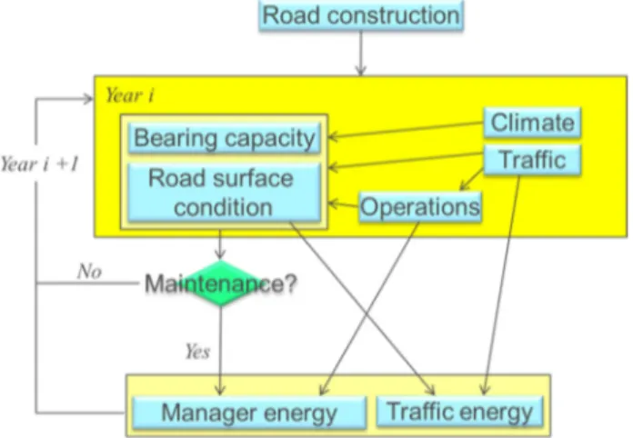
Energy is used by road users and in activities initiated by road managers. The energy used by road users is dependent on the evenness and texture achieved by road management, which means that the decisions made by road management will influence the amount of energy used by road users during a long period. Therefore, calculations need to reflect the change in condition during several years, including the period when road user energy is affected by pavement management decisions. As pictured below this requires a simulation on a yearly basis to accurately reflect how road condition influence road user energy.
Figure 1. Calculation of energy use in incremental steps.
In Karlsson et al. (2012) two case studies were undertaken in which the energy use for traffic and pavement manager induced actions were investigated using a life cycle inventory approach. The calculations were performed by inventory of all activities down to material flow levels or to aggregated levels if no data is available and the calculation of energies was based on a number of sources. The analysis period was based on the period maintenance measures can contribute to performance. If multiple measures are performed, or if the benefits of a measure will be significant beyond the next maintenance measure, a sufficiently long analysis period was chosen to include the complete benefit.
Some of the general conclusions of the study were:
Lower rolling resistance saves fuel for each vehicle passing and by lowering the rolling resistance on highly trafficked roads more energy will be saved.
The larger the influence of rolling resistance is on total fuel consumption, the larger is the influence of a change in rolling resistance. I relation to this, heavy vehicles have more to gain from lower rolling resistance than cars.
Rolling resistance is relatively more important at lower speed compared to higher speed due to the increased importance of wind forces with higher speed.
It is more important to have a low rolling resistance where the vehicles are speeding up or maintaining a constant speed.
It was also shown that it is possible to lower the total energy use for a road section by choosing a maintenance alternative that reduces rolling resistance. In some cases, it can be worth to spend more energy on the maintenance stage if it will lead to lower traffic energy use. However, it may not be feasible to perform maintenance at a higher cost even though the total energy use would be minimised. With a prevailing budget constraint, it is important that the road management is also cost efficient. In order to evaluate the cost effectiveness of reducing the total energy use one can relate the direct cost of reaching the reduction with the social value of the avoided emissions. The direct cost of fuel and a value of the social cost for emission of CO2 according to ASEK 5 (Trafikverket 2015) was applied in a
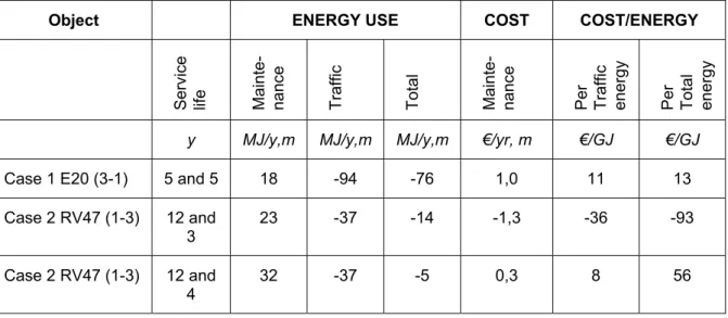
straightforward way to the case studies in Karlsson et al. (2012). The results are shown in Table 1. The difference between the total energy used in different maintenance options range from zero (do nothing) to 525 MJ/m (secondary) and the corresponding cost of 56 €/m for Scenario 2, Case 1. A more relevant comparison is to divide energy and cost by service life. The difference between
Scenario 1 (preferred) and Scenario 3 (least total energy) is an extra 18 MJ/m per year for maintenance and to an extra cost of €1/m per year. The resulting gain in secondary traffic energy is 94 (169 – 75) MJ/m per year. This means an annual saving of 76 MJ/m per year at a cost of €1/m per year, which corresponds to a cost of 13 €/GJ to save energy for case 1 (170 €/ton CO2,assuming 0.075 ton
CO2/GJ). For Case 2 Option 1 and 3 can be assessed as the most realistic ones and therefore they are
compared. It turns out that Option 1 is both the most cost and energy efficient alternative per year, per meter. However, the difference in cost between the alternatives are very small and a simple sensitivity analysis shows that if the service life of Option 3 would increase from three to four years, the
corresponding cost for keeping the more energy efficient Option 1 would be 56 €/GJ.
Table 1. Differences in cost and energy use between alternatives in case 1 and case 2. A sensitivity analysis is included in Case 2 to illustrate effects of small cost difference between alternatives.
Object ENERGY USE COST COST/ENERGY
Serv
ic
e
life Mainte- nan
ce
Traffic Total Mainte- nan
ce
Per Traffic energy Per Total energy
y MJ/y,m MJ/y,m MJ/y,m €/yr, m €/GJ €/GJ
Case 1 E20 (3-1) 5 and 5 18 -94 -76 1,0 11 13 Case 2 RV47 (1-3) 12 and
3 23 -37 -14 -1,3 -36 -93 Case 2 RV47 (1-3) 12 and
4 32 -37 -5 0,3 8 56
With this example it can be concluded that the gain from less fuel consumption can exceed the extra cost of maintenance. But the results turn out to be sensitive to uncertainties and by assuming a service life of one more year for one of the cases meant there is a problem when assessing energy savings in relation to cost in that very small differences in cost will inevitably lead to low cost per gained energy
ratios. In general, predicting future maintenance cost with this accuracy is not possible. The present models available for traffic and maintenance energy use are able to deliver estimates for traffic energy based on ideal conditions and for maintenance energy based on assumptions on the practice used in material production, service life, resulting performance etc. However, the accuracy of these models is yet to be investigated for the purposes and problems formulated here as well as the way the
information is implemented and taken into account in decision-making.
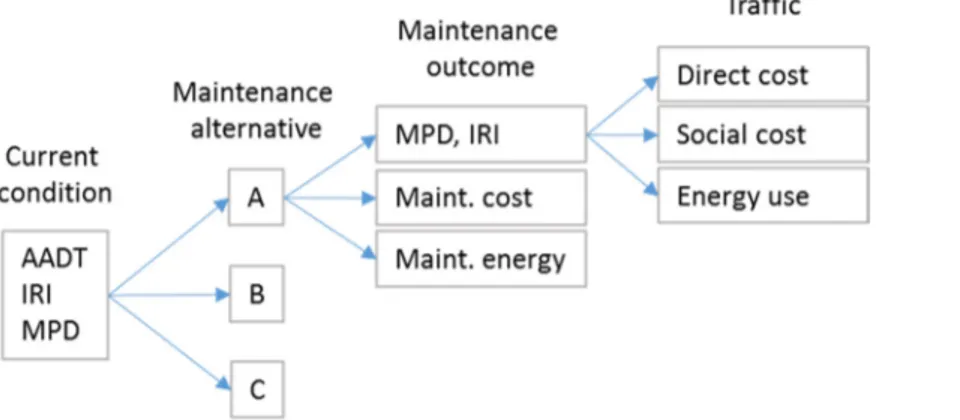
To compare different maintenance alternatives and to decide what strategy to choose; Minimise maintenance cost or minimise energy use, the calculation process described in Figure 1 needs to be amended with the evaluation steps described schematically in Figure 2. The current condition is the same for all alternatives. Each maintenance option leads to its’ specific outcome regarding the road surface conditions, cost and energy use. The resulting surface conditions will in turn have an effect on the cost, both direct and societal, and energy use of the traffic. In each of the steps there are also uncertainties to consider.
Figure 2. Influence diagram showing how current condition will influence decisions and alternatives and finally the resulting outcome.
This report aims at providing a basis for pavement management decision making with respect to total energy and cost, taking into account uncertainties. This basis can be formed by knowledge, procedures and tools. One of these tools could be to have a guideline or a rule of thumb that tells the pavement management if total energy is a relevant issue in a given situation, if the lowering of the rolling resistance through maintenance is efficient enough.
The climate, with rain and snow, will also have an effect on rolling resistance and hence the energy use of traffic. This is to some extent considered in the Winter maintenance management system (WMMS) where it will be possible to calculate and evaluate the most significant impact on road users, road authorities and society of various policies and measures in winter road maintenance. Water prevailing on the road surface is though not considered. Therefore, the presence of water and snow and the effect on traffic fuel consumption during a year will be evaluated.
2.2. Method for the decision procedure
2.2.1. Criteria for cost efficient maintenance that reduces energy
Since the environmental effects of release of CO2 can be valued and compared to other costs. The
relative cost efficiency (Cost Ratio, CR) when comparing two alternatives can therefore be expressed as the difference in total cost (€ Total) divided by the difference in maintenance cost (€ Maint). In other words, if one extra monetary unit cost is used for maintenance, how much is saved in total cost?
Where total cost can be expressed as the sum of maintenance cost and energy related social cost (€ Energy) originating from fuel consumption by traffic and energy used in maintenance.
Which is then formulated as
Where
€ Energy = € Energy_Traffic + € Energy_Maint
€ Energy_Traffic = Direct cost of fuel and environmental cost related to use of fuel. € Energy_Maint = Environmental cost related to use of energy during maintenance. To simplify calculations, it can be assumed that costs are close to those related to the use of diesel only by maintenance and traffic. This means that direct costs of diesel can be used and current pricing of release of CO2, which can be calculated based on carbon content of diesel per litre. The current pricing
in Sweden for direct fuel cost is 14.2 €/GJ and the environmental cost 12 €/GJ, when energy content of diesel (35.1 MJ/litre) is used for normalisation.
2.2.2. Uncertainty and variability and their importance in pavement management
The energy used by traffic can be several orders larger than the energy used during pavementmaintenance. This means that small alterations to evenness and texture may render positive effects on both environment and costs, direct and societal. However, the success of selecting the most beneficial maintenance alternative will be dependent on uncertainties in several steps of the assessment and execution of production. Examples of uncertainties are related to:
Assessment of existing conditions and effects of doing nothing
Assessment of costs and energy use associated with pavement management alternatives. Assessment of pavement condition immediately after maintenance and future development of
pavement condition.
Assessment of energy used and cost associated with traffic as a result of pavement condition. Assessment of future need for maintenance.
Since there are many uncertainties included in the assessment it is inevitable that a certain proportion of pavement sections treated with an ambition to save costs or energy will fail in that respect. On the other hand, if the number of treated sections is very large, even small but significant differences in costs and energy may be worth considering to achieve on average a positive outcome. Two questions then arise:
1. What level of significance is needed and is it important to consider size of objects that will be influenced by decision?
€
€
€
€
€
€
€
€
€
€
1
€
€
€
€
2. Can the level of significance or uncertainty and variability be controlled by pavement management efforts?
The second question is a project on its own, for example, to investigate how procurement and
production can be carried out in such a manner that rolling resistance can be reduced in a cost effective manner.
The first question is of great importance in this report. For large organisations, such as national road administrations, it might be obvious that stochastic variability is of limited interest since there will be an average difference for the road network as a whole that determine how efficient an alternative is. This view is relevant for making policies for road administrations. However, decisions on maintenance alternatives are made on object/project level, where uncertainties are important to consider. Decisions to select one maintenance alternative before another need to be taken based on project level, balancing objectives of agency costs and societal effects such as road user costs and environmental aspects. Balancing decisions against multiple objectives means greater complexity, hence reducing and focusing decisions towards the most important objectives in each particular project and decision situation is beneficial. A suggested procedure is therefore developed that include a step to determine if rolling resistance is an important factor.
2.2.3. Development of decision making procedure
An example is used to describe the development of the decision making procedure. In this example, it is assumed that a road section needs maintenance and that we compare maintenance alternative (1) to alternative (2). For simplicity, assume that alternative (1) is, more or less, a standard alternative and that we need to discuss the best choice in terms of the properties of alternative (2). Once the procedure is defined, none of the alternatives need to be a standard alternative. Also, for further use, the
numbering of the alternatives is arbitrary, i.e. the alternative with the highest cost does not always have to be labelled as alternative (1).
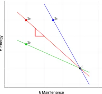
Depending on the difference in price and energy use, we may either prefer alternative (2), find the alternatives equally good or prefer alternative (1). The following procedure will not immediately tell which alternative to use, but it will tell if one should choose with respect to lowest cost or with respect to lowest energy use. A graphic example of the comparison between the alternatives is shown in Figure 3.
If the difference in energy cost is of smaller size than the maintenance cost and of opposite sign, (1) and (2b), the green line, alternative (2) is preferred. (2b) has lower maintenance cost but also higher energy cost. The energy cost is however not so much higher that it cancels out the lower maintenance cost of alternative (1).
The red line, (1) and (2a), are equally good if the difference in maintenance costs is of equal size as the difference in energy cost but with opposite sign. The gain in maintenance cost if changing from an alternative with higher cost to one with lower cost is exactly matched to a loss of equal size in energy cost.
If the difference in maintenance cost is of smaller size than the energy cost and of opposite sign, (1) and (2c), the blue line, alternative (1) is preferred. (2c) has lower maintenance cost but the higher energy cost leads to that alternative (1) is preferred.
As can be seen from this example/figure, for a small negative slope (> -1), alternative (2) is preferred and for high negative slope (< -1), alt (1) is preferred. For a slope near -1 the alternatives are equally good.
Because CR = 1 + slope is means that:
CR > 0 The alternative with lowest maintenance cost is preferred. CR = 0 The alternatives are equal.
CR < 0 The alternative with lowest energy cost is preferred.
CR does not immediately tell which alternative to choose. It tells if the preferred alternative should be chosen according to maintenance cost or to energy cost.
As a note, it is of course possible to create a special case where one alternative has higher maintenance cost and at the same time higher energy cost than the other, meaning that the slope is positive. In that case it is preferred to use the alternative with lower maintenance cost, or the one with lower energy cost, which is in fact the same. Here CR > 1 but the decision rule for CR > 0 gives the correct decision and the decision rules do not need to be changed or completed for this special case.
2.2.4. Uncertainty in the decision
The properties of the variables included in the cost functions should be regarded as random variables. If, for instance, we chose between (1) and (2b) according to what we expect of those alternatives, (2b) is the preferred one. With uncertainty added, the outcome (2-dimensional, maintenance cost and energy cost) acts as one observation in the distribution of possible outcomes. Likewise, the outcome if choosing (1) has a distribution and applying (1) only gives one outcome sampled from that
distribution. Some possible outcomes are shown as bullet clouds in Figure 4. We choose between the alternatives (1) and (2b) according expectations but the result is the random outcome of a comparison between what we should get if we applied (2b) compared to what we should get if we applied (1).
Figure 4. Random outcome of the alternatives (1) and (2b).
With the idea of looking at random outcome, one can connect any pair of one possible outcome of alternative (1) with (2b). Each possible connecting line will have a slope, see Figure 5. This figure shows a sample from the distribution of slopes which can be converted to the distribution of CR. A small proportion of the possible lines have CR < 0 in the example. That is, we choose (2b) based on what we know about the expected maintenance costs but there is a probability that the choice turns out afterwards to not be the best. At some occasions, the random variation makes (2b) having so high energy cost and (1) having so low maintenance cost that (1) would be have been a better choice though 2 was preferred and used. The slopes are shown in Figure 6.
Figure 6. Distribution of slopes between alternative (1) and (2b).
The expected outcome is probably biased, and that may introduce approximations in the decision. Even if expected values of maintenance cost and energy exists together with expected result in IRI and MPD, plugging all these data into the nonlinear CR function does not give exactly the expected CR. Therefore, the decision is probably based on approximately known expected values, the bullets and slopes in Figure 5.
2.2.5. Design of case studies
It was decided that maintenance cost and maintenance energy should have normal distributions and being defined with expected value and standard deviation and correlation 0.25. Also, the outcome in terms of IRI and MPD should have normal distribution with expectation and standard deviation but uncorrelated to each other and to maintenance cost and energy. The expected total energy is approximately found by inserting the expected IRI etc. into a fuel consumption (FC) model (see section 2.4) and then into CR. The decision is then made on that approximation. The distributions of slopes are based on simulation consisting of 100 000 for each comparison.
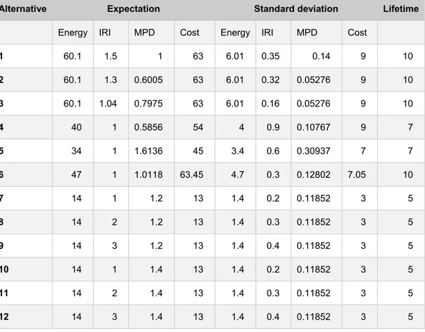
Comparing alternatives with the same expected maintenance cost does not make much sense. Of course one should choose the one with lowest energy in that case. There is though a problem with the equation for CR, that it includes a ratio with a denominator tending to be (at least close to) zero. We did not run any simulation in the case of two alternatives with the same expected maintenance cost. The simulation compared 12 alternatives with each other in pairs, but some pairs are ignored due to equal expected cost. In total, that means we made 48 comparisons between alternatives, but all these were also run with different speeds, ADC, RF and vehicle mix. The alternatives are presented in the table below. Energy in MJ/m2 and cost in SEK/m2. The comparisons refer to a road section that is 1
km long, 8 m wide and with an AADT of 8 000. The length cancels out in CR but must be mentioned to make it possible to interpret mostly what the standard deviations actually represent. The life times are here regarded as fixed without any random variation.
Table 2. Maintenance alternatives with data used in simulations including expected values and standard deviations.
Alternative Expectation Standard deviation Lifetime
Energy IRI MPD Cost Energy IRI MPD Cost
1 60.1 1.5 1 63 6.01 0.35 0.14 9 10 2 60.1 1.3 0.6005 63 6.01 0.32 0.05276 9 10 3 60.1 1.04 0.7975 63 6.01 0.16 0.05276 9 10 4 40 1 0.5856 54 4 0.9 0.10767 9 7 5 34 1 1.6136 45 3.4 0.6 0.30937 7 7 6 47 1 1.0118 63.45 4.7 0.3 0.12802 7.05 10 7 14 1 1.2 13 1.4 0.2 0.11852 3 5 8 14 2 1.2 13 1.4 0.3 0.11852 3 5 9 14 3 1.2 13 1.4 0.4 0.11852 3 5 10 14 1 1.4 13 1.4 0.2 0.11852 3 5 11 14 2 1.4 13 1.4 0.3 0.11852 3 5 12 14 3 1.4 13 1.4 0.4 0.11852 3 5
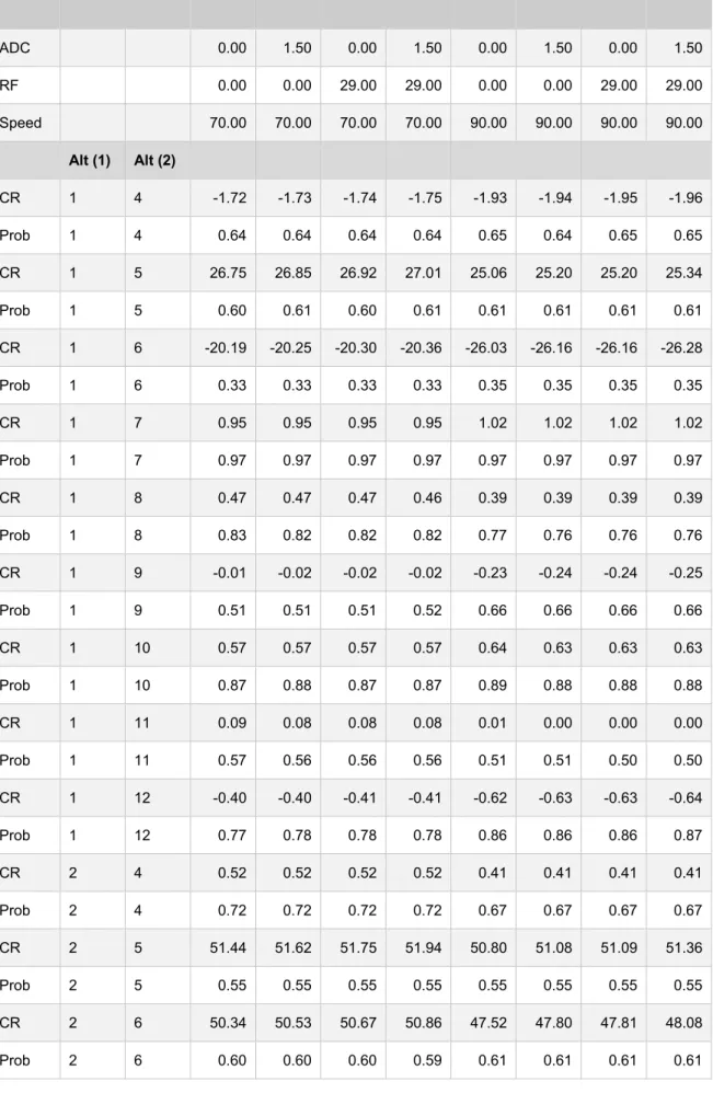
The CR values are approximations with expected values on each of the variables plugged into the fuel consumption model and the following CR calculation. Based on the sign of this value, the decision is made about which alternative is to be preferred (not that at this stage any difference count and the decision cannot be that the alternatives are equal). The Prob values show the probability that the decision becomes correct when uncertainty is introduced.
Table 3. Vehicle mix 96% private cars, 2% trucks, 2% trucks with trailer. ADC 0.00 1.50 0.00 1.50 0.00 1.50 0.00 1.50 RF 0.00 0.00 29.00 29.00 0.00 0.00 29.00 29.00 Speed 70.00 70.00 70.00 70.00 90.00 90.00 90.00 90.00 Alt (1) Alt (2) CR 1 4 -1.72 -1.73 -1.74 -1.75 -1.93 -1.94 -1.95 -1.96 Prob 1 4 0.64 0.64 0.64 0.64 0.65 0.64 0.65 0.65 CR 1 5 26.75 26.85 26.92 27.01 25.06 25.20 25.20 25.34 Prob 1 5 0.60 0.61 0.60 0.61 0.61 0.61 0.61 0.61 CR 1 6 -20.19 -20.25 -20.30 -20.36 -26.03 -26.16 -26.16 -26.28 Prob 1 6 0.33 0.33 0.33 0.33 0.35 0.35 0.35 0.35 CR 1 7 0.95 0.95 0.95 0.95 1.02 1.02 1.02 1.02 Prob 1 7 0.97 0.97 0.97 0.97 0.97 0.97 0.97 0.97 CR 1 8 0.47 0.47 0.47 0.46 0.39 0.39 0.39 0.39 Prob 1 8 0.83 0.82 0.82 0.82 0.77 0.76 0.76 0.76 CR 1 9 -0.01 -0.02 -0.02 -0.02 -0.23 -0.24 -0.24 -0.25 Prob 1 9 0.51 0.51 0.51 0.52 0.66 0.66 0.66 0.66 CR 1 10 0.57 0.57 0.57 0.57 0.64 0.63 0.63 0.63 Prob 1 10 0.87 0.88 0.87 0.87 0.89 0.88 0.88 0.88 CR 1 11 0.09 0.08 0.08 0.08 0.01 0.00 0.00 0.00 Prob 1 11 0.57 0.56 0.56 0.56 0.51 0.51 0.50 0.50 CR 1 12 -0.40 -0.40 -0.41 -0.41 -0.62 -0.63 -0.63 -0.64 Prob 1 12 0.77 0.78 0.78 0.78 0.86 0.86 0.86 0.87 CR 2 4 0.52 0.52 0.52 0.52 0.41 0.41 0.41 0.41 Prob 2 4 0.72 0.72 0.72 0.72 0.67 0.67 0.67 0.67 CR 2 5 51.44 51.62 51.75 51.94 50.80 51.08 51.09 51.36 Prob 2 5 0.55 0.55 0.55 0.55 0.55 0.55 0.55 0.55 CR 2 6 50.34 50.53 50.67 50.86 47.52 47.80 47.81 48.08 Prob 2 6 0.60 0.60 0.60 0.59 0.61 0.61 0.61 0.61
Table 3. (Continued) ADC 0.00 1.50 0.00 1.50 0.00 1.50 0.00 1.50 RF 0.00 0.00 29.00 29.00 0.00 0.00 29.00 29.00 Speed 70.00 70.00 70.00 70.00 90.00 90.00 90.00 90.00 Alt (1) Alt (2) CR 2 7 0.10 0.09 0.09 0.09 0.13 0.12 0.12 0.12 Prob 2 7 0.59 0.59 0.59 0.58 0.61 0.61 0.61 0.60 CR 2 8 -0.39 -0.39 -0.40 -0.40 -0.50 -0.51 -0.51 -0.52 Prob 2 8 0.81 0.81 0.82 0.82 0.85 0.86 0.86 0.86 CR 2 9 -0.87 -0.88 -0.88 -0.89 -1.13 -1.14 -1.14 -1.15 Prob 2 9 0.97 0.97 0.97 0.97 0.99 0.99 0.99 0.99 CR 2 10 -0.28 -0.29 -0.29 -0.30 -0.26 -0.27 -0.27 -0.27 Prob 2 10 0.75 0.75 0.75 0.76 0.72 0.72 0.72 0.73 CR 2 11 -0.77 -0.78 -0.78 -0.79 -0.89 -0.90 -0.90 -0.91 Prob 2 11 0.96 0.96 0.96 0.96 0.97 0.97 0.97 0.97 CR 2 12 -1.25 -1.26 -1.27 -1.28 -1.51 -1.53 -1.53 -1.54 Prob 2 12 1.00 1.00 1.00 1.00 1.00 1.00 1.00 1.00 CR 3 4 -0.13 -0.13 -0.14 -0.14 -0.15 -0.16 -0.16 -0.17 Prob 3 4 0.38 0.39 0.39 0.39 0.40 0.40 0.40 0.40 CR 3 5 44.26 44.42 44.53 44.69 44.57 44.82 44.83 45.06 Prob 3 5 0.55 0.55 0.56 0.56 0.56 0.56 0.56 0.56 CR 3 6 29.83 29.95 30.03 30.14 29.73 29.90 29.91 30.08 Prob 3 6 0.68 0.68 0.68 0.67 0.68 0.68 0.67 0.67 CR 3 7 0.35 0.34 0.34 0.34 0.34 0.34 0.34 0.34 Prob 3 7 0.80 0.80 0.80 0.80 0.79 0.79 0.79 0.79 CR 3 8 -0.14 -0.14 -0.15 -0.15 -0.28 -0.29 -0.29 -0.30 Prob 3 8 0.63 0.63 0.63 0.64 0.74 0.74 0.74 0.75 CR 3 9 -0.62 -0.63 -0.63 -0.64 -0.91 -0.92 -0.92 -0.93 Prob 3 9 0.92 0.92 0.92 0.93 0.97 0.97 0.97 0.97
Table 3. (Continued) ADC 0.00 1.50 0.00 1.50 0.00 1.50 0.00 1.50 RF 0.00 0.00 29.00 29.00 0.00 0.00 29.00 29.00 Speed 70.00 70.00 70.00 70.00 90.00 90.00 90.00 90.00 Alt (1) Alt (2) CR 3 10 -0.04 -0.04 -0.04 -0.05 -0.04 -0.05 -0.05 -0.05 Prob 3 10 0.53 0.54 0.54 0.54 0.54 0.54 0.55 0.55 CR 3 11 -0.52 -0.53 -0.53 -0.54 -0.67 -0.68 -0.68 -0.69 Prob 3 11 0.89 0.89 0.89 0.90 0.93 0.94 0.94 0.94 CR 3 12 -1.01 -1.01 -1.02 -1.02 -1.30 -1.31 -1.31 -1.32 Prob 3 12 0.99 0.99 0.99 0.99 1.00 1.00 1.00 1.00 CR 4 5 -4.57 -4.59 -4.60 -4.62 -4.63 -4.66 -4.66 -4.69 Prob 4 5 0.74 0.74 0.75 0.74 0.73 0.73 0.73 0.73 CR 4 6 -1.11 -1.12 -1.13 -1.13 -1.14 -1.15 -1.15 -1.16 Prob 4 6 0.57 0.57 0.57 0.57 0.55 0.56 0.56 0.56 CR 4 7 0.21 0.21 0.21 0.21 0.21 0.20 0.20 0.20 Prob 4 7 0.67 0.67 0.67 0.66 0.64 0.65 0.64 0.64 CR 4 8 -0.14 -0.14 -0.14 -0.15 -0.25 -0.26 -0.26 -0.26 Prob 4 8 0.61 0.61 0.62 0.62 0.67 0.67 0.67 0.68 CR 4 9 -0.49 -0.49 -0.50 -0.50 -0.70 -0.71 -0.71 -0.72 Prob 4 9 0.84 0.83 0.84 0.84 0.89 0.89 0.89 0.89 CR 4 10 -0.06 -0.07 -0.07 -0.07 -0.07 -0.08 -0.08 -0.09 Prob 4 10 0.55 0.56 0.56 0.56 0.55 0.56 0.56 0.56 CR 4 11 -0.41 -0.42 -0.42 -0.43 -0.53 -0.54 -0.54 -0.54 Prob 4 11 0.80 0.80 0.81 0.81 0.82 0.83 0.83 0.83 CR 4 12 -0.76 -0.77 -0.77 -0.78 -0.98 -0.99 -0.99 -1.00 Prob 4 12 0.94 0.94 0.94 0.94 0.96 0.96 0.96 0.96 CR 5 6 52.03 52.21 52.34 52.52 52.57 52.85 52.86 53.13 Prob 5 6 0.57 0.57 0.57 0.57 0.57 0.57 0.57 0.57
Table 3. (Continued) ADC 0.00 1.50 0.00 1.50 0.00 1.50 0.00 1.50 RF 0.00 0.00 29.00 29.00 0.00 0.00 29.00 29.00 Speed 70.00 70.00 70.00 70.00 90.00 90.00 90.00 90.00 Alt (1) Alt (2) CR 5 7 1.82 1.82 1.83 1.83 1.83 1.83 1.83 1.84 Prob 5 7 0.99 0.99 0.99 0.99 0.99 0.99 0.99 0.99 CR 5 8 1.35 1.35 1.35 1.36 1.22 1.22 1.22 1.22 Prob 5 8 0.96 0.96 0.96 0.96 0.94 0.94 0.93 0.93 CR 5 9 0.88 0.88 0.88 0.88 0.62 0.61 0.61 0.61 Prob 5 9 0.88 0.88 0.87 0.87 0.78 0.77 0.77 0.77 CR 5 10 1.45 1.45 1.45 1.46 1.46 1.46 1.46 1.46 Prob 5 10 0.97 0.97 0.97 0.97 0.97 0.97 0.97 0.97 CR 5 11 0.98 0.98 0.98 0.98 0.85 0.85 0.85 0.85 Prob 5 11 0.91 0.90 0.90 0.90 0.86 0.85 0.86 0.85 CR 5 12 0.51 0.51 0.51 0.51 0.24 0.24 0.24 0.23 Prob 5 12 0.75 0.75 0.75 0.74 0.62 0.62 0.62 0.61 CR 6 7 0.70 0.70 0.70 0.70 0.70 0.69 0.69 0.69 Prob 6 7 0.94 0.94 0.94 0.94 0.93 0.93 0.93 0.93 CR 6 8 0.22 0.22 0.22 0.21 0.08 0.07 0.07 0.07 Prob 6 8 0.69 0.68 0.68 0.68 0.56 0.56 0.56 0.55 CR 6 9 -0.26 -0.26 -0.26 -0.27 -0.54 -0.55 -0.55 -0.56 Prob 6 9 0.70 0.71 0.71 0.71 0.85 0.85 0.86 0.86 CR 6 10 0.32 0.32 0.32 0.32 0.32 0.31 0.31 0.31 Prob 6 10 0.76 0.76 0.76 0.76 0.75 0.74 0.74 0.74 CR 6 11 -0.16 -0.16 -0.16 -0.17 -0.30 -0.31 -0.31 -0.32 Prob 6 11 0.63 0.64 0.63 0.64 0.73 0.73 0.74 0.74 CR 6 12 -0.63 -0.64 -0.64 -0.65 -0.92 -0.93 -0.94 -0.95 Prob 6 12 0.91 0.91 0.91 0.91 0.96 0.96 0.96 0.96
Table 4. Vehicle mix 84% private cars, 8% trucks, 8% trucks with trailer. ADC 0.00 1.50 0.00 1.50 0.00 1.50 0.00 1.50 RF 0.00 0.00 29.00 29.00 0.00 0.00 29.00 29.00 Speed 70.00 70.00 70.00 70.00 90.00 90.00 90.00 90.00 Alt (1) Alt (2) CR 1 4 -3.66 -3.67 -3.68 -3.69 -3.90 -3.91 -3.92 -3.93 Prob 1 4 0.72 0.72 0.72 0.72 0.71 0.71 0.71 0.71 CR 1 5 43.96 44.05 44.15 44.23 39.66 39.79 39.81 39.94 Prob 1 5 0.58 0.58 0.57 0.58 0.58 0.58 0.58 0.58 CR 1 6 -35.54 -35.59 -35.67 -35.72 -44.97 -45.09 -45.13 -45.23 Prob 1 6 0.40 0.40 0.40 0.40 0.41 0.41 0.41 0.41 CR 1 7 0.90 0.90 0.89 0.89 1.02 1.02 1.02 1.02 Prob 1 7 0.88 0.88 0.88 0.88 0.90 0.90 0.90 0.90 CR 1 8 0.01 0.01 0.00 0.00 -0.10 -0.10 -0.10 -0.10 Prob 1 8 0.50 0.51 0.50 0.50 0.54 0.55 0.54 0.55 CR 1 9 -0.88 -0.89 -0.89 -0.89 -1.21 -1.22 -1.22 -1.23 Prob 1 9 0.86 0.86 0.86 0.86 0.92 0.92 0.92 0.92 CR 1 10 0.25 0.25 0.25 0.25 0.39 0.39 0.39 0.39 Prob 1 10 0.63 0.63 0.63 0.63 0.69 0.69 0.69 0.69 CR 1 11 -0.64 -0.64 -0.64 -0.65 -0.73 -0.73 -0.73 -0.74 Prob 1 11 0.79 0.79 0.79 0.79 0.81 0.81 0.81 0.81 CR 1 12 -1.52 -1.53 -1.53 -1.54 -1.84 -1.85 -1.85 -1.86 Prob 1 12 0.97 0.97 0.97 0.97 0.98 0.98 0.98 0.98 CR 2 4 0.16 0.15 0.15 0.15 -0.02 -0.02 -0.02 -0.03 Prob 2 4 0.61 0.60 0.60 0.60 0.43 0.42 0.43 0.43 CR 2 5 85.96 86.14 86.33 86.49 82.31 82.57 82.63 82.88 Prob 2 5 0.54 0.54 0.54 0.54 0.54 0.55 0.54 0.55 CR 2 6 84.47 84.65 84.85 85.02 76.90 77.16 77.21 77.46 Prob 2 6 0.56 0.56 0.56 0.56 0.57 0.57 0.57 0.57
Table 4. (Continued) ADC 0.00 1.50 0.00 1.50 0.00 1.50 0.00 1.50 RF 0.00 0.00 29.00 29.00 0.00 0.00 29.00 29.00 Speed 70.00 70.00 70.00 70.00 90.00 90.00 90.00 90.00 Alt (1) Alt (2) CR 2 7 -0.56 -0.57 -0.57 -0.57 -0.46 -0.47 -0.47 -0.47 Prob 2 7 0.82 0.82 0.82 0.82 0.76 0.76 0.76 0.76 CR 2 8 -1.45 -1.46 -1.46 -1.47 -1.58 -1.59 -1.59 -1.60 Prob 2 8 0.99 0.99 0.99 0.99 0.99 0.99 0.99 0.99 CR 2 9 -2.34 -2.35 -2.35 -2.36 -2.69 -2.71 -2.71 -2.72 Prob 2 9 1.00 1.00 1.00 1.00 1.00 1.00 1.00 1.00 CR 2 10 -1.21 -1.21 -1.22 -1.22 -1.09 -1.10 -1.10 -1.11 Prob 2 10 0.98 0.98 0.98 0.98 0.95 0.95 0.95 0.95 CR 2 11 -2.09 -2.10 -2.11 -2.11 -2.21 -2.22 -2.22 -2.23 Prob 2 11 1.00 1.00 1.00 1.00 1.00 1.00 1.00 1.00 CR 2 12 -2.98 -2.99 -3.00 -3.01 -3.33 -3.34 -3.34 -3.35 Prob 2 12 1.00 1.00 1.00 1.00 1.00 1.00 1.00 1.00 CR 3 4 -0.89 -0.90 -0.90 -0.91 -0.89 -0.89 -0.89 -0.90 Prob 3 4 0.50 0.51 0.50 0.50 0.50 0.50 0.50 0.50 CR 3 5 74.42 74.57 74.73 74.87 72.80 73.02 73.08 73.29 Prob 3 5 0.55 0.55 0.55 0.55 0.55 0.55 0.55 0.55 CR 3 6 51.48 51.59 51.71 51.81 49.72 49.88 49.92 50.07 Prob 3 6 0.61 0.61 0.61 0.61 0.61 0.61 0.61 0.61 CR 3 7 -0.16 -0.17 -0.17 -0.17 -0.13 -0.13 -0.14 -0.14 Prob 3 7 0.61 0.61 0.62 0.62 0.59 0.59 0.59 0.59 CR 3 8 -1.05 -1.06 -1.06 -1.06 -1.25 -1.25 -1.26 -1.26 Prob 3 8 0.96 0.96 0.96 0.96 0.98 0.97 0.98 0.98 CR 3 9 -1.94 -1.95 -1.95 -1.96 -2.36 -2.37 -2.38 -2.39 Prob 3 9 1.00 1.00 1.00 1.00 1.00 1.00 1.00 1.00
Table 4. (Continued) ADC 0.00 1.50 0.00 1.50 0.00 1.50 0.00 1.50 RF 0.00 0.00 29.00 29.00 0.00 0.00 29.00 29.00 Speed 70.00 70.00 70.00 70.00 90.00 90.00 90.00 90.00 Alt (1) Alt (2) CR 3 10 -0.80 -0.81 -0.81 -0.82 -0.76 -0.77 -0.77 -0.77 Prob 3 10 0.92 0.93 0.92 0.93 0.90 0.91 0.91 0.91 CR 3 11 -1.69 -1.70 -1.71 -1.71 -1.88 -1.89 -1.89 -1.90 Prob 3 11 1.00 1.00 1.00 1.00 1.00 1.00 1.00 1.00 CR 3 12 -2.58 -2.59 -2.60 -2.60 -3.00 -3.01 -3.01 -3.02 Prob 3 12 1.00 1.00 1.00 1.00 1.00 1.00 1.00 1.00 CR 4 5 -8.42 -8.44 -8.46 -8.48 -8.25 -8.28 -8.29 -8.32 Prob 4 5 0.76 0.76 0.76 0.76 0.75 0.75 0.75 0.75 CR 4 6 -2.62 -2.62 -2.63 -2.64 -2.55 -2.56 -2.56 -2.57 Prob 4 6 0.66 0.66 0.66 0.66 0.64 0.63 0.63 0.64 CR 4 7 -0.36 -0.37 -0.37 -0.37 -0.34 -0.34 -0.34 -0.35 Prob 4 7 0.68 0.69 0.69 0.69 0.65 0.65 0.65 0.65 CR 4 8 -1.01 -1.01 -1.02 -1.02 -1.15 -1.15 -1.16 -1.16 Prob 4 8 0.90 0.91 0.91 0.91 0.90 0.90 0.90 0.90 CR 4 9 -1.65 -1.66 -1.66 -1.67 -1.96 -1.96 -1.97 -1.97 Prob 4 9 0.98 0.98 0.98 0.98 0.98 0.98 0.98 0.98 CR 4 10 -0.83 -0.83 -0.84 -0.84 -0.80 -0.80 -0.80 -0.81 Prob 4 10 0.86 0.87 0.87 0.87 0.82 0.82 0.82 0.82 CR 4 11 -1.47 -1.48 -1.48 -1.49 -1.60 -1.61 -1.61 -1.62 Prob 4 11 0.97 0.97 0.97 0.97 0.96 0.96 0.96 0.96 CR 4 12 -2.12 -2.12 -2.13 -2.13 -2.41 -2.42 -2.42 -2.43 Prob 4 12 1.00 1.00 1.00 1.00 1.00 1.00 1.00 1.00 CR 5 6 86.77 86.94 87.13 87.29 85.23 85.49 85.55 85.80 Prob 5 6 0.55 0.55 0.55 0.55 0.55 0.55 0.55 0.55
Table 4. (Continued) ADC 0.00 1.50 0.00 1.50 0.00 1.50 0.00 1.50 RF 0.00 0.00 29.00 29.00 0.00 0.00 29.00 29.00 Speed 70.00 70.00 70.00 70.00 90.00 90.00 90.00 90.00 Alt (1) Alt (2) CR 5 7 2.34 2.34 2.35 2.35 2.32 2.32 2.32 2.33 Prob 5 7 0.97 0.97 0.97 0.97 0.97 0.97 0.97 0.97 CR 5 8 1.48 1.48 1.49 1.49 1.24 1.24 1.24 1.24 Prob 5 8 0.89 0.89 0.89 0.89 0.83 0.83 0.83 0.83 CR 5 9 0.62 0.62 0.62 0.62 0.16 0.16 0.16 0.16 Prob 5 9 0.70 0.69 0.69 0.69 0.55 0.55 0.55 0.55 CR 5 10 1.72 1.72 1.72 1.73 1.71 1.71 1.71 1.71 Prob 5 10 0.92 0.92 0.92 0.92 0.91 0.91 0.91 0.91 CR 5 11 0.86 0.86 0.86 0.86 0.63 0.63 0.63 0.63 Prob 5 11 0.76 0.76 0.76 0.76 0.69 0.69 0.69 0.69 CR 5 12 0.00 0.00 0.00 0.00 -0.45 -0.45 -0.46 -0.46 Prob 5 12 0.50 0.50 0.50 0.50 0.63 0.63 0.64 0.64 CR 6 7 0.46 0.46 0.46 0.45 0.47 0.47 0.47 0.46 Prob 6 7 0.75 0.75 0.74 0.75 0.74 0.74 0.74 0.74 CR 6 8 -0.42 -0.42 -0.43 -0.43 -0.63 -0.64 -0.64 -0.65 Prob 6 8 0.72 0.72 0.72 0.72 0.80 0.80 0.80 0.80 CR 6 9 -1.30 -1.30 -1.31 -1.31 -1.74 -1.75 -1.75 -1.76 Prob 6 9 0.96 0.96 0.96 0.96 0.98 0.98 0.98 0.98 CR 6 10 -0.18 -0.18 -0.18 -0.18 -0.15 -0.16 -0.16 -0.16 Prob 6 10 0.60 0.60 0.60 0.61 0.59 0.59 0.59 0.59 CR 6 11 -1.05 -1.06 -1.06 -1.07 -1.26 -1.26 -1.27 -1.27 Prob 6 11 0.93 0.93 0.93 0.93 0.95 0.95 0.95 0.95 CR 6 12 -1.93 -1.94 -1.94 -1.95 -2.36 -2.37 -2.37 -2.38 Prob 6 12 0.99 1.00 1.00 1.00 1.00 1.00 1.00 1.00
2.3. Climate
Both snow and water on the road surface will influence the rolling resistance and hence the fuel use. This is due to the need to displace an amount of snow or water in front of the wheel and the size of this extra force is dependent on the volume to displace and also the density in the case of snow.
In Table 5 the climate data retrieved for the two case studies in Karlsson et al.. (2012) is presented. The data is retrieved from RWiS (Road Weather information System) outstations that are nearby the road sections. The data is for October 15 2004 to April 15 2005 and this year was chosen because the precipitation was close to normal (based on statistics 1961–1990). The number of hours with rain or snow fall can be seen for each outstation.
Table 5. Distribution of road surface condition. Number of hours and percentage of time in the winter of 2004/2005.
Case E20 Case RV47 hours % of time hours % of time
Wet road 153 3% 274 6% Snowy road 360 8% 315 7% No precipitation 88% 87%
For the calculations of the amount of time the road surface is covered with water or moist, two sub-models of the VTI Winter Model1 are used, “Splashing from a wet road” and “Drying of a moist
road”. The first sub-model describes the variables that control the water disappearing from the road. Significant variables are traffic flow, the ratio between the number of cars and trucks, speed, wind speed and direction, road gradient and texture. This sub-model is used as long as the road is described as wet (>10 g/m2), and when the road turns to be moist the second model take over. In this
sub-model calculations are done of the transition from moist to dry surface through evaporation. The parameters taken into account are: road surface temperature, dew point temperature and wind speed, but also traffic flow, the ratio between the number of cars and trucks, speed, and salinity in the moisture.
To evaluate the effect on fuel use due to the presence of water and snow on the road surface the traffic simulation model VETO has been used (see section 2.4). In the evaluation, the amounts of snow and water on the road are varied and the resulting fuel use is compared to a situation with a dry road surface conditions. For dry road surface, fuel use has been estimated for each vehicle categories used in the case studies, with three different outdoor temperatures and with different combinations of IRI and MPD. The estimated fuel use when there is snow or water present on the road surface are presented as relative values, in %, the reference values of a dry road.
The type of snow is altered by using different densities, see Table 6. The densities for the various snow types are defined as intervals (Hjort 2012) and the ones that are used in the calculations are the mid value within each interval. Also, there is a possibility in VETO to define the percentage of how
1 VINTER is a model for winter maintenance strategies of roads and deals with the effects on accidents,
accessibility (speeds and flows), fuel consumption, corrosion, environmental effects, the costs incurred by the road administration for the measures, and the costs of the road administration for wear.
much the first axle of the vehicle are exposed to the snow and water depth respectively. For snow, this has been studied for 100% and 25%, and for water 100% is used.
Table 6. Type of snow and the density.
Type of snow Density
[kg/m3] Density used in the estimations
[kg/m3]
New 50-200 125
Powder 500-450 325
Wet 300-700 500
Compact 450-700 575
The yearly average ambient air temperature is set to 8˚C for the whole year and is used for estimations of fuel use due to water on the road surface. During wintertime and for the evaluation of snow, the temperature is set to 1.5˚C and this represents the average temperature during winter (Nov.–Feb.) in the region where the three roads are situated. To see if the temperature will have an impact, the fuel use during a temperature -5˚C was also estimated for snow.
Three roads are used for the case study. One road, called MW, represents a 1 km 2+2 lane motorway with a speed limit of 110 km/h and where the road in each direction is 13 m wide. The second
represents a 1 km 1+1 lane rural road with a speed limit of 90 km /h, called RUR_90, with a width of 9 m. These two roads are straight and flat, i.e. both geometrical and vertical alignment is set to 0. The third example is a small rural road with a speed limit of 70 km/h and a width of 6 m. This road is named RUR_70 and it has more curvature and rise and fall than the other two examples. For RUR_70, the geometrical and vertical alignment vary in the estimations throughout the studied stretch.
The IRI and MPD for dry and wet roads are combined using the following values: IRI: 1.0; 1.5; 2.0; 2.5; 3.0; 3.5; 4.0
MPD: 0.5;1.0; 1.5; 2.0
Regarding snowy roads, IRI is varied along with the characteristics of the snow. MPD is in these cases automatically set to 0.5 by VETO. The investigated depth of snow is 1 to 5 cm with 1 cm step, and for water the depths are 0.5 mm, 1mm and up to 7 mm with 1 mm step. These estimations are made the roads and four vehicle types; passenger cars (petrol and diesel), truck and truck with trailer. In total 5 670 estimations of fuel use are calculated.
2.4. VETO
VETO is a simulation model, which can be used to estimate fuel consumption of traffic due to various characteristics of vehicles, roads and driving behaviour. It is a mechanistic model based on physical relationships in which it is possible to describe both vehicles and specific road segments with high precision (Hammarström, Karlsson 1987).
The basic data in VETO consists of the following main parts:
Vehicle: Details about the vehicle such as type of vehicle, air resistance, weight, engine power, fuel type, engine fuel map, tyres and transmission.
Driving behaviour: Speed can be defined as a function of road width. With gear change one can define the use of max torque during acceleration and for steady state speed, deceleration and gear change decisions.
Weather: Wind speed, special wind angles, air temperature, air pressure, water depth, and snow depth and density.
The various input parameters can be changed to investigate vehicles energy under different conditions.
VETO has been used to derive the fuel consumption function (Fcs) that is included in the criterion used to choose maintenance alternative. In Hammarström et al. (2012) the Fcs was developed for free flow situation, assuming typical vehicle data, conditions and driving patterns using models
implemented in VETO. The function is defined as:
1 1 5 1 2 3
where:
Fcs: Fuel use [liter/10 km]
Fr: Rolling resistance 0 1 2
Fair: Air resistance ⁄ 2
v: vehicle speed [m/s]
ADC: road curvature [rad/km]
RF: slope [m/km]
IRI: Road roughness [m/km]
MPD: Macrotexture [mm]
m: Mass [kg]
g: Standard gravity [m/s2]
Cd: Air dynamic coefficient
A: Projected front area of the vehicle [m2]
dns: Air density [kg/m2]
c1, k5, d1, d2, d3, Cr0, Cr1, Cr2: Parameters, values vary with vehicle type.
VETO has also been used to evaluate fuel use due to the presence of snow and water on the road surface. The vehicles and driving behaviour represent typical Swedish conditions. The fuel use in dm3/10 km is estimated for one type of vehicle according to the defined parameters in the model. To
calculate the expected fuel use for one year, the figure in dm3/10 km for each vehicle type is
transformed to MJ/(km road section) and multiplied with the AADT for the specific vehicle type. The energy use for the different vehicle types are added together to get the total yearly traffic energy use for the road section in the case study.
3.
Statistical analysis
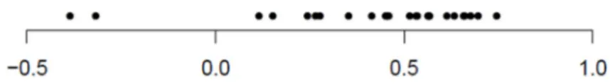
A decision quarter circle is presented in Figure 7. When comparing altenatives, represented by the red and one of the black dots, a CR value is found. The decision circle shows, for different CR values, how the alternatives compare to each other. The CR value and the decision strategy (choose according to energy (E), to cost (C) or being undecisive(U)) are shown for some examples. CR is not calculated for the alternative at “12 o’clock” because CR is not mathematically defined in this point (division by zero).
The figure does not show a complete circle since the CR and decision rule will be the same on the opposite side of any of the shown examples. Problems arise mostly when two alternatices around “12 o’clock” are compared because in that case one should choose according to energy (E) but the slope, and CR can jump between high negative and high positive values after only very small change in cost.
Figure 8. Different cases with two maintenance alternatives in each giving a difference in energy cost and maintenance cost.
The six cases shown in Figure 8 describe possible outcomes and how they can be interpreted. These have been selected as examples with different properties, but of course the outcomes are not limited to only these.
A. The two maintenance alternatives have almost equal expectation of cost and also of energy. It is not possible to recommend one maintenance method over the other. The main uncertainty depends on the variation between outcomes of the same alternative but not on the difference between alternatives.
B. The methods have different expected cost but almost the same expected energy. It is probably best to choose the one with lowest cost, but it is an uncertain decision. For the majority of combinations of one read and one black bullet, the red bullet has a better position in the cost/energy-plane, but the probability of making “wrong” decision cannot be neglected. C. The two alternatives are clearly separated in cost and in energy, but deciding which one is the
with is expected to almost exactly compensate for the cost. Though the alternatives are separated, the effect of choosing one over the other is unclear. When combining one red and one black bullet, it is only random if it will be more or less steep than the decision line. D. The alternatives have almost exactly the same expected cost but quite different energy
demand. The slope, when combining a red and a black bullet, varies randomly between a high negative and a high positive slope. CR does not clearly support which decision to make but after seeing the figure it is clear that one should choose the alternative with lowest energy demand.
E. The alternatives are clearly separated. In this case, CR shows that the decision strategy must be to choose according to energy.
F. Most combinations of a red and a black bullet shows that it is better to choose according to cost but the alternatives have different variation in energy demand The decision can be better supported of one could first of all reduce the uncertainty in the energy dimension for the alternative represented by black bullets.
The six cases above are also noted with the corresponding letter in the tables presenting simulation results in Appendix 1.
4.
Climate
In this section, the effect on fuel use due to the presence of snow or water on the road surface is presented. The impact of snow and water is described as relative values in percent of dry road conditions and where the MPD = 1.0 in the case of water. The different roads are shortly described in 2.3.
For a complete list of the effect of water and snow see Appendix 2 and Appendix 3.
4.1. Dry road conditions
In Table 7 to Table 9, and in Figure 9, the absolute values of estimated fuel use for the different vehicle categories and at different IRI and MPD for the three roads in the case studies are presented. As can be seen, the fuel use is in general higher the higher the IRI, MPD and speed. One difference to this can be found for RUR_70, where the fuel use for trucks with trailer greatly differs from the fuel use on MW and RUR_90. This is due to that RUR_70 has more difference in vertical and horizontal alignment whereas MW and RUR_90 are flat and straight. This curvature leads to a driving behaviour that is not as smooth as for a flat and straight road, with more accelerations and breaking which will have a direct influence on fuel use. Also, the RUR_70 represents a road where trucks with trailers normally do not drive and therefore this alternative is left out in the results from here on.
Table 7. Fuel use for Passenger cars (petrol) at different IRI and MPD. Roads MW, RUR_90 and
RUR_70. [dm3/10km].
Passenger car (petrol)
MW RUR_90 RUR_70 IRI MPD=0.5 MPD=2.0 MPD=0.5 MPD=2.0 MPD=0.5 MPD=2.0 1.0 0.711 0.737 0.600 0.628 0.472 0.487 1.5 0.714 0.740 0.603 0.631 0.473 0.488 2.0 0.717 0.743 0.606 0.634 0.474 0.489 2.5 0.721 0.747 0.609 0.637 0.475 0.490 3.0 0.724 0.750 0.612 0.640 0.476 0.491 3.5 0.727 0.753 0.615 0.642 0.477 0.492 4.0 0.730 0.756 0.618 0.645 0.478 0.493
Table 8. Fuel use for Trucks at different IRI and MPD. Roads MW, RUR_90 and RUR_70. [dm3/10km]. Trucks no trailer MW RUR_90 RUR_70 IRI MPD=0.5 MPD=2.0 MPD=0.5 MPD=2.0 MPD=0.5 MPD=2.0 1.0 2.291 2.408 2.077 2.206 1.910 1.892 1.5 2.307 2.424 2.094 2.222 1.908 1.896 2.0 2.322 2.439 2.110 2.237 1.868 1.899 2.5 2.338 2.453 2.126 2.253 1.874 1.902 3.0 2.353 2.468 2.143 2.269 1.876 1.910 3.5 2.369 2.482 2.159 2.285 1.878 1.913 4.0 2.385 2.497 2.175 2.300 1.889 1.914
Table 9. Fuel use for Trucks with trailer at different IRI and MPD. Roads MW, RUR_90 and RUR_70. [dm3/10km].
Trucks with trailer
MW RUR_90 RUR_70 IRI MPD=0.5 MPD=2.0 MPD=0.5 MPD=2.0 MPD=0.5 MPD=2.0 1.0 3.424 3.815 3.355 3.732 5.078 5.109 1.5 3.467 3.864 3.395 3.780 5.084 5.228 2.0 3.509 3.913 3.436 3.827 5.088 5.224 2.5 3.556 3.963 3.476 3.875 5.098 5.226 3.0 3.605 4.013 3.516 3.923 5.099 5.227 3.5 3.655 4.062 3.562 3.971 5.166 5.228 4.0 3.704 4.112 3.611 4.020 5.169 5.230
Figure 9. Example of fuel use during dry road conditions of different vehicle categories and roads. IRI = 1.0 to 4.0 and MPD = 1.0.
4.2. Water
In Figure 10 to Figure 12, examples of VETO simulation results for fuel use at different water film thickness on the road surface are presented.
Figure 10. Example of fuel use relative a dry road, MW, Truck with trailer. Different water film thickness. IRI = 1.0 to 4.0, MPD = 1.0.
As can be seen in Figure 10, the relative fuel use is fairly constant for the different IRI and for most water depths. A slightly negative slope can be noticed, which means that the importance of water on the road surface is decreasing with an increase in IRI, i.e. a high IRI is more dominant in regards of the impact on fuel use. This is especially visible where the water depth is 5 mm. Between an IRI of 2.5 and 3 there is a shift. This is to some extent also explained by that the increased resistance will lead to a reduction in speed that will further reduce the relative difference to a dry road surface.
Figure 11. Example of fuel use relative a dry road, RUR_90, Truck. Different water film thickness. IRI = 1.0 to 4.0, MPD = 1.0.
At a water depth of 3 mm, the speed is lower relative the alternatives with less water. This has an influence on the fuel use, which is shown in the presence of indents in the fuel use curve. This is also the case with 4 and 5 mm water, where the increased rolling resistance is offset by a lower speed. As also can be seen in Figure 11, the relative fuel use has a somewhat negative slope for all water depths. The absolute fuel use does increase with a higher IRI but the relative fuel use, i.e. the difference between a dry and wet road surface decreases.
F uel use, r elat iv e dry road and MPD=1. 0
Figure 12. Example of fuel use relative a dry road, RUR_70, Passenger car (petrol). Different water film thickness. Fuel use relative a dry road. IRI = 1.0 to 4.0 and MPD = 1.0.
For a passenger car on a RUR_70, the relative fuel use is fairly constant for the different IRI. As can be expected it is relatively larger the more water on the road surface since it affects the rolling resistance. However, the change in fuel use gets smaller for each extra mm thickness which to some extent is explained by a slight decrease in speed.
4.3. Snow
When simulating the level of snow on the roads, the value of MPD of the road surface is not important since the snow is assumed to cover the macrotexture. Figure 13 to Figure 15 is examples of the impact on fuel use due to snow on the road surface with regards to different snow densities, snow depth and 1st axle exposure to the snow.
Figure 13. Example of fuel use relative a dry road. MW, Truck with trailer. Different snow densities, snow depth and 1st axle exposure. IRI = 1.0
Figure 14. Example of fuel use relative a dry road. RUR_90, Truck. Different snow densities, snow depth and 1st axle exposure. IRI = 2.0
Figure 15. Example fuel use relative a dry road. RUR_70, Passenger car (petrol). Different snow densities, snow depth and 1st axle exposure. IRI = 2.0
One difference between the various vehicle categories is that passenger cars seems to be relatively more sensitive to snow in regards to the extra fuel use needed to overcome the increased rolling resistance. Especially, with the assumption of 100% exposure to the snow depth of the first axle.