APPLICATION OF NATIONWIDE WEATHER DATA FOR TRAFFIC
SAFETY ANALYSIS IN THE UNITED STATES: A SPATIAL ANALYSIS
AND CRASH PREDICTION MODELING
Whoibin Chung University of Central Florida
4000 Central Florida Blvd, Orlando, United states Phone: +1 407-823-0300 E-mail: jwhoibin@knights.ucf.edu
Co-authors(s); Mohamed Abdel-Aty, University of Central Florida; Keechoo Choi, Ajou University; Jaeyoung Lee, University of Central Florida
1.
INTRODUCTION
There has been a wide range of scientific research to investigate the effects of adverse weather on traffic safety. In particular, some researchers have analyzed the relationship between traffic crash occurrence and weather condition in the United States using the data from land-based weather stations. Using traffic crash and weather data throughout the United States, Eisenberg (2004) analyzed the mixed effects of precipitation, and Eisenberg and Warner (2005) investigated the impact of snowfall. In addition, Ashley et al. (2015) dealt with a nationwide analysis of visibility-related fatal crashes in the United States and Black and Mote (2015) conducted a spatial and temporal analysis of winter-precipitation-related fatal crashes.
Different from the previous research, this paper investigates the effective spatial coverage of nationwide land-based weather stations of the National Oceanic Atmospheric Administration (NOAA) for traffic crash analysis. Based on the effective spatial coverage, statistical models by the United States climate regions were developed to confirm whether the weather data within the coverage could be a good exposure measure for traffic crash analysis.
2.
ANALYSIS METHOD
2.1. Contingency table analysis
To investigate the effective spatial coverage of weather stations, contingency tables by 5, 10, 15, and 20 miles were created. As assessment measures, sensitivity, positive predictive values (PPV), and Cohen’s Kappa were compared by the coverage. The Kappa can be estimated as follows:
𝜅 =𝑜𝑏𝑠𝑒𝑟𝑣𝑒𝑑 𝑎𝑔𝑟𝑒𝑒𝑚𝑒𝑛𝑡 − 𝑐ℎ𝑎𝑛𝑐𝑒 𝑎𝑔𝑟𝑒𝑒𝑚𝑒𝑛𝑡
1 − 𝑐ℎ𝑎𝑛𝑐𝑒 𝑎𝑔𝑟𝑒𝑒𝑚𝑒𝑛𝑡 =
𝑃𝑜− 𝑃𝑐
1 − 𝑃𝑐
The Kappa statistic is interpreted as the strength of agreement: <0.00=poor, 0.00-0.20=slight, 0.21-0.40=fair, 0.41-0.60=moderate, 0.61-0.80=substantial, and 0.81-1.00=almost perfect (Landis & Koch, 1977).
2.2. Crash prediction modeling
To assess the applicability of weather data within the effective spatial coverage of weather stations as a good exposure, a series of negative binomial regression models were developed. The first type of models relates total fatal crashes under specific weather conditions to the annual total length of the corresponding weather as follows:
𝑙𝑛𝜆𝑖 = 𝛽0+ 𝛽1ln (𝑉𝑀𝑇𝑖∗ 𝐷𝑢𝑟𝑎𝑡𝑖𝑜𝑛𝑖)
where 𝜆𝑖 is the expected fatal crash counts for a given observation within the specific radius from
weather station i; 𝑉𝑀𝑇𝑖 is the multiplication of AADT and segment length within station i; and
𝐷𝑢𝑟𝑎𝑡𝑖𝑜𝑛𝑖 is the annual total length of rain, snow, and fog at weather station i.
The second type of models investigates the relationship between annual total fatal crashes and duration of each weather condition as follows:
𝑙𝑛𝜆𝑖= 𝛽0+ 𝛽1𝑙𝑛𝑉𝑀𝑇𝑖+ 𝛽2𝑅𝑎𝑖𝑛𝑖+ 𝛽3𝑆𝑛𝑜𝑤𝑖+ 𝛽4𝐹𝑜𝑔𝑖
where 𝑅𝑎𝑖𝑛, 𝑆𝑛𝑜𝑤, 𝑎𝑛𝑑 𝐹𝑜𝑔 are the annual total duration of each weather condition.
3.
DATA PREPARATION
The data were collected from three sources: 1) Weather data from the NOAA’s QCLCD (Quality Controlled Local Climatological Data) during May 2007 to December 2014; 2) Fatal crash data from NHTSA’s Fatality Analysis Reporting System (FARS) during 2007 to 2014; and 3) annual average daily traffic from the Federal Highway Administration’s Highway Performance Monitoring System (HPMS) during 2011 to 2012
The QCLCD is representative qualified nationwide weather data collected from 2,466 weather stations including AWOS (Automated Weather Observing System), MAPSO (Microcomputer-Aided Paperless Surface Observations), Navy METAR (METeorological Aerodrome Report), ASOS (Automated Surface Observing System), CRN (Climate Reference Network) and so on.
3.1. Contingency tables
One weather data set was prepared by combining all QCLCD of all years and cleaning weather stations with no data. Fatal crash data sets were prepared using fatal crashes extracted within the radius of coverages such as 5, 10, 15, 20 miles on the basis of the weather station locations. Using the weather stations and recorded times, two data sets were joined and finally the corresponding weather conditions were compared each other.
3.2. Statistical modeling
VMT were prepared using AADT and its segment length extracted within the radius of coverages such as 5, 10, 15, 20 miles on the basis of the weather station locations. Annual time period of each weather condition was aggregated from the prepared weather data set.
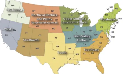
3.3. USA Climate Regions
Based on nine climate regions, which were classified by Karl and Koss (1984), cumulative observation duration of rain, snow, and fog were aggregated to look into regional characteristics.
Figure 2. USA Climate Regions (Source: https://www.ncdc.noaa.gov/monitoring-references/maps/us-climate-regions.php)
4.
RESULTS
4.1. Contingency table analysis
According to the contingency table analysis results, sensitivity, PPV, and Cohen’s Kappa decrease a little as the coverage is extended, but the reduction is within 1 and 2 percent. The sensitivity is high in the order of fog, snow, and then rain. In the case of PPV, rain and snow weather conditions have PPV more than 65%, but fog has extremely low PPV of less than 10%. Likewise, Cohen’s Kappa of each weather condition showed that rain and snow have a moderate agreement but fog has a slight agreement. In terms of overall Cohen’s Kappa, QCLCD has a moderate agreement with FARS.
Sensitivity PPV
Cohen’s Kappa of each weather condition Overall Cohen’s Kappa Figure 3. Contingency Table Analysis Results
4.2. Negative Binomial Regression Model
For most regions, the increase of VMT during specific weather duration has a significant positive relationship with weather-related fatal crashes. This result also confirms the feasibility of the QCLCD for traffic safety analysis as the sensitivity and positive predicted values verified in the previous section. Table 1. Negative binomial model of regional annual fatal crash frequency by each weather condition
Climate
Region Variable
Clear/Cloud Rain Snow Fog
Coefficient p-value Coefficient p-value Coefficient p-value Coefficient p-value Central Intercept -5.1631 <.0001 0.6860 0.0043 -2.0451 0.0005 -1.2887 0.0041 ln (VMT*D) 0.4633 <.0001 0.07498 <.0001 0.1582 <.0001 0.06719 0.0101 𝛼 0.2868 0.8528 0.4676 0.0055 0.00005 East North Central Intercept -9.5490 <.0001 -1.7720 <.0001 -1.8041 <.0001 -3.2652 <.0001 ln (VMT*D) 0.6513 <.0001 0.1636 <.0001 0.1347 <.0001 0.1541 0.0012 𝛼 0.3717 1.8544 0.6683 0.6577 North-east Intercept -4.9785 <.0001 1.5238 <.0001 0.002112 0.9908 -0.6333 0.0089 ln (VMT*D) 0.4663 <.0001 0.05913 <.0001 0.03381 0.0064 *0.02586 0.0769 𝛼 0.6212 0.9290 0.3844 0.3726 North-west Intercept -9.1769 <.0001 0.3731 0.2754 -1.7548 0.0037 -1.6099 0.0035 ln (VMT*D) 0.6273 <.0001 0.06815 0.0014 0.08459 0.0422 0.06932 0.0400 𝛼 0.4152 1.9388 1.996E-7 0.2244 South Intercept -8.0777 <.0001 0.2673 0.1539 -3.6732 <.0001 -1.5394 <.0001 ln (VMT*D) 0.6084 <.0001 0.06623 <.0001 0.1526 0.0200 0.06508 0.0025 𝛼 0.4152 1.2223 1.1733 1.4359 South-east Intercept -4.9149 <.0001 0.8522 <.0001 -5.2586 <.0001 -1.3640 <.0001 ln (VMT*D) 0.4611 <.0001 0.06573 <.0001 0.2379 0.0021 0.07869 <.0001 𝛼 0.4769 0.6116 2.4132 0.2949 South-west Intercept -7.3319 <.0001 -1.1484 0.0012 -2.4865 <.0001 -12.1799 <.0001 ln (VMT*D) 0.5706 <.0001 0.08783 0.0009 0.1470 <.0001 0.6636 <.0001 𝛼 1.0355 3.4204 <.0001 1.5607 3.333E-6 West Intercept -6.3014 <.0001 0.01858 0.9562 -4.1764 <.0001 -6.1521 <.0001 ln (VMT*D) 0.5411 <.0001 0.1198 <.0001 0.2034 0.0016 0.3724 <.0001 𝛼 0.8809 1.7348 1.8565 0.1770 West North Central Intercept -9.6524 <.0001 -1.5738 0.0054 -1.2109 0.0144 -7.8874 <.0001 ln (VMT*D) 0.6329 <.0001 #0.04819 0.2292 #0.008660 0.8128 0.3913 <.0001 𝛼 0.3489 0.9159 1.3443 0.1191 1.011E-7 Note:
D means the average annual duration of each weather condition. # indicates that the variable is not significant at 10% level.
* indicates that the variable is significant only at 10% level, and all other variables are significant at 5% level.
The results in Table 2 shows that there are no meaningful weather effects on fatal crashes in the Central region. The rain weather has a significant positive relationship with fatal crashes in East North, Northeast, Northwest, South, and West North Central in contrast with the West region. The snow weather has a significant negative relationship with fatal crashes in the East North Central, Northeast, Southeast, West, and West North Central regions. While the fog weather has no significant association with fatal crashes in most regions, it has the significant negative relationship with regional fatal crashes in the Northwest and Southwest, and it has a significant positive correlation in the West at 10% significance level.
Table 2. Regional feature between total fatal crashes and duration of each weather condition
Central East North Central Northeast
Variables Coefficient p-value Coefficient p-value Coefficient p-value
Intercept -4.4562 <.0001 -8.0054 <.0001 -4.0116 <.0001 ln (VMT) 0.4404 <.0001 0.5705 <.0001 0.4244 <.0001 % of rain duration - - 0.02770 <.0001 0.009015 0.0018 % of snow duration - - -0.02439 <.0001 -0.03060 <.0001 % of fog duration - - - - 𝛼 0.3191 0.2561 0.3966
Northwest South Southeast
Variables Coefficient p-value Coefficient p-value Coefficient p-value
Intercept -8.3583 <.0001 -7.7137 <.0001 -4.3752 <.0001 ln (VMT) 0.5920 <.0001 0.5950 <.0001 0.4496 <.0001 % of rain duration 0.007762 0.0022 0.01028 0.0074 - - % of snow duration - - -0.08391 <.0001 -0.07796 <.0001 % of fog duration -0.00412 0.0207 - - - - 𝛼 0.3280 <.0001 0.3936 <.0001 0.3930 <.0001
Southwest West West North Central
Variables Coefficient p-value Coefficient p-value Coefficient p-value
Intercept -7.3920 0.7422 -6.1194 <.0001 -10.0059 <.0001 ln (VMT) 0.5902 0.04040 0.5503 <.0001 0.6546 <.0001 % of rain duration - - -0.02573 <.0001 0.03622 <.0001 % of snow duration - - -0.03812 <.0001 -0.02722 0.0009 % of fog duration -0.02535 0.006901 0.003522 0.0609 - - 𝛼 0.9055 <.0001 0.6420 <.0001 0.2745 <.0001
5.
CONCLUSION
By using the nationwide QCLCD including various types of land-based weather stations, it was confirmed what spatial coverage of weather stations is effective and that weather data within the effective coverage are a good exposure for the prediction of traffic crash. According to the estimated Cohen’s κ statistics, the rain and snow weather conditions have a moderate agreement up to 20 miles. However, in the case of fog weather condition, it has a slight agreement. The statistical modeling results showed that weather station data could be a good exposure measure for weather-related fatal crashes along with the vehicle-miles-traveled. Considering that approximately more than 75% of all fatal crashes are located within 20-miles radius of the weather stations in the United States, it is evident that the data from the land-based weather stations can be cost-effective to develop geospatial crash risk model considering the effects of weather conditions.
REFERENCES
Ashley, W. S. et al. (2015). Driving blind: Weather-related vision hazards and fatal motor vehicle crashes. Bulletin of the American Meteorological Society, 96(5), p. 755-778.
Black, A. W., & Mote, T. L. (2015). Characteristics of winter-precipitation-related transportation fatalities in the United States. Weather, climate, and society, 7(2), p. 133-145.
Eisenberg, D. (2004). The mixed effects of precipitation on traffic crashes. Accident analysis & prevention, 36(4), p. 637-647.
Eisenberg, D., & Warner, K. E. (2005). Effects of snowfalls on motor vehicle collisions, injuries, and fatalities. American Journal of Public Health, 95(1), p. 120-124.
Karl, T., & Koss, W. J. (1984). Regional and national monthly, seasonal, and annual temperature weighted by area, 1895-1983: National Climatic Data Center.
Landis, J. R., & Koch, G. G. (1977). The measurement of observer agreement for categorical data. biometrics, p. 159-174.