Research
2010:46
Development of the PRO-LOCA
Proba-bilistic Fracture Mechanics Code,
MERIT Final Report
Authors: Paul Scott Robert Kurth Andrew Cox Rick Olson Dave Rudland
Title: : Development of the PRO-LOCA Probabilistic Fracture Mechanics Code, MERIT Final Report. Report number: 2010:46
Author: Paul Scott1), Robert Kurth1), Andrew Cox1), Rick Olson1) and Dave Rudland2) 1)Battelle Columbus, USA , 2)Nuclear Regulatory Commission, USA.
Date: December 2010
This report concerns a study which has been conducted for the Swedish Radiation Safety Authority, SSM. The conclusions and viewpoints presented in the report are those of the authors and do not necessarily coincide with those of the SSM.
Background
The MERIT project has been an internationally financed program with the main purpose of developing probabilistic models for piping failure of nuclear components and to include these models in a probabilistic code named PRO-LOCA.
Objectives of the project
The principal objective of the project has been to develop probabilistic models for piping failure of nuclear components and to include these models in a probabilistic code.
Results
The MERIT program has produced a code named PRO-LOCA with the following features:
• Crack initiation models for fatigue or stress corrosion cracking for previously unflawed material.
• Subcritical crack growth models for fatigue and stress corrosion cracking for both initiated and pre-existing circumferential de-fects. • Models for flaw detection by inspections and leak detection. • Crack stability. The PRO-LOCA code can thus predict the leak or break frequency for the whole sequence of initiation, subcritical crack growth until wall penetration and leakage, instability of the through-wall crack (pipe rup- ture). The outcome of the PRO-LOCA code are a sequence of failure fre-quencies which represents the probability of surface crack developing, a through-wall crack developing and six different sizes of crack opening areas corresponding to different leak flow rates or LOCA categories. Note that the level of quality assurance of the PRO-LOCA code is such that the code in its current state of development is considered to be more of a research code than a regulatory tool.
Effects on SSM supervisory and regulatory task
The results of this project will be used by SSM for the assessment of detec-ted cracks in nuclear piping components. It can also be used for guidance of locations in risk-informed procedures for in-service inspection.
Project information
Project leader at SSM: Björn Brickstad Project number: SSM 2008/37
Project Organization: Battelle Columbus has managed the project with Paul Scott as the project manager. The project has been financed by an international consortium representing Canada, Sweden, South Korea, United States and United Kingdom.
TABLE OF CONTENTS
TABLE OF CONTENTS ... i EXECUTIVE SUMMARY ... iii ACKNOWLEDGMENTS ... vi 1.0 INTRODUCTION ... 1-1 2.0 DESCRIPTION OF PRO-LOCA CODE ... 2-1
2.1 Probabilistic Framework ... 2-1 2.2 Geometric Model ... 2-15 2.3 Time Scale ... 2-16 2.4 Material Properties ... 2-16 2.5 Loads and Stresses ... 2-18 2.6 Pre-Existing Flaws ... 2-24 2.7 Crack Initiation Models ... 2-30 2.8 Subcritical Crack Growth Models (Dave to Review thoroughly) ... 2-44 2.9 Crack Coalescence ... 2-56 2.10 Crack Stability ... 2-57 2.11 Leak Rate ... 2-61 2.12 Credit for Inspections ... 2-68 2.13 Program Output ... 2-68 2.14 Graphical User Interface (GUI) ... 2-71 2.15 References ... 2-71
3.0 Quality Assurance Checks and Sensitivity Analyses ... 3-1
3.1 Modular QA Checks ... 3-1 3.2 Sensitivity Analyses ... 3-19 3.3 Comparison of Results from Monte-Carlo Simulations and the Discrete Probability Method ... 3-46 3.4 References ... 3-47
4.0 DISCUSSION OF RESULTS ... 4-1
4.1 Comparison of Results between PRO-LOCA and other PFM Codes ... 4-1 4.2 Discussion of Results from Modular QA Checks ... 4-7 4.3 Discussion of Results from Sensitivity Analyses ... 4-7
4.4 Key Parameters Affecting LOCA Probabilities ... 4-17 4.5 Current Limitations and Shortcomings of PRO-LOCA ... 4-18 4.6 References ... 4-21
5.0 CONCLUSIONS ... 5-1 APPENDIX A DETAILS OF THE DEVELOPMENT OF GEOMETRIC SPECIFIC WELD RESIDUAL STRESS DISTRIBUTIONS INCLUDED IN PRO-LOCA ... A-1
A.1 Introduction ... A-1 A.2 Weld Analysis Procedure ... A-2 A.3 Dissimilar Metal Weld Results ... A-8 A.4 Stainless Steel Weld Results ... A-20 A.5 Summary of Results ... A-28 A.6 References ... A-31
APPENDIX B OTHER MERIT DELIVERABLES ... B-1
B.1 Updated SQUIRT Leak Rate Code ... B-1 B.2 Databases ... B-1
EXECUTIVE SUMMARY
The MERIT (Maximizing Enhancements in Risk-Informed Technology) program was a 3 year international collaborative research program whose main objective was the further development of the PRO-LOCA probabilistic fracture mechanics (PFM) code. While significant
improvements have been made to PRO-LOCA as part of the MERIT program, it is still considered a research code and any use of PRO-LOCA must factor that into consideration. The membership in MERIT included the US Nuclear Regulatory Commission (NRC), the
Electric Power Research Institute (EPRI), SSM in Sweden, Rolls Royce in the United Kingdom, a consortium of interests in Canada, and a consortium of interests in South Korea. The PRO-LOCA PFM code was originally developed for the US NRC as part of their re-evaluation of the emergency core cooling system (ECCS) requirements in 10 CFR 50.46. It was envisioned that PRO-LOCA would be used by the NRC on a periodic basis (i.e., every 10 years) as a tool to re-evaluate the break frequency versus break size curves which formed the technical basis for the transition break size (TBS) definition in the proposed rule change to 50.46, i.e., 10 CFR 50.46a. Other potential uses for PRO-LOCA include: (1) a general purpose PFM code for assisting with leak-before-break (LBB), or extremely low probability of rupture (XLPR), assessments, (2) a flaw assessment tool for helping to evaluate the failure probability of a piping system once a flaw is detected in service, and (3) a tool to help with the prioritization of plant maintenance activities, such in-service inspections (ISI). The PRO-LOCA code incorporates many enhancements in technology developed since some of the earlier probabilistic codes (e.g., PRAISE) were developed. Those enhancements include:
improved crack stability analyses,
improved leak rate models,
new material property data,
new degradation mechanisms including the addition of primary water stress corrosion cracking (PWSCC) for dissimilar metal welds (DMWs) in pressurized water reactors (PWRs),
updated crack initiation and growth models,
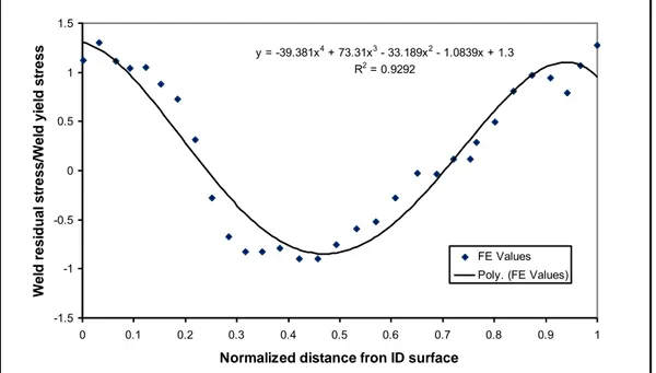
updated weld residual stress distributions,
updated repair schemes,
additional user defined input parameters, e.g., user defined weld residual stress distributions, user defined crack growth laws, user defined material data, user defined crack morphology parameters, and user defined random seed,
alternative crack initiation models, e.g., single versus multiple crack initiation analyses and arrival rate models,
alternative inspection and probability of detection (POD) routines,
allowing a variable stress distribution around the pipe circumference,
advanced probabilistic routines, e.g., discrete probability methods, including importance sampling, in addition to Monte Carlo simulation,
incorporating bootstrap methods for predicting confidence limits to provide insights into the variability of results, and
an updated graphical user interface (GUI) to reflect the most up-to-date changes to PRO-LOCA.
Section 2 of this report provides a detailed description of the technical basis for PRO-LOCA; both the probabilistic framework and the deterministic modules that make up PRO-LOCA. As part of this description of the technical basis for LOCA, the enhancements made to PRO-LOCA as part of MERIT are discussed in detail.
Section 3 of this report presents the results from the quality assurance (QA) checks that have been conducted as part of this program and the earlier NRC Large Break LOCA program. Modular QA checks have been conducted on most of the deterministic modules in PRO-LOCA to help ensure that the individual algorithms programmed into PRO-LOCA were programmed correctly. For example, results from the LBB.ENG2 through-wall crack stability module in PRO-LOCA were compared with results from the LBB.ENG2 J-estimation scheme in NRCPIPE, and exact agreement was found. Similar type comparisons were made for most of the deterministic modules in PRO-LOCA, e.g., surface and through-wall crack K-solutions, IGSCC and PWSCC initiation and growth modules, fatigue crack growth modules, surface crack stability modules, and leak rate module, and the agreement in those cases was excellent as well. A number of sensitivity analyses were also conducted. Those results are also presented in Section 3. A base case problem was solved and then individual input parameters were systematically changed to ascertain the effect of each of those input parameters on the resultant break probabilities. These analyses served two purposes. One, they helped identify coding errors in cases where the resultant changes in probabilities make little or no physical sense. Two, they helped identify the major risk factors in these types of probabilistic analyses by identifying which input parameters have the greatest effect on the predicted break probabilities.
Section 4 of this report discusses the results from these QA assessments and sensitivity analyses. Two parameters which seem to have a large effect on the LOCA probabilities are water chemistry for the BWRs and operating temperature of the PWRs. The operating temperature of the PWR was especially significant, where a 22 C (40 F) drop in temperature resulted in a 3 or 4 order magnitude decrease in the LOCA probabilities. Both of these parameters (water chemistry and temperature) effect both crack initiation and crack growth. Static bending stress, which also affects the crack initiation and growth characteristics, also had a significant effect on the LOCA probabilities. For the BWRs increasing the static bending stress from 20 MPa (3 ksi) to 50 MPa (7 ksi) resulted in a 1 ½ order of magnitude increase in the Category 2 LOCAs and a 3 order of magnitude increase in the Category 3 LOCAs. Similarly, doubling the static bending stress for the PWRs resulted in a 1 ½ order of magnitude increase in the Category 2 LOCAs and almost a 2 order of magnitude increase in the Category 3 LOCAs.
While inspection parameters had an effect on the LOCA probabilities, their impact did not seem to be as significant as those parameters which affect crack initiation and growth. Increasing the inspection interval from 10 to 20 years caused an order of magnitude or less increase in the LOCA probabilities. In a similar vein improving the quality of the POD curve caused a reduction in the LOCA probabilities although the impact was not that significant. To achieve a comparable order of magnitude decrease in LOCA probability required reducing the probability of detection by a factor of four. When a more realistic reduction in POD was assumed, the effect on the LOCA probabilities was relatively minor. A related parameter to inspection is leakage detection limit. The results for leakage detection limit are somewhat counter intuitive. For the analyses conducted as part of this effort, leakage detection limit does not seem to have that big of an effect on the resultant LOCA probabilities. This finding deserves further exploration.
In contrast to those parameters which affect crack initiation and crack growth, those parameters which affect crack stability did not seem to have as much of an effect on the LOCA probabilities. Neither material strength nor toughness had much of an affect on the LOCA probabilities. Even when the fracture toughness was decreased by a factor 20, the effect on the LOCA probabilities was relatively minor. Another parameter which would affect crack stability is an earthquake. The addition of an earthquake to the PWR load history resulted in about a one order of magnitude increase in the LOCA probabilities. While this seems significant it was shown that the magnitude of this earthquake was quite severe. With a more representative earthquake, the effect of the
earthquake would be expected to be less. The report concludes with a conclusion section in Section 5.
While PRO-LOCA represents a significant advancement in the technology, there is still work to be done. When PRO-LOCA was initially developed, the plan was to incorporate the latest state-of-art deterministic models into a probabilistic framework. Older deterministic methods such as limit load analyses for crack stability were replaced by the latest, most up to date methods such as J-estimate scheme routines based on elastic-plastic fracture mechanics principles. To facilitate and expedite this approach, the plan called for using legacy codes where available. As such, major sections of such legacy codes as SQUIRT, NRCPIPE and NRCPIPES were incorporated in their entirety into PRO-LOCA. While this sped up the developmental process, it did create a situation where a great deal of extraneous code was embedded within PRO-LOCA. This extraneous code has turned out to be somewhat problematic to the developmental process. Furthermore, some of the legacy variable definition has proved troublesome as the same parameter has a different variable name in different legacy codes. There have also been issues with some of the common block definitions. Finally, this legacy code was found to increase the run times for PRO-LOCA.
A further general limitation with PRO-LOCA is the level of quality assurance behind it. For example, as described in Section 3.1, a number of the deterministic modules in PRO-LOCA were subjected to some QA. However, the level of that QA and the overall QA for PRO-LOCA are not to the level required by ASME NQA-1. Part I of NQA-1-2008, Quality Assurance Requirements
for Nuclear Facility Applications, is organized as 18 separate requirements to mirror the
18-criteria structure of 10 CFR Part 50 Appendix B, Quality Assurance Criteria for Nuclear Power
Plants and Fuel Reprocessing Plants, and, as such is intended to meet and implement the
requirements of Appendix B. As a result of this lack of QA and the general lack of user experience, PRO-LOCA in its current state of development is considered to be a research code and any use of PRO-LOCA must factor that into consideration.
ACKNOWLEDGMENTS
The MERIT (Maximizing Enhancements in Risk Informed Technology) program was an international cooperative research program conducted at Battelle with assistance from staff at Engineering Mechanics Corporation of Columbus (Emc2). There were a total of six members in
this international group. The member countries and their respective Technical Advisory Group (TAG) representatives were:
Canada Mr. Michael Kozluk
Korea Dr. Young Choi
Sweden Dr. Bjorn Brickstad
United Kingdom Dr. Tracey Cool
United States
Electric Power Research Institute Mr. Paul Crooker
Nuclear Regulatory Commission Dr. Al Csontos
The authors would like to thank not only the MERIT TAG members, but also their numerous colleagues in their individual countries who made many valuable suggestions for improving PRO-LOCA.
1.0 INTRODUCTION
The MERIT (Maximizing Enhancements in Risk-Informed Technology) program is a 3 year multi-client international research program whose main objective was the further development of the PRO-LOCA probabilistic fracture mechanics (PFM) code. The membership in MERIT includes the US Nuclear Regulatory Commission (NRC), the Electric Power Research Institute (EPRI), SSM in Sweden, Rolls Royce in the United Kingdom, a consortium of interests in
Canada, and a consortium of interests in South Korea. The PRO-LOCA PFM code was originally developed for the US NRC as part of their re-evaluation of the emergency core cooling system (ECCS) requirements in 10 CFR 50.46. It was envisioned that PRO-LOCA would be used by the NRC on a periodic basis (i.e., every 10 years) as a tool to re-evaluate the break frequency versus break size curves which formed the technical basis for the transition break size (TBS) definition in the proposed rule change to 50.46, i.e., 10 CFR 50.46a. Other potential uses for PRO-LOCA include: (1) a general purpose PFM code for making leak-before-break (LBB), or extremely low probability of rupture (XLPR), assessments, (2) a flaw assessment tool for evaluating the failure probability of a piping system once a flaw is detected in service, and (3) a tool to help with the prioritization of maintenance activities, such as in-service inspections (ISI).
As part of the MERIT program a number of enhancements have been made to the PRO-LOCA code. Section 2 of this report provides a detailed description of the technical basis for LOCA; both the probabilistic framework and the deterministic modules that make up PRO-LOCA. As part of this description of the technical basis for PRO-LOCA, the enhancements made to PRO-LOCA as part of MERIT and the earlier NRC Large Break LOCA program are discussed. Section 3 of this report discusses the quality assurance (QA) checks and sensitivity analyses that have been conducted as part of this program and the earlier NRC program. Modular QA checks have been conducted on most all of the deterministic modules in PRO-LOCA to ensure that the individual algorithms programmed into PRO-LOCA were programmed correctly. For example, results from the LBB.ENG2 through-wall crack stability module in PRO-LOCA were compared with results from the LBB.ENG2 J-estimation scheme in NRCPIPE, and exact agreement was found. Similar type comparisons were made for most all of the deterministic modules in PRO-LOCA, e.g., surface and through-wall crack K-solutions, IGSCC and PWSCC initiation and growth modules, fatigue crack growth modules, surface crack stability modules, and the leak rate module, and the agreement in those cases was excellent as well. A number of sensitivity analyses were also conducted. As part of the main series of analyses, a base case problem was solved and then individual input parameters were systematically changed to ascertain the effect of each of those input parameters on the resultant LOCA probabilities. These analyses served two purposes. One, they helped identify coding errors in cases where the resultant changes in probabilities made little or no physical sense. Two, they helped identify the major risk factors in these types of probabilistic analyses by identifying which input parameters had the greatest effect on the predicted break probabilities. Section 4 of this report discusses the results from the QA assessments and the various sensitivity analyses conducted. Finally, the major conclusions reached regarding PRO-LOCA are discussed in Section 5.
In addition, there are two appendices to this report. Appendix A provides the details of the development of the geometric specific weld residual stress distributions included in PRO-LOCA. Appendix B is a brief description of the other major deliverables (other than PRO-LOCA, its GUI (graphical user interface) and its Users Manual) delivered as part of the MERIT program. These other deliverables include an updated SQUIRT leak rate code. SQUIRT was updated as part of this program to address a number of known issues with SQUIRT that had been identified with its increasing use. In addition, a new transition flow model to handle the flow regime between the single phase orifice flow regime and the two-phase flow regime governed by the Henry-Fauske model was developed and incorporated in SQUIRT. This transition flow model is discussed in
Section 2 of this report. Other deliverables from the MERIT program are an updated CIRCUMCK pipe fracture experiment database and a new leak rate experiment database.
2.0 DESCRIPTION OF PRO-LOCA CODE
This section of the report provides the technical basis for the PRO-LOCA code.
2.1 Probabilistic Framework
The user of the PRO-LOCA code has the option of a number of different probabilistic simulation schemes to chose from. In addition to the traditional Monte-Carlo simulation, the user of PRO-LOCA also has the option of using discrete probability methods, including importance sampling, when they want to predict very low probability events (on the order of 10-8 events).
2.1.1 Monte-Carlo Simulation
Monte-Carlo simulation (MCS) is a numerical scheme which solves a statistical problem by generating multiple deterministic scenarios of a model by repeatedly sampling values from the probability distributions for the uncertain variables and observing that fraction of the scenarios satisfying a relevant performance function or functions. The method is useful for obtaining numerical solutions to problems that are too complicated to solve analytically and can be used for any number of random parameters.
For the large break LOCA (LB-LOCA) problem, consider a generic n-dimensional random
vector,
1, , ,2
,T n
X X X
X which characterizes uncertainty in all system parameters, such
as geometry, material properties, inspection scheduling, load, initial flaws, etc. Figure 2.1 shows a schematic of the relationship between input vector
X
and the ith performance indicator (output) function gi(X
). The details of this output function are described in Section 2.13.Figure 2.1 Relationship between the input random vector X and the vector of output performance function gi(X)
To determine the occurrence probability of the ith performance indicator gi(
X
), the MCS method involves the following three steps: (1) generation of independent samples of the input random variables from their probability distributions, (2) calculation of a relevant performance function of the LOCA system, and (3) evaluation of the probability of occurrence of the performance function.2.1.1.1 Step 1 – Sampling Phase
Let 1, 2 , , N
x x x denote independent realizations (samples) of random input
X
, where N isthe sample size for MCS. For simplicity, consider the ith component Xi of input vector
X
with the cumulative probability distribution function,F x
Xi
i . Let Zi be a random variable uniformly distributed in the interval [0,1] and has the cumulative probability distribution function
i
Z i i
F z
z
. For a probability preserving transformation with the distribution functions of Xi and Zi being equal, the realization xi, of random variable Xi, can be obtained as
1
i
i X i
x F
z
(2.1)A two-step simulation technique can be developed based on this transformation. The steps are
A sample zi of Zi is generated, e.g., by using a standard random number generator available in any computer, and
A sample xi of Xi can be obtained from Equation 2.1. Thus, by generating independent samples of Zi, one can obtain from Equation 2.1 independent samples of Xi.
Hence, any random variable with any known distribution function can be easily generated using the transformation in Equation 2.1. For illustration purposes, transformation equations for random variables with normal and log-normal probability distributions are described below.
Normal Distribution: N ~ (i, i2)
PDF:
f
Xi
x
i
1
2
i
exp 0.5 (
x
i
i)
i
2
(2.2) Parameters: i = mean; i = standard deviationCDF: F xXi
i
x f x dxXi( )i i
(xi i) i
(2.3) is the CDF of standard normal random variableTransformation: 1( )
i i i i
x z (2.4)
Log-normal Distribution: LN ~ (i, i2)
PDF:
f
Xi
x
i
1
2
x
i i
exp 0.5 (ln
x
i
i)
i
2
(2.5) Parameters: i = mean; i = standard deviation; Vi = i/iCDF:
F x
Xi
i
xf x dx
Xi( )
i i
(ln
x
i
i)
i
(2.6)
2
2ln 1
;
ln
2
i
V
i i i i
is the CDF of standard normal random variable
Transformation: exp 1( )
i i i i
x z
(2.7)
In the original version of PRO-LOCA, external subroutines such as RNSET, RNGET, DRNUNF, DRNNOF, DRNWIB, and DSCAL from IMSL were used for random number generation. These routines have all been replaced by sampling procedures written at Battelle Memorial Institute so that a wider variety of distributions can be used and so that IMSL licenses are not an issue for any user.
A couple notes should be made about the sampling phase.
Sampling occurs:o At the beginning of each Monte-Carlo simulation, and
o At times during the plant history when a critical node is removed from service due to inspection or leak detection.
From the sampling, a timeline history of cracks initiated and loads on the critical node can be formed. The sampled variables include:o Material properties
Yield, tensile, Ramberg-Osgood, J-R curve, and
Fatigue and SCC growth exponents and coefficients
o Occurrence of transients
o Cracks and Detection
Fatigue and SCC time to initiations (and fatigue crack sizes), Pre-existing defects,
POD, and
Leak rate detection limit.
2.1.1.2 Step 2 –Repeat Evaluations
Following generation of input samples 1
,
2, ,
Nx
x
x
, letg g
i 1,
i 2, ,
g
i N denote thecorresponding samples of the ith performance function (output) gi(X) of the LB-LOCA system
that can be obtained from
j
( )j ; 1,2, ,i i
g g x j N (2.8)
Hence, all output samples of gi(X) can be obtained by conducting repeated deterministic
evaluation of the performance function gi(X), as schematically described in Figure2.1.
2.1.1.3 Step 3 – Determining Probabilities
Define Nf as the number of trials (analyses) that are associated with occurrence of the ith
performance indicator function. Then, the probability of occurrence of the performance indicator
Pi can be estimated by
Pr f ; 1,2, , i i N P g i m N X , (2.9)which approaches the exact value when N approaches infinity. In general, the minimum required number of trials (analyses) N must be at least
10
P
i for a 30-percent coefficient of variation of the estimator.2.1.2 Discrete Probability Distribution Method
Classically importance sampling methodologies have been employed in Monte Carlo simulations to assess low probability events. More recently adaptive methodologies for transformed density functions have been developed (Refs. 2.1, 2.2). Importance sampling methods for Monte Carlo become nearly intractable for complex engineering systems because it becomes increasingly difficult to remove the weighting function from the response sample. Adaptive methodologies provide fast, accurate answers for analytic functions. Unfortunately most engineering analysis does not employ analytic functions. In those cases, the standard practice is to employ response surfaces (Ref. 2.3) and analyze this approximation. The response surface will introduce a (usually) unquantifiable source of uncertainty unless one performs a Monte Carlo analysis to assess the uncertainty. In that case the adaptive methodology is useful if it is going to be employed for various distribution types and parameters.
A third option is the use of discrete probability distributions (DPDs). In this analysis, the input distribution, if it is analytically described, is discretized into a finite number of values, each value having an associated probability. If the number of discrete values is denoted as NBIN and there are
NV inputs to the analysis then to obtain the response DPD would require (NBIN)NV calculations.
For 100 discrete values and five input variables this would lead to 10,000,000,000 calculations. Clearly this would be no more efficient than the Monte Carlo analysis. However, if one treats the discrete space in the same manner as the continuous space one can employ a Monte Carlo
sampling of the discrete space to obtain an estimate of the response DPD. In fact, the same statistical analysis procedures used for polling can be used (Ref. 2.4). The distinct advantage that this method has over polling is that one knows, a priori, what the value of each discrete point is as well as its probability! The advantage of this procedure in engineering analysis is that the input DPD can be discretized so that the probability of the input value occurring is not made to be equal at each discrete point. For example, the first value and last values of the DPD can be set equal to the 1 in 10,000 value. The placement of the points in between these limits is set according to an optimization algorithm. By placing the lumped probability mass at the interval conditional mean points the error in using the discrete point will be canceled out from the expectation calculations.
One can illustrate the advantages and disadvantages of these methodologies by examining a theoretical example in which the response surface can be analytically calculated and comparisons of the DPD methodology to Monte Carlo and adaptive importance sampling analysis can be made. In this example it is demonstrated how events with probabilities of less than 1 in 1,000,000 can be estimated using 2,000 samples of the discrete space.
The goal of nearly any engineering system analysis is to calculate the response of a system to a variety of input values. One denotes the response of the system as R, the inputs to the analysis as the vector x, and the relationship between R and x as f. Then
R = f(x), x = (x1, x2, …, xN) (2.10)
The function f may be or may not be analytic. Thus f could represent a complex computer analysis, e.g. PROLOCA. The input vector x may have one, or more, components that are random variables. To begin one uses an overly simplified example to discuss the methods without becoming bogged down in the details of the engineering analysis.
The example selected is the addition of two random variables. Specifically
R = x1 + x2 (2.11)
If both of the inputs can be represented by a normal distribution with a mean value of k and a standard deviation of k for k equal to 1 and 2 then one can write down the mean and variance for R immediately.
R = 1 + 2 (2.12)
R2 = 1 2 + 22 (2.13)
In the classic Monte Carlo analysis one generates a random number, obtain the value of x1 by
inverting the normal distribution Cumulative Density Function (CDF), generate a second random number, obtain the value of x2 by inverting the normal distribution CDF, and add the two
numbers. This will generate a value for R that one denotes R1. One continues to do this many
times to generate a vector of responses denoted R = (R1, R2, …, RM). As M approaches infinity
the CDF for the response R will be approached. Of course if one is trying to calculate the extreme tails of the response distribution one will need, on the average, many, many samples. For the addition of two random variables this is not a very severe limit with today‘s computers so one will ignore this for the moment. It will become critical when one returns to realistic
An alternative method for generating the response CDF is to limit our calculations to points in the discrete space. In this case one defines a Discrete Probability Density (DPD) function for each of the inputs. Thus
)} , ( , ), , ( ), , {( 1,1 1,1 1,2 1,2 1, 1, 1 x p x p x NBIN p NBIN x (2.14) )} , ( , ), , ( ), , {( 2,1 2,1 2,2 2,2 2, 2, 2 x p x p x NBIN p NBIN x (2.15)
The response DPD is constructed by taking all possible combinations of the input DPDs. Thus R1 = (x1,1 + x2,1, p1,1*p2,1)
R2 = (x1,1 + x2,2, p1,1*p2,2)
. ..
RNBin = (x1,1 + x2,Nbin, p1,1*p2,Nbin)
RNBin+1 = (x1,2 + x2,1, p1,2*p2,1) (2.16)
RNBin+2 = (x1,2 + x2,1, p1,2*p2,2)
. . .
RNbin2 = (x1,Nbin + x2,Nbin, p1,Nbin*p2,Nbin)
One knows the resulting DPD is a Probability Density Function since
BIN BIN BIN BIN BIN
N I N I I N I N J J I N J I J J I
p
p
p
p
p
PdP
J
I
p
p
1 1 1 1 11
,
1
(2.17) are the two conditions which must be satisfied in order for a function to be a PDF. Let‘s begin byexamining a three point discretization of the normal distribution.
For a mean value of 10.0 and a standard deviation of 1.0 one knows that 33% of the probability lies between negative infinity and -0.42 (approximately). The next 33% lies between -0.42
and +0.42 (again approximately). The remaining 33% lies between +0.42 and plus infinity. But one must ask where should this probability mass actually be place. For the mean and
standard deviation assumed, the end points are (-∞, 9.58), (9.58, 10.42), and (10.42,∞).
Table 2.1 Three point DPD for N(,) = N(10,1)
xi pi
8.909 0.33334
10.000 0.33333
11.091 0.33334
If the probability mass is placed at these endpoints an artificial bias will be introduced into the response PDF. If one places the probability mass at the conditional mean of the interval then, on
the average, 50% of the time the value will be too large and 50% of the time the value will be too small, the error canceling out on the average.
Three Point Discrete Probability Distribution Comparison to Theoretical Values 0% 10% 20% 30% 40% 50% 60% 70% 80% 90% 100% 17 18 19 20 21 22 23 Magnitude CDF
3 point DPD NORMAL THEORY 3 point CDF
Figure 2.2 Three point DPD calculations 2.1.3 Importance Sampling in the Discrete Space
While the previous example is overly simplified to demonstrate the concept there is, theoretically, no upper limit to the number of bins that are used to define the individual DPD. Thus one could use 1,000,000 discrete intervals leading to 1,000,0002 or 1,000,000,000,000 points in a two
variable problem. In the case of N input variables and M bins there would be MN possible
responses. For a simple problem, in which there are less than 100 bins and only two variables the entire PDF of the response can be calculated. However, for more complex problems where there may be 10 variables and 100 bins describing the PDF one would have 1020 (10010) possible
outcomes. In this case one can use the identical strategy used in Monte Carlo analysis but instead of sampling from the continuous space one samples from the discrete space, i.e. from the 1020
values.
Because the number of values is finite (albeit a large finite number) one can use the same theory used to do census sampling to obtain the PDF of the response to as high an accuracy as desired. (see for example Reference 2.4).
Even more importantly one can change the way in which the individual DPD‘s for the input PDF is generated. Rather than using equal probability intervals one uses unequal probability intervals to perform importance sampling. The following section provides and example.
2.1.4 Sample Calculation of Importance Sampling Calculations
A simple example is the addition of two normal distributions. In this case we know that the response mean is equal to the sum of the two input mean values and the variance of the response is equal to the sum of the input variances. Thus the theoretical distribution of the response CDF can be calculated analytically and then compared with the DPD methodology output and the Monte Carlo output.
Figure 2.3 Comparison of the response CDF as calculated by Monte Carlo and RASCAL to theory
One adds two random variables with a mean of 10 and a standard deviation of 1.0. One can calculate the response CDF theoretically. One compares this theoretical prediction to
1. Monte Carlo analysis using 1,000,000,000 samples
2. RASCAL analysis using 50 bins of equal probability and 20 samples 3. RASCAL analysis using the first and last bin of 2.0 x 10⁻³.
Figure 2.3 shows the resulting calculations. Looking at the entire CDF does not give a very good picture and so one examines the tails of the distribution. In this case the CDF look very similar. Therefore, Figure 2.4 shows the tails of the distribution. In this figure one can see that the use of bin weighting for the DPD method allowed accurate estimates of the tails of the distribution using 1,000 less calculations.
Figure 2.4 Tails of the distribution for Monte Carlo and RASCAL analyses comparison to theory
2.1.5 Alternative Distributions
PROLOCA 2008 has been updated from the 2005 version by allowing the user to input additional distribution types. These distributions are described below and in Table 2.2.
The choice of distributions include:
Constant Uniform Normal Lognormal Weibull Exponential
Table 2.2 Description of distributions included in PRO-LOCA
Distribution PDF CDF Mean Variance
Uniform
a
b
x
f
1
)
(
b x a 0
)
(
x
f
a
x
or xb 0 ) (x Fa
x
a
b
a
x
x
F
)
(
a xb1
)
(
x
F
b x2
b
a
12 2 2 ba
Normal
2 2 22
1
)
(
xe
x
f
F
(
x
)
2
1
1
erf
x
2
Lognormal
2 2 2 ) ln(2
1
)
(
xe
x
x
f
F
(
x
)
1
2
2
1
erf
ln(
x
)
2
2 2
e
2
e
2
1
e
22
Weibull
xe
x
x
f
1)
(
x e x F( ) 1
1
1
2 21
2
21
1
Exponentialf
(
x
)
e
xF
(
x
)
1
e
x
1
21
2
Extreme Value Type II
x
e
xx
f
(
)
1
e
xx
F )
(
1
1
1 2 21
2
1
1
22.1.5.1 Uniform Distribution
Probability Density Function
a
b
x
f
1
)
(
axb 0 ) (x fx
a
or xbCumulative Distribution Function
0 ) (x F
x
a
a
b
a
x
x
F
)
(
axb1
)
(
x
F
xb Mean2
b
a
Median2
b
a
Variance
12
2 2
b
a
2.1.5.2 Normal DistributionProbability Density Function
2 2 22
1
)
(
xe
x
f
Cumulative Distribution Function
2
1
2
1
)
(
x
erf
x
F
Mean
Median
Variance 2
2.1.5.3 Lognormal DistributionProbability Density Function
2 2 2 ) ln(2
1
)
(
xe
x
x
f
Cumulative Distribution Function
2
)
ln(
2
1
2
1
)
(
x
erf
x
F
Mean 2 2
e Median
e
Variance
2
2 2
2 1
e
e
2.1.5.4 Weibull DistributionProbability Density Function
xe
x
x
f
1)
(
Cumulative Distribution Function
x e x F( ) 1 Mean
1
1
Median
ln(2)1 Variance
2 21
2
21
1
Since there is no analytic solution to invert the formulas for the and parameters one resorts to a Newton iteration method to calculate these values. Newton‘s method is:
x
x
f
x
f
x
x
n n n n 1(
(
)
)
One defines z as 1/ and write for f(z):
21
2
2 21
2)
(
1
z
l
z
l
z
f
f
One now notes the following derivative relationships:
(
z
)
(
z
)
z
z
)
(
)
(
z
z
z
where is the digamma function and is the gamma function. After much algebraic manipulation one finds
)
1
(
2
)
1
(
)
2
1
(
)
2
1
(
)
(
2 2z
z
z
z
z
z
f
) 1 ( 2 ) 1 ( ) 2 1 ( ) 2 1 ( 1 2 1 2 2 2 2 2 2 1 z z z z z l z l x xn n
The value of xn+1 provides a new estimate for 1/. One can then calculate from
1
1
All of these calculations assume that l is known. This is because one is only using two equations (for the mean and standard deviation) so only two unknowns, and , can be calculated.
2.1.5.5 Exponential Distribution
Probability Density Function x
e
x
f
(
)
Cumulative Distribution Function x
e
x
F
(
)
1
Mean
1
Median
ln(
2
)
Variance 2 21
2.1.5.6 Extreme Value Type II (Fréchet) Distribution
Probability Density Function
x
e
xx
f
(
)
1Cumulative Distribution Function
e
xx
F )
(
Mean
1
1
1 Median
1 ) 2 ln( 1 Variance 2 21
2
1
1
22.1.6 User Defined Random Seed
The random seed can be input as a fixed number by the user allowing the code to reproduce the same calculations or it can be randomly selected by the system clock. These routines are supplied in the INTEL compiler.
2.1.7 Random Variables In PRO-LOCA
Not every variable in PRO-LOCA is random. The variable selected to be treated as random variables are shown in Table 2.3.
Table 2.3 PROLOCA random variables
Number Parameter Mean Standard Dev Distribution
1 Yield Strength YIELDM YIELDS BYIELDDIST
2 Ultimate Strength UTSM UTSS BUTSDIST
3 Ramberg-Osgood exponent QNM QNS BNDIST
4 Ramberg-Osgood Coefficient FM FS BNDIST
5 JIc JIM JIS WJIDIST
6 m QMM QMS WMDIST
7 C ACONTM ACONTS WACONTDIST
8 User Fatigue C (FCGCOEF) AMEAN_F STDV_F IFCGDIST
9 (SCGCOEF) User SCC C AMEAN_S STDV_S ISCGDIST
10 Fatigue crack length FLAWMEANLEN FLAWSDLEN IFLAWDISTLEN
11 Fatigue crack depth FLAWMEANDEPTH FLAWSDDEPTH IFLAWDISTDEPTH
12 stress SIG0RS Weld residual SIG0RS_M SIG0RS_S ISIG0TYP
13 Weld residual stress XC XC_M XC_S IXCTYP
Crack morphology parameters
14 Global roughness GROUGH_M GROUGH_S ITYPGROUGH
15 Local roughness LROUGH_M LROUGH_S ITYPLROUGH
16 Global length GLFACT_M GLFACT_S ITYPGLFACT
17 Local length LLFACT_M LLFACT_S ITYPLLFACT
18 Number of turns NTL_M NTL_S ITYPNTL
19 SCLPAR WEIMEANTHETA WEISDTHETA IWEIDISTTHETA
20 WEISLP WEIMEANB WEISDB IWEIDISTB
21 Initiation time distributions
Weibull distribution SCLPAR WEISLP 4 (Weibull)
Non-Weibull distribution XTHETA XBETA ITIMEDIST
22 A182 YIELDMA182 YIELDSA182 WYIELDDIST
23 Leak Detection Leakdetm Leakdets 2 (Normal)
Each of the variables in Table 2.3 can be set to a deterministic value (constant ―distribution‖) or modeled as random via a uniform, normal, lognormal, Weibull, or extreme value distribution.
2.1.8 Parameters Hardwired into PRO-LOCA
In some cases the input parameters for PRO-LOCA can be user defined. In some cases they can be hardwired for the default models. In some cases they can be either. For instance, subunit size, crack length and crack depth are fixed in the default models, but can be input by the user in certain applications, depending on the needs of the problem and the desires of the user. Those parameters which are hardwired for the default models and their associated values are shown in Table 2.4.
Table 2.4 Hardwired parameters included in the default models of PRO-LOCA
Hardwired Parameter Value
Geometric model
Subunit size Percentage of pipe circumference based on 50 mm subunit length for 28-inch
diameter pipe
Time scale
Time scale 1 month
Material Properties
Material properties – option of using
library of default values Library of default material property values (means and standard deviations) of tensile and fracture toughness properties for both base metals and welds
Loads and Stresses
For transients; fully reversed loading R = -1
Weld residual stresses – option of using
default weld residual stress solutions Library of default weld residual stress solutions for 6 geometries; distribution function of distribution of yield strength
Pre-Existing Flaws
Number of flaws per inch of weld WinPRAISE (Ref. 2.10) equation
Flaw depths Statistical distribution of median crack depth, shape parameter, average crack depth,
and standard deviation on crack depth from Reference 2.9
Flaw lengths Distribution on aspect ratio (a/c)
Crack Initiation
Fatigue parameter KN KN = 2
Initiated fatigue crack length Lognormally distributed with medium value of 3 mm and standard deviation ln(b) =
0.85
Initiated fatigue crack depth (a) a = 3 mm
PWSCC initiated crack depth (a) a = 3 mm
PWSCC slope parameter (b) b = 3
Crack Growth
Fatigue threshold ΔKthres ΔKthres = 5 MPa-m1/2
PWSCC threshold Kthres Kthres = 9 MPa-m1/2
Crack Stability
Surface crack DPZP ―C‖ parameter C = 32
Through-wall crack DPZP ―C‖ parameter C = 18.3
Complex crack DPZP ―C‖ parameter C = 4.6
2.2 Geometric Model
In this version of PRO-LOCA, only one location or node is analyzed during each run. If the user requires the leak probabilities for the full system, individual runs for each location are required and the
probabilities must be summed to get the total probability. Typically, the worst location is used, and the failure probability is conservatively estimated by multiplying the worst-case node failure probability by the number of girth welds in the system.
In all cases, the user is allowed to choose what type of plant is to be analyzed. In the current version of PRO-LOCA, the user has four choices; PWR, BWR, BWR with hydrogen-water chemistry, and CANDU. This choice not only helps define the system to be analyzed but also sets the cracking mechanisms that will occur. In addition, the choice of hydrogen-water chemistry affects active, critical crack growth mechanisms.
The critical node analyzed is assumed to be one pipe diameter of specified size. The user is asked to input the location of the crack in the critical node. The options include base metal, manual arc welds, and inert gas welds. If a weld is chosen, it is assumed that the crack is either in the center of the girth weld or in the heat affected zone (HAZ)1.
In order to track the initiation and growth of defects through the plant life, the circumference of the critical node is broken into subunits. For the initial release of the code (June 2004 version), the subunit length was equal to approximately2 10 mm (0.4 inch). Each subunit was treated separately with a
predefined location around the circumference. It was also assumed that each subunit experienced an identical stress field, i.e., the stresses imparted on the pipe did not vary around the circumference. For the next released version of PRO-LOCA (December 2005 version), the subunit size was changed to
percentage of the pipe circumference. Sensitivity analyses suggested that the subunit size could be increased, thus decreasing the run time proportionately. Based on analysis of the Nine Mile Point IGSCC data, it was decided to fix the subunit length as a percentage of the pipe circumference. The final
percentage was established on the basis of a 50 mm (2.0 inch) subunit length for the 28-inch diameter Nine Mile Point recirculation system. In addition as part of the MERIT program, the assumption that each subunit undergoes an identical stress field was changed such that the stresses imparted on the pipe do vary around the pipe circumference. Furthermore, for the user defined arrival rate model for crack initiation that is incorporated into this latest version of PRO-LOCA, the number of subunits is not fixed, but instead is predicated on the number of initiated cracks predicted based on this arrival rate model.
2.3 Time Scale
In the PRO-LOCA code, one month time increments are assumed. The code is structured so that the user can input relevant node conditions, i.e., loads, transients, etc, either before the current plant year in operation, or after the year in operation. The data input before the year in operation is considered
deterministic, while the data input after is considered variable. The user can also input the year at the end of license and the year at the end of extended life.
2.4 Material Properties
For inputting material properties, the user is given two options. First they have the option of selecting the default properties from a library of materials. With this option the user will specify the material on each side of the weld. For similar metal welds, the two material selections will be the same, but for a
dissimilar metal weld, the user will specify different materials on each side. In the case of a dissimilar metal weld, the user will specify which material selection will govern the tensile properties. In addition to selecting the base materials, the user will also specify the weld type, e.g., Type 304 submerge-arc weld (SAW), Type 304 tungsten-inert-gas (TIG) weld, Inconel 182 weld, etc. A library of default material property values (both means and standard deviations) has been incorporated into the PRO-LOCA code. The library includes both tensile and fracture toughness properties. The default values were based on analysis of existing material property databases, most notably the PIFRAC database (Ref. 2.5) and the database of material property values developed by Argonne National Laboratories (Ref. 2.6). The list of materials, both base metals and weld metals, for which material property values are included in this library, is shown in Table 2.5. For most of these materials, tensile and fracture toughness properties were provided at multiple temperatures. For the cases where specific material data do not exist in the library, e.g., Type 304N or A508 Class II, generic sets of material property values for generic carbon steel, stainless steel, or cast stainless steel were developed and included in the PRO-LOCA library of material properties.
2Note that the number of subunits around the circumference had to be a whole number, so the actual length of a subunit may be
Table 2.5 List of materials included in material property library in the FY05 version of PRO-LOCA
Base Metals Weld Metals
Carbon Steels A106B A106B SAW
A106C A53 Grade A SAW
A53 Grade A A516 Grade 70 SAW
A333 Grade 6 A106C TIG
A155 STS 410 TIG
A516 Grade 70 Generic Carbon Steel Weld
A710 Grade A STS49 STS410 Generic Carbon Steel
Stainless Steel Type 304 Type 304 SAW
Type 316 Type 304 SAW (annealed)
Type 316L Type 304L SAW
Generic Stainless Steel Type 316 SAW
Type 304 TIG Generic Stainless Steel Weld Cast Stainless
Steel CF3A CF3 Generic Cast Stainless Steel Weld CF8M SAW
CF8 CF8A CF8M
Generic Cast Stainless Steel
Nickel Alloy Alloy 600 Alloy 182 Weld
Alloy 600 TIG
Generic Nickel Based Alloy Weld
For all of the material properties, statistical distributions were developed using the available material property test data. A database program was written to input additional data and analyze the data to extract the statistical parameters. For the PRO-LOCA code, all of the available data were used in developing the distributions. Specimen data were binned into 6 temperature categories (20-30C, 31-150C, 151-270C, 271-300C, 301-330C, and 331-350C). For materials and temperatures where less than five experiments existed, distributions were not generated. In these cases, either substitutions occur, or the code defaults to the generic material properties.
The database program written will allow additional data to be added as it is gathered or created. Therefore, as material property data is gathered from other programs, it can be added to the overall database. These database programs currently reside on the Emc2 server and can be accessed using the
following addresses:
http://www.emc-sq.com/Emc2MaterialDatabase/TensileTest.php - Tensile test database
http://www.emc-sq.com/Emc2MaterialDatabase/JRCurveSummary.php - Fracture toughness test database.
At this point, the database software is not integral with the PRO-LOCA code, so the material library embedded in PRO-LOCA will have to be manually changed if more data is added to the database.
For the second option, the user inputs their own material property values. For a chosen weld, the user will be asked to input mean values, with corresponding standard deviations, of the following material property values:
Base metal yield and ultimate strengths,
Weld metal yield and ultimate strengths,
Base metal elastic modulus,
Base metal Ramberg-Osgood coefficients (alpha and n), and
Weld metal fracture toughness coefficients (Ji, C, and m).
In addition, the user will also specify the distribution type for each of these material property values, i.e., constant, uniform, normal, lognormal, Weibull, exponential, or EV Type 1.
For fracture toughness, the J-R curve is specified by the power law relationship
mi
C
a
J
J
(2.18) where,J = Value of J at a given value of crack growth (Δa) Ji = Value of J at crack initiation
Δa = Amount of crack growth m = exponent
C = coefficient
These tensile and fracture toughness properties are used in order to make crack stability predictions. It should be noted that the user has the option of either using the default material property coefficients for subcritical crack growth hard wired into the code or providing their own material property coefficients for subcritical crack growth. These parameters will be fully explained in Section 2.8.
It is assumed that the material properties are time independent and contain no correction for strain rate. Thermal aging and dynamic strain aging effects are important in predicting crack behavior and may be included in a future release of this code.
2.5 Loads and Stresses
The loads and associated stresses used in PRO-LOCA are the static loads and stresses, including the weld residual stresses, plus the resultant stresses from both past and future transients.
2.5.1 Normal Operating Loads
The static normal operating load contributions are the result of pipe pressure, temperature, axial loads due to dead weight, static bending loads, plus the weld residual stresses. The axial stress component from the internal pressure (P) and the axial load (Fx) due to dead weight were calculated as: