Income inequality
and economic growth
BACHELOR THESIS WITHIN: Economics NUMBER OF CREDITS: 15
PROGRAMME OF STUDY: International
Economics
AUTHOR: Amanda Hult JÖNKÖPING December 2019
- An investigation of the OECD countries.
Bachelor Thesis in Economics
Title: Income inequality and economic growth.
Authors: Amanda Hult
Tutor: Michael Olsson
Date: 2019-12-09
Key terms: Inequality, economic growth, income distribution, OECD, Gini coefficient.
Abstract
Income inequality is in a majority of earlier studies more or less affirmatively agreed to be negatively related to economic growth. The underlying complexity of the connection lacks well-tried backing in the modern time. The main purpose of this research is to identify the relationship between income inequality and economic growth, but also the effects of other factors, such as human capital and investment. This is conducted with a panel data approach on 34 OECD countries with data over the period 1990-2010. Aggregate income inequality, represented by the Gini coefficient is used in the empirical estimation, together with two other variables to control for the income inequality at the bottom and top end of the income distribution. The results indicate the aggregate inequality level to be significantly and positively related to growth, while bottom end and top end inequality is seen to have a significant and negative relationship with growth. The level of GDP per capita, education and population growth is also seen to have an impact on economic growth.
Table of Contents
1. Introduction ... 1
2. Literature review ... 4
2.1 Theoretical literature ... 4
2.2 Empirical evidence ... 7
2.3 Methods and measurements ... 8
3. Data and method ... 10
3.1 Data sources ... 10
3.2 Description of variables ... 11
3.3 Descriptive statistics ... 12
3.4 Hypotheses ... 14
3.5 Empirical model ... 15
4. Result ... 16
5. Discussion ... 19
6. Conclusion ... 22
Reference list ... 24
1. Introduction
The average income inequality in the OECD countries has increased over the past decades and many of these countries are experiencing their highest inequality level ever (OECD Data, 2019). It has since 1985 increased and even if almost all of these countries have experienced an increasing level of inequality since then, the paths for different countries have varied. In the late 1970’s the increase notably started in United Kingdom, United states and Israel. About a decade later the increase was extensive throughout the OECD area. Over the 1990’s the income inequalities started to reach a historically high level in many earlier relatively equal countries. The overall increase has then continued up until today, aside from a decline between 2008 and 2010 (OECD Income Distribution Database, 2019). The average Gini coefficient in the OECD area has between the mid 1980’s and by the late 2000’s increased from 0.29 to 0.32. The rise has been high in both relatively equal countries like Sweden and Finland, but also more unequal ones like the US and Israel. However, the Gini coefficient has in a few countries not moved significantly, and in Greece and Turkey inequality has decreased. In the majority of the OECD countries, the top ten percent in the income distribution grew at a higher rate than the bottom ten percent, widening the income inequality gap. In 2011, the average ratio between the top ten percent and bottom ten percent of the income distribution was nine to one in the OECD countries. It however varied extensively across countries. It was relatively low in the Nordic and most of the continental European countries, ten to one in for example Italy and United Kingdom, around 14 to one in Turkey and the United states, while it reached a ratio of 27 to one in Mexico and Chile (Cingano, 2014).
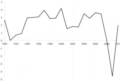
Economic growth, the increase in GDP over time is considered as a measure of effectivity and is per definition the increase in production of goods and services in a country over time. A sustained increase of growth is one of the fundamental prerequisite for a nation to maintain a high living standard and an economic security for its citizens (Nationalencyklopedin, 2019). In the OECD countries, the average growth in GDP per capita has between 1990 and 2010 been 2.12 percent with the highest average rate in Korea and Estonia, while lowest in Italy and Switzerland. We experienced a boom in the beginning of 1990’s after the German reunification, then it continued upwards but with a boom in the beginning of 2000’s as a result of the so called Dot-com bubble and another
boom related to the Great recession in 2007. This is observable in figure 1. Further, a graphical illustration of the evolution of the Gini index can be seen in figure 2. It is observable that the development of these factors follow a similar path, where also the Gini index answers to the economic shocks mentioned (OECD, 2019).
Figure 1. Average GDP per capita growth rate in the OECD countries between 1990 and 2010.
Figure 2. The average Gini index in the OECD countries between 1990 and 2010.
There are various theories about income inequality’s potential effects on economic growth. The main theories about positive effects are that income inequality is said to increase the incentive for people to work harder and that it will increase their savings and investments. In contrast, theories of the negative relationship stress that inequality will reduce savings as well as physical and human investment, and unbalance political and economical stability (Roth, 2018). That the results have been contradictory and not
robust, may be due to various approaches in different reports. Different choices of data quality, country coverage (development level), inequality indicators and estimation method have been seen to affect the outcome of the study (Cingano, 2014).
This study focuses on the OECD countries, on a twenty-year time period, starting in 1990. The accessibility of current and quality data has been a dilemma in empirical studies, and data on inequality and growth is available in the OECD area. This sample of relatively similar and highly developed countries, eliminates the risk of finding a correlation caused by the level of development. Further, less developed countries have been found to exhibit low quality data (Barro, 2000). The purpose is to investigate if there is a relationship between income distribution inequality and economic growth in the OECD countries, specifically between 1990 and 2010. The research questions can ultimately be defined as:
Does income inequality negatively affect economic growth in the OECD countries? What effect do the education and investment level have on economic growth? Depending on where in the income distribution inequality lies, is there a different effect on economic growth?
In chapter 2, the theoretical framework and empirical findings are presented, including what factors may have an effect on economic growth. It is concluded with appropriate methods and measurements. This is followed by a presentation of the data sources in chapter 3, along with the descriptive statistics and definitions of the variables. Following, the empirical model and correlation matrix are introduced. In chapter 4, regressions of the empirical model are presented and analysed. The results show a somewhat unexpected implication, that the Gini coefficient is positively related to economic growth, and top – and bottom end inequality have a negative relationship with growth. Education and investment show an expected positively relationship with growth. In chapter 5, reflections of the results are formed in the discussion. Conclusively, policy remedies are discussed and further studies are suggested.
2. Literature review
Inequality affects income growth by affecting different parts of its determinants, where some are fostering and others inhibitory. The main theories about a positive relationship between inequality and growth is the incentives to work harder and increase of savings and investment. Negative effects could be reduction of savings as well as physical and human investment, and unbalance in political and economical stability (Roth, 2018). In section 2.1 determinants of growth that in theory have been seen to be affected by inequality are presented, followed by how empirical studies support or reject these theories in section 2.2. Section 2.3 presents various methods and measurements used in earlier studies.
2.1 Theoretical literature
The classical economic theory finds inequality necessary for economic growth, where growth is driven by investments. According to this theory, people with higher income will save a higher percentage of their income than people with lower income. This will in turn increase investments and thereby growth. Inequality will hence favour everyone, since the contributory growth will make the poor better off compared to before (Roth, 2018). The neoclassical economic theory dominated the late ninetieth century. It assumes rational decision making based on the behaviour of the average individual, which contributed to a reduced focus on inequality issues. The neoclassic view was modified in the middle of the twentieth century, in conjunction with the construction of the Solow-model, when the technological development was found to be an important factor in the growth theory. In the 1980’s another growth theory arose, the endogenous growth theory, where the aspiration was for the growth determinants to be determined within the model. Human capital is here considered the driving force of growth (Nationalencyklopedin, 2019).
Galor and Maov (2004) identifies two fundamental approaches on how income distribution affects growth. The Classical approach and the Credit Market Imperfection approach. In the Classical approach, interpreted by for example Smith (1776), Keynes (1920) and Lewis (1954), saving rates are an increasing function of wealth which means inequality favors individuals whose marginal propensity to save is higher. In this way inequality boosts aggregate savings and capital accumulation which improves the
possibility of growth. As studies about the driving force of growth changed from being physical capital to human capital, the Credit Market Imperfection approach became more accurate. The relationship between inequality and growth is dependable on the credit market. An optimal credit market is one that is available to everybody, and lets human capital be allocated efficiently, however this is rarely the case. To invest in human capital often means to invest in an education, and with an unfair credit market, the ability for lower-income individuals will naturally be impaired. The Credit Market Imperfection approach however argues that equality in sufficiently wealthy economies reduces the negative effect of credit constraints on investment in human capital, which increases economic growth (Galor and Zeira, 1993). In line with the Credit Market Imperfection approach, Galor and Maov (2004) assumes human and physical capital to be fundamentally asymmetric, as human capital is embodied in individuals. In contrast to physical capital, the aggregate stock of human capital does due to physiological constraints subject its accumulation to diminishing returns. As the asymmetric assumption suggests, while human capital is positively affected by equality, inequality is favorable for physical accumulation, as long as the marginal propensity to save increases with income. In addition to education, health is considered as human capital and if low income individuals do not have the same possibilities to get high quality health care it will also affect their work opportunities which could increase the inequality even more (Roth, 2018).
The positive effect that incentives to work hard comes with greater inequality, is founded in the argument of individuals’ willingness to make more of an effort to achieve a higher rate of return. If there are great differences in income distribution, people has according to theory more to win by being productive. A higher productivity positively affects the technological development and economic growth is fostered. Similarly, a higher return to innovation and entrepreneurship will motivate people to put work into their ideas, hence invest in human capital (Acemoglu, Robinson and Verdier, 2015).
The fundamental macroeconomic balance, that savings is equal to investments, lays the ground for a country’s stable growth path. A restraint on consumption increases savings which makes an increase in production possible, and thereby development in growth. However, more profound conclusions can be made when analyzing the marginal savings
propensities at an individual level. The individual marginal consumption ratio and thereby savings ratio tendsto vary across groups in the income distribution (Todaro and Smith, 2011). Ray (1998) describes that an individual’s savings ratio is zero at an initial stage of increase in disposable income, up to a point around average income where it becomes positive and continues to rise with disposable income. At this point individuals’ propensity to save rise with the endeavor of a higher living standard. This aspiration and the propensity to save declines with a higher level of disposable income. Voitchovsky (2005) concludes that a higher level of inequality in the top end of income distribution promotes investment and thereby growth.
Population growth can also affect economic growth. Given a specific national income, a higher population growth rate means a lower income per capita. Hence, an increase in population growth will have a negative effect on growth rate in GDP per capita (Ray, 1998).
Inequality can affect economic stability by increasing people’s debts. The relative income hypothesis, formed by James Duesenberry, describes how income inequalities affect household debts. The position in income distribution will determine the household’s consumption level. By matching their consumption level with households nearby, a decrease in income will reduce their saving rate. Hence, greater income inequality leads to lower savings rates which can affect growth negatively (Roth, 2018).
Another argument for a negative relationship is that inequality will increase the demand of redistribution and higher taxes and thereby the political instability. According to the median voter theorem, politicians should follow the wishes of the median voter in order to maximize political support. If the majority of the population has a low or a middle income, the demand for redistribution will increase, and when the taxes on wages are high, the incentives to work will decrease and the growth will hence be negatively affected. The median voter theorem has later on been questioned with opposite claims. If the politics favour the rich, they may have the power to further influence it to their advantage, specifically with lower redistribution and taxes (Roth, 2018).
2.2 Empirical evidence
Over the past few decades the increased accessibility of comparable data has enabled investigating the topic on an aggregate level. Combined with the prominent role of the endogenous growth theory, the correlation between inequality and growth became an engaging topic again. Several studies since the 1990’s have taken advantage of this data, where some of them show a significant negative relationship between inequality and growth (Persson and Tabellini 1994), while other establish a negative relationship for poor countries but positive for rich countries (Barro, 2000). In the following section I will clarify if the presented theories have any support in empirical findings.
The theory of inequality’s positive effect on innovation and the incentives to work harder means that a highly unequal economy should have a higher level of innovation. The global innovation index is a widespread indicator on an economy’s level of innovation, that has been updated yearly since 2007. Studying the reports since then, there is no significant support of this theory. Relatively equal countries like the Nordics are often higher ranked than more unequal countries like the US (Global innovation index, 2019). The amount of patents a country has per capita can also give guidance of the innovation rate. If one studies patents per 1000 individuals in the OECD countries between 1996 and 2007, there is no evidence of a positive relationship between inequality and innovation level (Roth, 2018).
Researchers like Alesina and Rodrik (1994), Persson and Tabellini (1994) and Perotti (1996) all assume a relationship between inequality and investments in physical and human capital, and further between investments and economic growth. Lower investments in human capital is said to be a sequence of unfair credit markets. Hence, the connection between an economy’s level of human capital and the credit market’s availability needs to be studied. An economy’s educational level is often used as an indicator of the degree of its human capital. Finding a measurement of the credit market’s availability has however been a difficulty for researchers. Instead, researchers such as Persson and Tabellini (1994) and Perotti (1996) chose to directly investigate a relationship between inequality and human capital investments, by estimating a middle class income share as a measurement on equality. Nevertheless, the conclusion is a negative relationship, which means that inequality is in turn not found to foster economic
growth. From several studies Pickett and Wilkinson (2015) summarizes empirical results of mainly well developed countries, where the conclusion is that large differences in income distribution have had a negative effect on health and well-being. Madsen (2016) further establish poor health to inhibit individuals’ ability to work, which negatively affects economic growth. The causation of human capital and growth is however seen to go both ways. With higher income, people and governments can afford to spend more on education and health, and with greater health and education, higher productivity and incomes are possible.
It is argued that inequality will decrease the growth rate through political instability, by demanding higher taxes and redistribution. The findings of the correlation between greater inequality and higher taxes is divided. Perotti concludes that there is a negative relationship, that countries with higher inequality often also have lower tax policies (Perotti, 1996).The theory of a positive relationship is however supported empirically in newer studies, but is associated with countries with a low democracy level (Agnello et al. 2017).
The relationship between inequality and economic instability has been analysed empirically and the relative income hypothesis finds support in studies over countries like the US, Germany and the Netherlands. Bertrand and Morse (2016) shows that an increase in consumption among high income citizens leads to an increased consumption level also among low income citizens, even if there has been no change in their income level.
2.3 Methods and measurements
The discussed theories may have offsetting power and correlations are easily misleading when comparing countries as a whole. Many of the discussed negative effects are associated with inequality in lower income levels, while positive effects are often a sequence of the degree of inequality in the top end of the distribution (Voitchovsky, 2005). The distribution of income can be measured in different ways, but there are four criterions that needs to be fulfilled. (1) The anonymity principle, which states that it is irrelevant who earns the income. (2) The population principle, the absolute population size is irrelevant while proportions with different income levels of the population matters. (3) The relative income principle: relative incomes are relevant, not the absolute income
levels. (4) The Dalton principle: a regressive transfer – transfer from the “not richer” to the “not poorer” individual,will increase the inequality(Todaro and Smith, 2011). The most common used measurement is the Gini coefficient, which also fulfills all the criterions stated above. It covers a whole population and is easily compared between countries. It is an indicator of the level of income inequality and ranges from zero to one, where zero describes perfect equality, when the income distribution is perfectly equal and everybody has the same income. With a value of one, the Gini index describes a state of perfect inequality, which would be the case if all incomes would be allocated with only one person (or a group of people). There could be a problem with using only this measurement however. The theoretical positive and negative forces on growth with origin from inequality may be related to inequality in different ends of the income distribution. Many of the negative effects, such as political instability and lower investment seem to be related to inequality at the bottom tail of income distribution. In the same way, many of the positive effects seem to be an answer to the level of inequality in the top of the distribution. For example, a higher inequality in the top distribution will promote savings rates for higher income households (Voitchovsky, 2005). In this way, using only one statistic on inequality may be misleading depending on the differences of inequality in the top and bottom of the distribution. It will only show an aggregate result of its effects on growth, and a more complex result can be reached with additional indicators of inequality. Solutions in earlier studies have been to divide the income distribution into decile or quintile share ratios to test different parts of the distribution (Cingano, 2014).
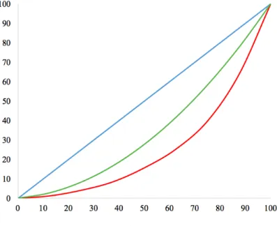
The Lorenz curve is a common tool when analyzing income distribution on an individual level. It is a graphical representation of the level of income inequality within an economy. The graph plots the cumulative percentage of recipients on the horizontal axis. That means that at point ten, the poorest ten percent of the population are accounted for, and at point 50 the poorest half are presented. Continuing up to point 100 where the total population has been accounted for. On the vertical axis the cumulative percentage of income is plotted. Perfect equality is symbolized by a diagonal line from origin to the upper right corner. At every point at that line, the percentage of income received is equal to the percentage of income recipients. For example, at point 30.30, 30 percent of the total income is distributed to 30 percent of the population. In contrast to the equality line, the Lorenz curve represents the actual relationship between the percentage of recipients and
the percentage of income. Perfect inequality would be represented by a Lorenz curve following the horizontal axis and the right vertical axis up to the upper right corner. In reality, the Lorenz curve lies somewhere below the equality line, where a greater gap indicates a greater inequality. The Gini coefficient can be calculated by calculating the ratio of the area between the equality line and the Lorenz curve, over the total area below the equality line. To get it in a percentage form, this value is calculated with 100. A graphical demonstration of the Lorenz curve can be seen in figure 1 below, where the red line represents a relatively higher level of inequality than the green Lorenz curve. The blue line is the equality line (Todaro and Smith, 2011).
Figure 3. The Lorenz curve.
3. Data and method
Panel data is used in this analysis, for the time period 1990 to 2010. The sample consists of 34 OECD countries. In the following section I introduce the dataset used, a description of the included variables, the descriptive statistics, a correlation matrix, hypotheses of the expected outcome and lastly the empirical model.
3.1 Data sources
Over the recent decades the accessibility, especially in more industrialized countries, has widened thanks to projects of data collection for comparability. World Income Inequality
Database (WIID) is one of those and also where statistics of the Gini coefficient was collected. Data of education level was collected from Barro-Lee Dataset, while the other variables were gathered from The World Bank. Data for education level was only available on a five-year basis, why a linear interpolation was used to estimate values for omitted years.
3.2 Description of variables
The independent variables will be indicators of the Gini index, GDP per capita, human capital, population growth and investments and is further described below. All these variables will be lagged five years to consider the amount of time it takes for the variables to affect growth. The model is in line with the one used by Li and Zou (1998), but with two added variables, representing population growth and investments, used in other similar studies. Further, by suggestion of Voitchovsky (2005), inequality in different parts of the income distribution will be controlled for by adding two variables representing inequality in the top and bottom end of the distribution. Two models will hence be estimated, where the first one includes variables for bottom - and top end inequality, and the second one excludes them. Technological progress is a theoretical determinant in GDP growth, but is generally excluded when estimating inequality’s effect on growth (Perotti, 1996; Forbes, 2000). A simplified empirical model helps to maximize the degrees of freedom, which reduces the risk of a misleading result (Cingano, 2014).
Y
Economic growth is estimated by growth in GDP per capita. The dependent variable, Y, is the average yearly growth rate on a five-year basis, in real PPP adjusted GDP per capita in each OECD country.
GINI
As a description of the aggregate income inequality in each country, GINIrepresents the Gini coefficient. The variable is analyzed in its percentage form, by being multiplied by 100, which means that a value of zero implies perfect equality, while a value of 100 implies perfect inequality.
BOT, TOP
According to Voitchovsky’s (2005) suggestion, an extended measure of inequality is included. BOT and TOP, which respectively represents the level of inequality in the bottom and top end of the income distribution, is included in model 1. Income distribution is divided in quintiles and quintile ratio Q3/Q1 is considered when analyzing inequality at the bottom end of income distribution, and Q5/Q3 at the top end. In this way the ratio between the quintiles on each side of the median is exploited and risk of mismeasurement is minimized (Voitchovsky, 2005).
GDP
GDP represents the PPP adjusted GDP per capita in each country. Countries with initially lower GDP per capita tends to experience a relatively faster growth rate.
EDUC
Investment in capital and especially human capital is an important factor of determining the economic growth in the endogenous theory. EDUC represents the average years of education in the population aged 25 and over, where three levels of education are included, primary, secondary and tertiary. A higher rate of education is expected to foster economic growth in a country.
POP
POPreflects the yearly percentage population growth. Population growth has been seen to reduce a country’s economic per capita growth.
INVEST
The fundamental macroeconomic balance, that savings is equal to investments, lays the ground for a country’s stable growth path. A restraint on consumption increases savings which makes an increase in production possible, and thereby an increase in growth. INVEST represents the gross fixed capital formation as a percentage of GDP.
3.3 Descriptive statistics
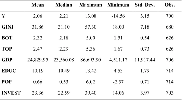
The descriptive statistics are presented in table 1. Number of observations varies between 626 and 714 for different variables, where data of inequality for the top and bottom end
of distribution was scarcer than for any other variable. Short panel data is analyzed, which means that the number of cross-sectional subjects, 34 countries, is greater than the number of time periods, which is 16 because of the five-year period adjustment.
Table 1. Descriptive statistics.
Mean Median Maximum Minimum Std. Dev. Obs.
Y 2.06 2.21 13.08 -14.56 3.15 700 GINI 31.86 31.10 57.30 18.00 7.18 680 BOT 2.32 2.18 5.00 1.51 0.54 626 TOP 2.47 2.29 5.36 1.67 0.73 626 GDP 24,829.95 23,560.08 86,693.90 4,511.17 11,917.44 706 EDUC 10.19 10.49 13.42 4.53 1.79 714 POP 0.66 0.53 6.02 -2.57 0.71 714 INVEST 23.36 22.59 39.40 14.06 3.97 703
The descriptive statistics show a few extreme maximum and minimum values. While the mean of GDP growth is 2.06, the maximum value is 13.08 and was estimated in Estonia 1997, and the minimum value, -14.56, was also from Estonia but in 2019. The maximum Gini coefficient (57.30) was estimated in Chile in 1999 and the minimum value (18) was estimated in Slovakia 1990 and 1991. The GDP per capita level also ranges relatively widely, with a maximum value of 86,693.90 in Luxembourg in 2008, and a minimum value of 4,511.17 in Chile 1990. The minimum value of education level (4.53) was estimated in Turkey 1990. The maximum value of investment level (39.4) was estimated in Korea 1991.
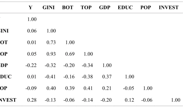
Table 2 presents the correlation matrix, where the values show a value between zero and one, where zero indicates no correlation between the variables, while one indicates a perfect positive relationship and minus one indicates a perfect negative relationship (Gujarati, 2003).
Table 2. Correlation matrix.
Y GINI BOT TOP GDP EDUC POP INVEST
Y 1.00 GINI 0.06 1.00 BOT 0.01 0.73 1.00 TOP 0.05 0.93 0.69 1.00 GDP -0.22 -0.32 -0.20 -0.34 1.00 EDUC 0.01 -0.41 -0.16 -0.38 0.37 1.00 POP -0.09 0.40 0.39 0.41 0.21 -0.05 1.00 INVEST 0.28 -0.13 -0.06 -0.14 -0.20 0.12 -0.06 1.00
The variables in table 2 exhibit a mainly positive relationship between each other. Reasonably, BOT and TOP are strongly positively related to GINI with values of 0.73 and 0.93respectively, which could be a result of sharing a common trend. This implies multicollinearity between GINI and TOP. Also BOT and TOP are strongly positively related. I will for this reason analyze an additional model where TOP but also BOT are excluded (Gujarati, 2003). This is done with low risk of specification errors, since theory does not require these variables to be included for the estimation of economic growth. There are cases of negative correlation, with the most negative values between GDP and GINI 0.32), TOP and GDP 0.34), EDUC and TOP 0.38) and EDUC and GINI (-0.41).
3.4 Hypotheses
Based on the theoretical review, hypotheses of the variables’ effect on economic growth are stated as follows.
H1: Aggregate inequality has a negative effect on the GDP growth rate.
H2: Inequality in the bottom end of income distribution has a negative effect on the GDP
H3: Inequality in the top end of income distribution has a positive effect on the GDP
growth rate.
H4: GDP per capita has a negative effect on the GDP growth rate.
H5: Education level has a positive effect on the GDP growth rate.
H6: Population growth has a negative effect on the GDP growth rate.
H7: Investment level has a positive effect on the GDP growth rate.
3.5 Empirical model
The empirical model will try to capture how economic growth is affected by income inequality. Countries with higher inequality in a top quintile will according to theory be united with a higher level of innovation, while countries where the greatest inequality lies in the bottom end of the distribution, perhaps have issues like economic and political instability (Cingano, 2014). The empirical model will be constructed similarly to the ones Alesina and Rodrik (1994) as well as Li and Zou (1998) analyzed.
Y" = 𝛽&+ 𝛽(𝐺𝐼𝑁𝐼",-./+ 𝛽0𝐵𝑂𝑇",-./+ 𝛽4𝑇𝑂𝑃",-./+ 𝛽6𝐺𝐷𝑃",-./+ 𝛽/𝐸𝐷𝑈𝐶",-./
+ 𝛽;𝑃𝑂𝑃",-./+ 𝛽<𝐼𝑁𝑉𝐸𝑆𝑇",-./+ 𝜀
(1)
Model 2 excludes BOT and TOP and will hence be:
Y" = 𝛽&+ 𝛽(𝐺𝐼𝑁𝐼",-./+ 𝛽0𝐺𝐷𝑃",-./+ 𝛽4𝐸𝐷𝑈𝐶",-./+ 𝛽6𝑃𝑂𝑃",-./+ 𝛽/𝐼𝑁𝑉𝐸𝑆𝑇",-./+ 𝜀 ",-(2)
Referring back to the hypotheses, each hypothesis is respectively verified if β1<0, β2<0, β3>0, β4<0, β5>0, β6<0 and β7>0.
4. Result
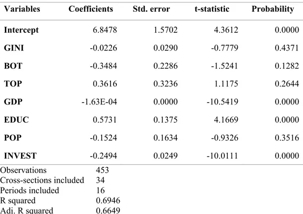
Hausman test and Chow test were first conducted, which indicated that the fixed effect model was appropriate for the regression model. Table 3 presents the results of model 1, in which BOT and TOP are included.
Table 3. Fixed effect regression model – results of model 1.
Variables Coefficients Std. error t-statistic Probability
Intercept 6.8478 1.5702 4.3612 0.0000 GINI -0.0226 0.0290 -0.7779 0.4371 BOT -0.3484 0.2286 -1.5241 0.1282 TOP 0.3616 0.3236 1.1175 0.2644 GDP -1.63E-04 0.0000 -10.5419 0.0000 EDUC 0.5731 0.1375 4.1669 0.0000 POP -0.1524 0.1634 -0.9326 0.3516 INVEST -0.2494 0.0249 -10.0111 0.0000 Observations 453 Cross-sections included 34 Periods included 16 R squared 0.6946 Adj. R squared 0.6649
At a first glance of the results, it is evident that every variable except from INVEST have the expected direction of impact on growth. The variables explain a relatively high variation of economic growth, specifically 69.46 percent. However, not all variables exhibit a significant correlation with growth. The inequality indicators together with POP show an insignificant relationship with growth. GDP per capita significantly affect GDP growth and as expected, is negatively related to GDP growth. All else equal, for every one unit increase in GDP per capita, the 5-year average GDP growth rate decreases with 0.000163. A country’s education level is as expected positively related to economic growth. All else equal, for every one unit increase in education level, growth increases with 0.5731 units. Further, GDP growth decreases with 0.1524 for every one unit increase in population growth. The noteworthy thing in these results is the negative relationship between investments and growth. The relationship is expected to be positive, but
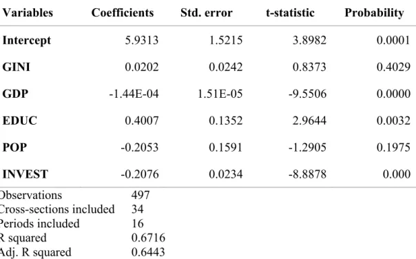
investments does according to table 3 reduce economic growth with 0.2494 units for every one unit increase in investments. The results of model 2, where BOT and TOP are excluded, are presented in table 4.
Table 4. Fixed effect regression model – results of model 2.
Variables Coefficients Std. error t-statistic Probability
Intercept 5.9313 1.5215 3.8982 0.0001 GINI 0.0202 0.0242 0.8373 0.4029 GDP -1.44E-04 1.51E-05 -9.5506 0.0000 EDUC 0.4007 0.1352 2.9644 0.0032 POP -0.2053 0.1591 -1.2905 0.1975 INVEST -0.2076 0.0234 -8.8878 0.000 Observations 497 Cross-sections included 34 Periods included 16 R squared 0.6716 Adj. R squared 0.6443
The variation of Y described by the independent variables is lower than in model 1, yet still relatively high, specifically 67.16 percent. As in model 1, all variables except from GINI and POP have a significant relationship with economic growth. Overall, the results look similar to those presented in table 3.
The Durbin-Watson test was conducted for model 1 and 2, which resulted in values of 0.5250 and 0.4790 respectively. Hence, there are signs of positive autocorrelation. An essential assumption for a linear regression model is homoscedasticity, that the variance of the disturbance terms is the same. To check for heteroscedasticity, the Breusch-Pagan test was conducted. With a significance level of five percent, the p-value of 0.0000 indicates heteroscedasticity. A possible source of heteroscedasticity is skewness in one or several regressors included in the model. In a normally distributed model, the skewness should be zero and the kurtosis should be three (Todaro and Smith, 2011). The observed skewness is -0.52 and the kurtosis is 5.08, and skewness could indeed be the source of
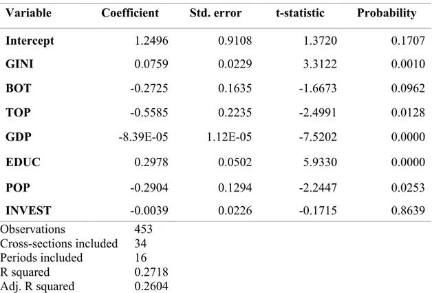
heteroscedasticity. To resolve for heteroscedasticity, White’s robust regression is run and the results are presented in table 5 below.
Table 5. White’s robust standard error regression - results of model 1.
Variable Coefficient Std. error t-statistic Probability
Intercept 1.2496 0.9108 1.3720 0.1707 GINI 0.0759 0.0229 3.3122 0.0010 BOT -0.2725 0.1635 -1.6673 0.0962 TOP -0.5585 0.2235 -2.4991 0.0128 GDP -8.39E-05 1.12E-05 -7.5202 0.0000 EDUC 0.2978 0.0502 5.9330 0.0000 POP -0.2904 0.1294 -2.2447 0.0253 INVEST -0.0039 0.0226 -0.1715 0.8639 Observations 453 Cross-sections included 34 Periods included 16 R squared 0.2718 Adj. R squared 0.2604
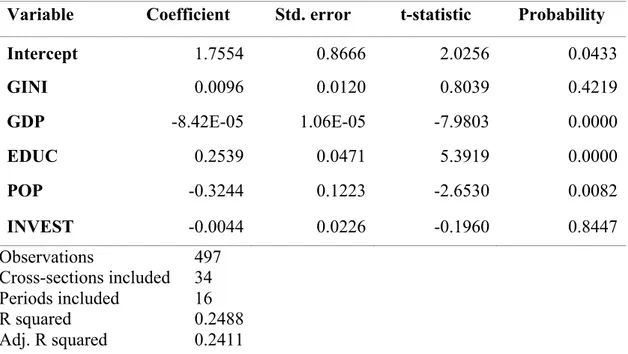
Now, the standard errors are assumed to be correct and at a ten percent significance level, all variables except from the intercept and INVEST are significant. GINI, BOT, TOP and POP are now significant, in contrast to the results from the fixed effect model. According to these results, a one unit increase in aggregate level of inequality, economic growth increases with 0.0759. The coefficient for the variable TOP is -0.5585, which means that a one unit increase in the top distribution inequality, decreases economic growth with 0.5585, all else equal. The change in economic growth due to a one unit increase in EDUC is lower according to these results, specifically 0.2978. Hence, all else equal, a one unit increase in years of education would lead to an increase of 0.2978 in GDP per capita growth. The decrease due to an increase in POP is here lower, -0.2904 in GDP growth for every one unit increase in population growth, all else equal. However, the variation of the dependent variable is only explained by 27.18 percent of the independent variables. The White’s robust regression model was also conducted for model 2 and the results can be seen in table 6.
Table 6. White’s robust standard error regression - results of model 2.
Variable Coefficient Std. error t-statistic Probability
Intercept 1.7554 0.8666 2.0256 0.0433 GINI 0.0096 0.0120 0.8039 0.4219 GDP -8.42E-05 1.06E-05 -7.9803 0.0000 EDUC 0.2539 0.0471 5.3919 0.0000 POP -0.3244 0.1223 -2.6530 0.0082 INVEST -0.0044 0.0226 -0.1960 0.8447 Observations 497 Cross-sections included 34 Periods included 16 R squared 0.2488 Adj. R squared 0.2411
In accordance with model 1, INVEST has in model 2 still an insignificant relationship with economic growth. Also GINI shows an insignificant result. Otherwise, the magnitude of the independent variables’ effect on the dependent variable is very similar to the results in table 5.
5. Discussion
To establish a reliable result there are several factors to take into consideration. The availability of high-quality data has over the decades increased and is not considered a problem in this analysis. Furthermore, the inclusion of countries needs to have a similar level of development. The Human Development Index is used to reveal a country’s development level, and is a “summary measure of average achievement in key dimensions of human development” (UNDP, 2019).With the majority of the OECD countries with a HDI index above 0.8, the sample seems reliable in that aspect. The construction of the empirical model and estimation method are also essential for a reliable result. Some version of the Generalized Method of Moments (GMM) regression estimator is the most common method in similar studies, which exploits the largest source of variation in inequality across countries, while also accounting for country-specific explanatory factors. It has also been common to use a lagged dependent variable, when the GMM
method is convenient because of correlation issues that may arise consequently. An unlagged dependent variable was used here which did not require the application of such an advanced estimation method.
When the empirical model is constructed, autocorrelation, heteroscedasticity and multicollinearity are circumstances that need to be accounted for. Autocorrelation and heteroscedasticity are dealt with by applying White’s robust standard error regression model. Multicollinearity is present in model 1 but since BOT and TOP was removed in model 2, it is not considered a problem. However, the results from the two models are equivalent. Considering the process to the final results from White’s robust regression, these results are assumed to be the most reliable and those are also the ones considered in the following section. However, the goodness of fit of the model seems weak, considering that the explanation of the economic growth is only explained by 27.18 and 24.88 percent respectively. Model 1 is reasonably higher, since R2 always increases when variables are added. The adjusted R2, which is a modified version of R2 that accounts for the number of determinants of the model was 0.2604 and 0.2411 for model 1 and 2 respectively. Hence the somewhat higher value of model 1 implies that the added variables BOT and TOP actually improves the model more than would be expected by chance.
In section 3, a negative relationship between aggregate inequality and economic growth was hypothesized. However, the results indicate the opposite relationship, which contradict theory and many earlier studies’ conclusions. The results of aggregate income inequality’s effect on economic growth however confirm several earlier findings, like for example Li and Zou (1998) who studied panel data with the fixed effect model and the random effect model, with a similar empirical model to what was used in this study. Based on panel data, also Forbes (2000) and Barro (2000) established a positive relationship in high and middle-income countries, which most of the OECD counties are considered to be. Earlier studies with regressions based on cross-sectional data tend to yield negative coefficients when estimated with the Ordinary Least Squares. Forbes (2000) explains this negative or significant bias to be a consequence of the country-specific, time-invariant and non observable variables estimated. On the contrary, empirical reports using panel data tend to yield a positive or insignificant relationship, because of its ability to eliminate data variation and aggravating measurement error biases Cingano (2014). Voitchovsky
(2005) exhibits an insignificant result of the aggregate inequality. In this case the result was indeed significantly positive.
What needs to be considered is that the Gini coefficient reflects the overall inequality within a country. A disadvantage of the Gini coefficient is the possible misleading results, since it reflects the aggregate level of inequality and fails to specify where in the income distribution the inequality lies and in this way allows to conceal the underlying complexity of the relationship. Considering the positive result, one could think that the top inequality had a higher influence on aggregate inequality. The negative effects on growth is in theory associated with bottom end income inequality, while the top end income inequality is associated with positive effect on growth. In the results however, both BOT and TOP are seen to have a significantly (at a ten percent significance level) negative relationship with GDP growth. The direction of the correlation between TOP and economic growth is contradictory to theoryand to what Voitchovsky (2005) found. However, there is not much empirical evidence on how inequality in different parts of the income distribution effects economic growth.
The so called catching-up effect is a theory that assumes that poorer economies grow faster by being able to take advantage and replicate richer economies’ production methods and technologies. In this way they are catching up richer countries and sometimes even converge in terms of income per capita. There are however sometimes limitations in form of lack of capital. If analyzing the used data, this is confirmed when the countries with an initial GDP per capita below 10,000 has an average growth rate of 3.51 percent, while economies with an initial GDP per capita above 15,000 had an average growth rate of 1.68 percent. The majority of the studied countries have an initial relatively high GDP level and as in line with theory and empirical finding, the results show that an increase in GDP per capita seems to negatively affect GDP growth, if even only slightly.
The identified positive relationship between education level and economic growth confirms theory. A higher level of educated citizens opens possibilities for development in production methods. The quality of education can however have an impact and is not considered in this study. This is associated with the social mobility which can be constrained with a restricted credit market. A restricted credit market prevents talented individuals from low-income households to invest in an education and social mobility is
hence hindered. Where education is not available for everyone, talent is wasted and the production effectivity may be jeopardized. Even with subsidized educations, income inequality may increase the differences of the quality between regions (Roth, 2018). The empirical model is in ways simplified with for example technological progress disregarded as an explanatory factor, as it is generally not used in models estimating the effect of inequality on growth (Perotti, 1996; Forbes, 2000). However, technological development is associated with the increase in economic growth related to the incentives to work harder that comes with income inequality. High income inequality and possibility to higher return to innovation gives people more to win by being productive and invest in human capital, which positively affects the technological development and hence economic growth. In this way a part of the technological development is accounted for in the variable EDUC (Acemoglu, Robinson and Verdier, 2015).
All else equal, as the population increases in an area, the total GDP is distributed between a higher number of people, and logically the GDP per capita decreases. This is also reflected in the results.
In conclusion, hypothesis one and three is according to the results rejected, that is, it can be rejected that the Gini coefficient affects economic growth negatively. It can also be rejected that inequality in the top end of income distribution has a positive effect on economic growth. Hypothesis two and four to six is not rejected. Hence, it cannot be rejected that inequality in the bottom end of income distribution has a negative effect on economic growth. Furthermore, it cannot be rejected that GDP per capita level or population growth have a negative effect on economic growth. Not either that educational level has a positive relationship with growth. Since there is no significant relationship between INVEST and economic growth, hypothesis seven is also rejected.
6. Conclusion
The results of income inequality’s effect on economic growth is contradictory in this study, since GINI is positively related to growth, while both BOT and TOP have a negative relationship with growth. It makes theoretical sense that bottom end income
inequality affects growth negatively. To make sure it does not increase, government transfers to low-income households are essential for preventing them of falling further back in the income distribution. Also increasing the access to public services, like high-quality education and health care are important when aspiring the lower-income households not to fall back in the income distribution. Such policy remedies both reduces income inequality immediately but also by fostering social mobility in the long run. Income inequality in the top of income distribution could be regulated with some type of tax policy (Cingano, 2014).
As inequality can affect growth through different economic factors, theoretical studies discuss how it is relevant to adjust for time lags in order to visualize the amount of time it takes to materialize for different mechanisms. In the attempt to control for this, a time lag of five years was created for every variable which finds support in many newer studies, like for example Li and Zou (1998) and Voitchovsky (2005). However, different factors reasonably affect growth after a different amount of time, which is not considered in these models. Perhaps changes in variables such as population growth and GDP have a more direct effect on economic growth, while changes in education level and investment takes longer to have an impact on economic growth. This is suggested for further studies to take into account. Further, more ratios of bottom – and top end inequality could be tested, for a more thoroughly estimation. Other empirical models and estimations methods could be considered and combined, since most approaches face some kind of drawback or inconvenience that may affect the result. Another measurement for human capital, where health is included may be considered for a more reliable result. This study was limited to the OECD countries over a twenty-one-year period. Earlier studies have included a broader number of counties and for longer time periods. What is critical when studying growth fluctuations over a relatively long period of time can for example be change in social structure and economic shocks. Dummy variables for these kinds of factors are considered in some of earlier studies, but could perhaps improve the result of a study of this size as well.
Reference list
Acemoglu, D., Robinson, J. A. and Verdier, T. (2015). Asymmetric Growth and Institutions in an Interdependent World. Working paper.
Agnello, L., Castro, V., Tovar Jalles, J. and Sousa, R. (2017). Income Inequality, Fiscal Stimuli and Political (In)Stability. International Tax Public Finance, 24: 484-511.
Alesina, A. and Rodrik, D. (1994). Distributive Politics and Economic Growth. The Quarterly Journal of Economics, 109 (2): 465-490
Barro, Robert and Jong-Wha Lee. (2013). "A New Data Set of Educational Attainment in the World, 1950-2010." Journal of Development Economics, 104: 184-198.
Barro, R.J. (2000). Inequality and growth in a panel of countries. Journal of Economic Growth, 5 (1): 26-29.
Bertrand, M. and Morse, A. (2016). Trickle-Down Consumption. Review of Economics and Statistics, 98 (5): 863–879.
Cingano, F. (2014). Trends in Income Inequality and its Impact on Economic Growth. OECD Social, Employment and Migration Working Papers, No. 163, OECD Publishing. Pp. 9-54.
Galor, O. and O. Moav. (2004). From Physical to Human Capital Accumulation: Inequality and the Process of Development. Review of Economic Studies, 71 (4): 1001– 1026.
Galor, O. and Zeira, J. (1993). Income Distribution and Macroeconomics. Review of Economic Studies, 60 (2): 35–52.
Global Innovation Index. (2019). Retrieved September 24, 2019, from https://www.globalinnovationindex.org/Home
Gujurati, D. (2003). Basic Econometrics. 4th edition. Boston: McGraw-Hill. Pp. 320-351. Li, H. and H. F. Zou. (1998). ”Income Inequality is not Harmful for Growth: Theory and Evidence.” Review of Development Economics, 2 (3): 318–334.
Madsen, J. B. (2016). Health, Human Capital Formation and Knowledge Production: Two Centuries of International Evidence. Macroeconomic Dynamics, 20 (4): 909–953.
Nationalencyklopedin, tillväxtteori. (2019). Retrieved September 11, 2019, from:
http://www.ne.se/uppslagsverk/encyklopedi/lång/tillväxtteori
OECD (2011). Divided we stand: Why inequality keeps rising, OECD Publishing. (https://www.oecd.org/els/soc/49499779.pdf)
OECD (2019). Gross Domestic Product. Retrieved September 23, 2019, from https://data.oecd.org/gdp/gross-domestic-product-gdp.htm
OECD. (2019). Income Distribution Database (IDD). Retrieved September 23, 2019, from https://data.oecd.org/inequality/income-inequality.htm
OECD. (2019). Income Inequality. Retrieved September 23, 2019, from https://www.oecd.org/social/income-distribution-database.htm
Partridge, M. (1997). ”Is Inequality Harmful for Growth? Comment.” The American Economic Review, 87 (4): 1019–1032.
Perotti, R. (1996). Growth, Income Distribution, and Democracy: What the Data Say. Journal of Economic Growth, 1 (2): 149-183.
Persson, T. and Tabellini, G. (1994). Is Inequality Harmful for Growth? American Economic Review. Pp. 600-621.
Pickett, K. E. and Wilkinson, R. G. (2015). Income Inequality and Health: A causal review. Social Science & Medicine, 128: 316–326.
Ray, D. (1998). Development Economics. 1st Edition. Princeton: Princeton University Press.
Roth, P. (2018). Landsorganisationen i Sverige. Jämlikhet och Tillväxt. Pp. 6-21.
Todaro, M. P. and Smith, S. C. (2011). Economic Development. 11th Edition. Pp. 109-249. Boston: Pearson Addison-Wesley.
The World Bank. (2019). Retrieved September 23, 2019, from: https://data.worldbank.org/
UNDP. (2019). Human Development Reports. Retrieved November 30, 2019, from: http://hdr.undp.org/en/content/human-development-index-hdi
UNU-WIDER, World Income Inequality Database (WIID4), (2018). Retrieved September 23, 2019, from:
http://www.wider.unu.edu/
Voitchovsky, S. (2005). “Does the profile of income inequality matter for economic growth?” Journal of Economic Growth, 10 (3): 273–296.