The Grid of Sweden

(1)

Degree Project in Criminology Malmö University

90-120 credits Two-year master Faculty of Health and Society

A MICRO-UNIT ANALYSIS OF VULNERABLE

NEIGHBORHOODS

MIA PUUR

(2)

THE GRID OF SWEDEN

A MICRO-UNIT ANALYSIS OF VULNERABLE

NEIGHBORHOODS

MIA PUUR

Puur, M. The Grid of Sweden. A Micro-unit Analysis of Vulnerable Neighborhoods. Degree project in criminology 15 Credits. Malmö University: Faculty of Health and Society, Department of Criminology, 2020.

Through a national collection, the Swedish Police identify and classify vulnerable neighborhoods. Areas are assessed through police perceptions regarding high concentrations of certain problems and criminal activity, such as public acts of violence with risk of harming third parties, open drug markets and organised crime structures. The purpose of this study has been to see whether it is possible to statistically discover these neighborhoods based on socioeconomic and demographic data. Initially, in a national comparison, areas that are defined as vulnerable neighborhoods by the national collection, was compared with other areas in the country. This was done based on a statistical grid consisting of squares with the dimension of 250 x 250 meters, with each square holding information about socio-demographic data. The main aim has been to identify a statistical model that more objectively can identify squares that are vulnerable or not, compared to the police's more subjective assessment. Result from logistic regression analyses implies that vulnerable neighborhoods from the national collection show greater odds at having high concentrations of residents with foreign background, higher unemployment rates and more households with single parents. Lastly, the best fitted regression model for explaining these areas by the means of pseudo R2-value, were used to calculate a prediction value for each square. This value was then analysed using a GIS-software, to discover any areas that in the national collection was classified as vulnerable, but according to the model no longer met the criteria, and then vice versa. The overall result indicate that it is possible to discover areas with higher concentrations of certain characteristics seen in vulnerable neighborhoods, using spatial analyses and logistic regressions of micro-places, to more objectively classify these areas. By aggregating crime data, the result of this study can in the future mean a more effective implementation for police authorities.

Keywords: crime, geography, micro-places, police authorities, spatial analysis,

(3)

ACKNOWLEDGEMENTS

I would like to begin by thanking Manne Gerell, my supervisor, who gave me the opportunity to write this paper and therefore made this study possible. With quick responses and helpful suggestions, I thank you for your encouragement and support throughout this whole process.

I want to express a special gratitude to my family, partner and our three beautiful children for hanging in there by my side and supporting me all the way.

(4)

CONTENT

ACKNOWLEDGEMENTS ... 3

CONTENT ... 4

INTRODUCTION ... 5

Aim and research questions ... 5

BACKGROUND ... 6

Theoretical frameworks ... 6

Social disorganisation theory and collective efficacy ... 6

Broken windows ... 7

Strain ... 7

The labelling perspective ... 8

Previous research ... 8

Fear of crime and organised crime ... 9

The national collection ... 9

METHOD ... 10 Units of analysis ... 10 Ethical reflections ... 11 Data ... 11 Material ... 12 Variables ... 13 Considerations ... 14 Analytical strategy ... 14 RESULT ... 14 Characteristics ... 14

A statistical model in progress ... 15

Using a vulnerable prediction estimate ... 17

Category A ... 18

Category B ... 18

Category C ... 19

Category D ... 20

DISCUSSION ... 20

The modifiable areal unit problem ... 21

Study limitations ... 22

CONCLUSION ... 23

REFERENCES ... 24

(5)

INTRODUCTION

Structural societal changes have created many challenges in contemporary Sweden, where social exclusion and marginalisation are a growing issue in and around many urban areas of the country (Sjöberg & Turunen 2018). Low socioeconomic status and living segregation is a common reality for a relatively extensive group of individuals who has not been integrated in the overall society (ibid.). The National Council of Crime Prevention in Sweden sometimes refer to areas or neighborhoods where these structures are common as socially vulnerable (NCCP 2015) and these areas also tend to show higher levels of criminal activity which have an impact on the local community with signs of, among other things, feelings of unsafety (NCCP 2018). The Swedish Police also describe these neighborhoods as vulnerable and they are nowadays seen as a growing societal issue (Police 2017; Police 2019). The Swedish Police further divide these neighborhoods into geographical units and classifies them as vulnerable-, at risk- or particularly vulnerable neighborhoods and they mostly occur in bigger urban areas, but also in smaller cities of Sweden (NCCP 2016).

Levels of fear of crime in socially vulnerable areas are significantly higher than in other urban areas and the causes are related to visible disorder and criminal behaviour that affect residents, regardless of whether they are exposed to the crime itself or not (NCCP 2018). Both social and physical disorders, such as littering, car fires and vandalism are known to have a negative impact on residents’ feelings of safety, along with nuisance from groups of young people, joyriding and open drug sales (ibid.). In a British context, Brunton-Smith and Sturgis (2011) found similar patterns where fear of crime was influenced by visible signs of low-level disorder and weak social, economic and structural characteristics. Another phenomenon, that got a lot of media attention in Sweden the last few years and which have been found to have a major impact on resident’s feelings of fear, are shootings (NCCP 2018). The above issues can be associated with criminal gangs or groups of young boys and men, who’s behavior is perceived as threatening (ibid.). Often these problems are clustered, and tend to occur on specific courtyards, streets or squares, rather than in entire residential neighborhoods (ibid.).

The Swedish police has since 2015 published three reports regarding vulnerable neighborhoods in which they identify areas that can be classified as vulnerable through a national collection (Police 2019). Every local police district has to fill in a document for each neighborhood they perceive have a few problems, with the purpose to create a unified view of the area in order to classify areas that can be regarded as vulnerable (ibid.). All the areas are assessed through police perceptions regarding public acts of violence that risk harming third parties, open drug markets, resident’s tendency to participate in legal processes, the police ability to carry out their mission, any parallel social structures, local organised crime groups and extremism (ibid.).

Aim and research questions

The purpose of this study is to investigate whether it is possible to statistically identify vulnerable neighborhoods based on socioeconomic and demographic data. The Swedish police evaluate vulnerable areas through police perceptions regarding high concentrations of certain problems and criminal activity, such as public acts of violence with risk of harming third parties, open drug markets and organised

(6)

criminal structures. The aim of this study therefore is to see if it is possible to create a statistical model that more objectively can classify vulnerable neighborhoods, which further could mean easier implementation for police authorities.

The current study is national where places that are defined as vulnerable neighborhoods by the Swedish police national collection, are compared with other places in the country. Based on a statistical grid consisting of squares with the dimension of 250 x 250 meters, socio-demographic data will be analysed in order to see if whether it can be understood why certain squares are considered to be included in a geographical context where problems are believed to exist. The main aim is therefore to identify a statistical model that more objectively can identify squares that are vulnerable or not, compared to the police's more subjective assessment. The study intends to answer the following four questions:

1. What are the characteristics of squares that coincide, in whole or in part, with vulnerable neighborhoods that are reported in the national collection?

2. How can we statistically, through socio-demographic data, identify vulnerable neighborhoods from the national collection? 3. Are there neighborhoods which, statistically, appear to be vulnerable, based on question 2, but which are not classified as such?

4. Are there neighborhoods which, statistically, do not appear as a vulnerable neighborhood, based on question 2, but which are still classified as such?

BACKGROUND

Given the term vulnerable neighborhood has no recognised international definition, the upcoming background and previous research focuses on literature regarding neighborhoods or areas where poverty and crime are believed to affect the local community. The context of place is emphasized throughout the background and in the end of this section, the national collection is described more in detail.

Theoretical frameworks

Below, four theoretical frameworks are briefly explored with the aim to explain why crime tends to be more concentrated in certain places or areas. Social

disorganisation theory is described with a primary focus on how residents’ ability

to practice social control in their neighborhood, either fosters criminal behaviour or diminishes it. Also, in the light of social disorganisation, Broken windows will also be mentioned; a perspective where social and physical disorder have a negative impact on criminal behaviour. For a more critical approach, strain theory and the

labelling perspective will also be described within a structural context. Social disorganisation theory and collective efficacy

The social disorganisation theory aims to explain criminal behaviour through neighbourhoods’ local social and economic conditions (Anselin et al. 2008) and is based on the understanding that crime clusters in certain areas but not in others and that areas known as disorganised neighbourhoods suffer from lower levels of informal social control - something that plays a crucial part in generating

(7)

environments more favourable to crime. The theory was initiated from Park and Burgess ecological model which aimed to explain structural variations in urban neighborhoods and later Shaw and McKay described how poverty, residential instability, population heterogeneity and family disruption are factors which influence criminal behaviour in a geographical context (Sampson 2006). Crime rates were therefore more influenced by the context of the neighborhoods rather than by the residents. According to Sampson and colleagues (1997) these neighborhoods lack what they call collective efficacy, which means that residents show little trust in one and another and an unwillingness to interfere for the common good of the neighborhood. Therefore, these neighborhoods have little social cohesion which also are shown by signs of neglect, for example physical disorder such as litter and trash, vacant and abandoned buildings, and graffiti (Anselin et al. 2008). The theory of collective efficacy states that when collective efficacy is low, it is unlikely that residents would intervene in a neighborhood where the rules are unclear and where the residents suspect or fear each other (Sampson 2006).

Broken windows

The idea of Broken windows arose from the belief that crime is not caused by “bad” individuals, but rather “bad” areas. The basis of the theory is that crime thrives in areas where less serious disruptions of order are allowed to freely occur and where local actors fail to fix the problems (Wilson & Kelling 1982). The main statement of the perspective is that a broken window, which goes unrepaired, leads to other windows around also gets broken (ibid.). According to the theory, social order disturbances from unpredictable people, as well as physical disorder can lead to serious crime which further leads to a gradual decay of residential areas (ibid.). Neighborhoods with growing social and physical disruptions tend to create insecurity, which among residents affects informal social controls in the local community (ibid.).

Strain

Merton's theory of strain explains how social structures exert a certain pressure on some individuals in society to engage in various types of behavior, including criminal conduct (Merton 1938). Life goals are culturally defined in society and are shared through common societal values, but opportunities for achieving these goals can be very diverse and among others depending on where you come from or where you live (ibid.). The discrepancy between the goals set by society and individuals’ tools or opportunities to achieve them can lead to some individuals seeking alternative, and every so often deviant, methods (ibid.). Strain therefore increases the risk of deviant behaviour for individuals who are less favoured through the balance between life goals and the tools to achieve them. The problem in society, according to the theory, is that social structures limits the starting points to reach goals and become successful in a legitimate way; and individuals from lower socio-economic backgrounds find it more difficult since they are already "behind" from the beginning and therefore needs to be exceptionally talented or just lucky in order to achieve the goal set by society (Lilly et al. 2011). Agnew (2001) notes that there are four types of distinguishing factors that are likely to lead to strain. These are if the strain is perceived unfair, if the feeling of strain is perceived extensive, if strain occur in connection with low social control, or if strain creates pressure or incitement to participate in criminal acts (ibid.).

(8)

The labelling perspective

This approach originated from Howard Becker, who in 1963 pointed out that crime or deviance is a result of society’s reaction to certain individuals or incidents of crime (Sundberg & Puur 2020). Different members of society are at different risk of being perceived as deviant by others, and this perception is essential in explaining deviant and criminal behavior (ibid.). It has also been suggested that juveniles from certain socioeconomic groups are at higher risk of being publicly labelled (Farrington 1977) and that juveniles fitting the description of coming from socially and economically deprived areas are more likely to be detected due to higher police presence in these neighborhoods (Sampson 1986). Likewise, McAra and McVie (2012) find in their study that juveniles are being labelled, not because of their own deviant behaviour, but rather by reputations based on their family’s socioeconomic conditions and by living in socially deprived areas (Sundberg & Puur 2020). The reason for labelling individuals living in socially vulnerable neighborhoods can be quite complex. As Sampson and Raudenbush (2004) argue, cultural stereotyping indicates that individuals hold persistent belief’s regarding disadvantaged minority groups to certain social images, including those of crime, violence and disorder (Sundberg & Puur 2020). In their study they find that the social structure is a more powerful predictor of perceived disorder, rather than observed disorder; and therefore, they suggest that cultural stereotypes about disorder are as prominent as objective signs of disorder (ibid.).

Previous research

Formal and informal social controls are affected, among others things, by low socioeconomic status, high residential mobility and ethnic heterogeneity; which do not occur in a void and thus are rooted in structural contexts and the society’s overall political and economic climate (Bruinsma et al. 2013; Sampson et al. 1997). Areas characterized by disadvantaged social and economic conditions are considered insufficient to control and monitor deviating behavior in areas (Sutherland et al. 2013) and therefore may explain why neighborhoods vary in their ability to achieve common goals and public order (Sampson et al. 1997). Places with much social and physical disorder are more likely to be characterised with higher criminal activity (Telep & Weisburd 2018), and as described above, the geography of crime have been linked to the inability of the social place to control antisocial and deviant behaviour. Furthermore, it has been found that high socioeconomic status is a protective factor as higher crime levels occur to a lesser extent in places where the population is wealthier and have the opportunity to practice more effective informal social control (Telep & Weisburd 2018).

Literature with a focus on criminology in urban environments has for a long time maintained that the criminal distribution in society can be related to the type of land use different areas uphold (Ceccato 2012; Wuschke & Kinney 2018). It is quite understandable that crime appears different in a place where there is only residential housing compared to a place where there are only commercial actors or especially a place with industrial premises (Ceccato 2012). The risk of crime at a specific place thus varies depending on the built environment and its characteristics, but also depending on the human activities that the site generates during a specific time (Ceccato, 2012; Davies & Bowers 2018; Wuschke & Kinney 2018).

(9)

Fear of crime and organised crime

Reports, from the Swedish Council of Crime Prevention, show that residents in socially vulnerable areas experience higher feelings of fear of crime compared to residents in other urban areas and much of the feelings of unsafety can be linked to visible disorder and crime (NCCP 2018). Some types of criminal acts signal stronger feelings of unsafety than others and individuals can be affected both indirectly, through feelings of insecurity and concern about being exposed to crime, or directly through threats of violence by criminal groups (ibid.). In general, feelings of fear of crime has been found to be higher in residential areas that are characterised by high unemployment, low income levels and multi-family homes (NCCP 2009).

The physical and social context of a residential area also affects local organised crime and how criminal groups are able to operate (Crocker et al. 2018). Occasionally it is discussed how organised crime has nested into the local community and their methods tend to reflect the characteristics of the residential area itself (ibid.). Criminal gangs are formed in areas which are characterised by high crime, concentrated poverty, high population density and single-parent households (Valasik & Tita 2018). In Sweden there have been an increase the recent years regarding shootings and explosions and where the increase is linked to criminal networks and vulnerable areas (Sturup et al. 2019). Shootings are about five times more likely to occur in socially vulnerable areas and the escalation is limited to these locations with a similar pattern for detonated hand grenades (ibid.). The increased firearm violence in Sweden mostly affects younger men (Sturup et al, 2018) and the increase in lethal firearm violence can often be linked to criminal conflicts (NCCP 2019).

The national collection

According to the Swedish Police definition, a vulnerable neighborhood is characterised by low socioeconomic status where criminals have an impact on the local community and where the situation is considered serious (Police, 2019). The influence of crime is more linked to the social context of the area than to the actual intent of the criminals to take power and control over the local community (ibid.). The impact of crime in vulnerable neighborhoods can be direct pressure, for example through threats or extortion, or more indirect, such as public acts of violence that risk harming third parties, open drug markets or an obvious frustration with society (ibid.). The effect of criminal activity in vulnerable neighborhoods is that residents experience feelings of unsafety, which in turn leads to a reduced tendency to report crimes and to participate in any legal processes (ibid.).

A particularly vulnerable neighborhood is characterised by a general reluctance to

participate in the legal processes and there may also be systematic threats and acts of violence against witnesses, informers, or injured parties (Police, 2019). The situation in the area makes it difficult, or almost impossible, for the police to carry out their mission, which have led to regular adaptation of working methods (ibid.). A particularly vulnerable area also includes, to a certain extent, parallel societal structures and extremism, such as systematic violations of religious freedom or strong fundamentalist influence that limits people's freedoms and rights (ibid.). Some residents from these neighborhoods have also travelled to participate in combat in conflict areas (ibid.)

(10)

The police have also identified an in-between level called a risk neighbourhood, which is an area that meets all the criteria for a vulnerable neighborhood but does not really reach the criteria that characterise a particularly vulnerable neighborhood (Police 2019). However, the situation is so alarming that there is an imminent risk that the area reaches the upper level unless adequate measures are taken (ibid.). Another aggravating feature is if there are other vulnerable neighborhoods in close proximity to a particular vulnerable neighborhood; then there is a risk of collaboration between criminal individuals or networks in these areas and the situation therefore must be considered serious (ibid.).

In the report from 2019 there were 60 neighborhoods in Sweden that were classified; 22 neighborhoods were graded as particularly vulnerable, 10 neighbourhoods as being at risk and 28 neighborhoods were graded as vulnerable neighbourhoods (Police 2019).

METHOD

This paper has a quantitative approach with a focus on the geography of crime and structural variations which will be assessed through spatial analysis. Geographical information systems, GIS, has enabled criminological researchers to dynamically link maps providing visual representations of the relationship between two or more characteristics, such as for example poverty rates and crime rates (Anselin et al. 2008). Geocoding allows scholars to detect areas containing clustered characteristics, for example crime hot spots or underlying criminogenic features, which is done by transforming addresses into precise geographic coordinates (ibid.). However, geocoding is not enough to be sure that what we see is statistically significant clustering’s; in order to do so, more formal methods must be employed and therefore, the data in the current study will also be analysed further through independent t-tests and logistic regressions.

Units of analysis

The choice of which type of spatial units to use when conducting spatial analysis is something that must be done with consideration (Rengert & Lockwood 2009) and the area size and boundaries is typically solved pragmatically (Oberwittler & Wikström 2009). Studies usually depend on official data regarding the socio-demographic and physical make-up of neighborhoods, which are normally available only for pre-defined administrative units such as blocks, block groups or tracts (ibid.) Census tracts is a commonly used unit due to that they often are the most convenient units to get hold on, though there are some issues around aggregations that is connected to these types of politically or administration bounded units (Rengert & Lockwood 2009). Therefore, scholars of crime and place often argues that the unit of analysis in relation to crime should be narrowed to smaller geographical units, for example only as big as buildings, addresses, cluster of addresses, or street segments (Oberwittler & Wikström 2009).

A street block is a small unit of analysis and are often used in studies of crime and place and can be defined as the four blocks faces on a square street block (Kim, 2018). A theoretical weakness of blocks is that it assumes that individuals socially interact with others on the street behind them and not with those who live across, but on the same street (ibid.). Street segment or face blocks, as it sometimes are

(11)

referred to in the literature, is another type of small unit of analysis that also has been repeatedly used and are defined as both sides of a street between two intersections (Weisburd et al, 2004). These small units of analysis can be referred to as micro-places and are defined as specific locations within a larger social environment of a community or neighborhood (Kim 2018).

It is important to test underlying relationships between structural characteristics and crime at micro-places due to that the characteristics of place may both affect consistency or change in criminal activity (Kim 2018). The units of analysis in this study therefore consists of a grid of squares with the dimension of 250 meters x 250 meters of all of Sweden’s urban areas. This grid contains socioeconomic and demographic data where data from the Police containing their national collection of vulnerable neighbourhoods have been aggregated to each square that coincide whole, or in part with a vulnerable neighbourhood. The total number of squares with the size of 250 x 250 meters are 113 551 in the whole of Sweden. Researchers also argue that it is beneficial to examine whether structural characteristics in micro-places are similar compared to other micro-places within proximity (see for example Kim 2018). To address this, the current paper also examines how many of the squares within a diameter of 275 meters respectively 625 meters from the centre of each square that also shows the same structural characteristics.

Ethical reflections

When conducting any scientific research or study, it is important to consider and reflect about ethics in order to ensure that research is done with a responsible approach (Vetenskapsrådet 2017). Further are these reflections and considerations important for the quality of research and implementation of the results that are utilized to improve our society (ibid.). When performing research, it is crucial that the researcher consider the potential benefits of the study to the possibility of harm (Maxfield & Babbie 2015). Nevertheless, the current study is not examining individuals nor sensitive data and are therefore not obligated to reflect further about volunteerism, integrity, confidentiality and anonymity - aspects that are usually very important when studying populations. Even though the units of the current study are small, there are no data that can be drawn down to specific individuals. Still, when categorising or dividing some areas as vulnerable, criminogenic or deprived, it is valuable to at least consider how the label can affect and stigmatise local communities and their residents. Urban inequality is a factor in contemporary Sweden, but nonetheless should one not forget the potential harm of labelling vulnerable neighborhoods, something that has been considered during the work with the current paper.

Data

The socioeconomic and demographic data used in the current study was collected by the Central Bureau of Statistics (SCB) in Sweden and most of the data is from 2019 and some from 2017. Data from the national collection regarding the vulnerable neighborhoods has been collected by the Swedish police authorities in 2019. The socioeconomic and demographic data consists of four groups of features within the population of each square: Swedish or foreign background, household

types, employment, and age.

The last few years many individuals have immigrated to Sweden and by the end of 2019, 19.6 percent of the Swedish population were foreign-born (SCB 2020). The data on Swedish or foreign background contains five attributes, or variables, collected 2019: born residents with two born parents; domestic-born residents with one domestic-domestic-born parent and one domestic-born parent;

(12)

foreign-born residents; domestic-foreign-born residents with two foreign-foreign-born parents; and the total number of residents. People have immigrated to Sweden for various reasons and for different periods of time and therefore there are many discrepancies between foreign born residents from different countries of birth in terms of age, gender and why one has immigrated (SCB 2020). One can have come as refugee or in need of protection, as student or for labour, or one can have been adopted or be a relative of any person living in Sweden (ibid.).

The data regarding households in Sweden are based on a register where a household consists of individuals listed in the same residence and are divided in three main types; living together (people living together as married, in registered partnership or in a cohabitation relationship), single households and other households (all other households where at least one person in the home does not have close relationships with anyone else in the household, neither a child nor a parent, nor has a couple relationship with someone else in the household) (SCB 2019). Examples of other households are households with three-generation housing, residents’ friends or colleagues (ibid.). In the current dataset from 2019, these households’ types are further divided into six attributes: living together with children; living together without children; single households with children; single households without children; other households; and the total number of households.

The two employment attributes from 2019 contain number of residents that are employed and number of residents between the ages of 20 to 64; which is the working age in Sweden. Last the attributes of age consists of eight pre-defined age categories from 2017: age 0 to 6; age 7 to 15; age 16 to 19; age 20 to 24; age 25 to 44; age 45 to 64; age 65 and up; plus the total number of residents.

Data regarding vulnerable neighborhoods have been received from the Swedish Police and the data about municipalities was received from SCB and showing population, municipality code, municipality name, urban name, and county name.

Material

The data received from SCB came in the form of five shapefiles with each data shown as a layer with associated attributes (variables). All the socio-demographic attributes have subsequently been joined together in one layer so that each square is connected to all four different attributes. Though, not all data, or layers, involve the same number of squares; some have more squares, and some has less squares and this is probably due to that where squares are missing, there most likely are too few residents to show a specific attribute. The attribute with most squares were Swedish and foreign background, containing 113 551 squares compared to employment that had the least squares – 108 287 squares. Therefore, the Swedish and foreign background layer was chosen to be the base-layer to which the other layers attributes were aggregated to, leading to some internal missing cases. The aggregation was possible due to each square having a specific ID in all layers. The national collection data from the Police came in three layers, vulnerable, at risk and particularly vulnerable neighborhoods and contained attributes such as category, name of area/neighborhood, city and area size. These data have been aggregated to each square that coincide, whole or in part with all three categories of vulnerable neighborhoods. In cases were two types of vulnerable neighborhoods coincide with a single square, the more severe category, according to the national collection, have been chosen. However, this does not affect the further analyses in

(13)

the current study very much since the three categories of neighborhoods later are grouped together creating one vulnerable neighborhood variable. The attributes regarding municipalities have also been aggregated to squares that coincide whole or in part to each municipality.

Variables

After creating variables from the data, the socio-demographic variables contain:

first generation immigrants, second generation immigrants, unemployment, single parent households, three-generation households, children and youth of the ages 0– 24 years old. All these variables show the proportion, or percentage points, of each

in relation to the total. Further the three categories of vulnerable neighborhoods have been joined and made dichotomous creating a vulnerable square (no/yes) variable. The variable urban area is made of the municipalities divided into four urban categories: big city with a population of 200 000 or more (value 4), large city with a population between 40 000 and 199 999 (value 3), small city with a population of at least 15 000 and up to 39 999 (value 2), and rural municipality with a population of no more than 14 999 people (value 1). The variable urbanity is a continuous variable of municipality population and population density is also a continuous variable of how many residents there are in each square. The crosstab below in table 1 shows the number of squares in the four different urban area types. Most vulnerable squares can be found in the two categories: big and large city.

Table 1 Crosstab showing the number of vulnerable and none vulnerable squares in urban areas.

Vulnerable squares No Yes N Percentage N Percentage Rural municipality 75 004 67.0% 79 4.8% Small city 14 033 12.5% 11 0.7% Large city 12 030 10.8% 734 44.5% Big city 9 548 8.5% 827 50.1%

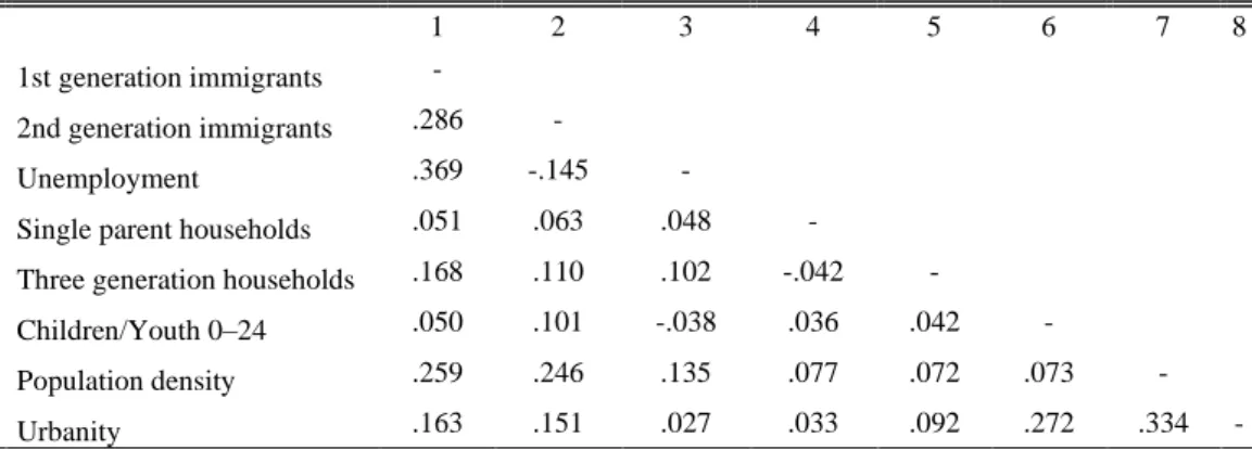
Table 2 below shows how most of the variables are correlated to each other showing the strongest correlations between first generation immigrants and unemployment.

Table 2 Variable Correlations

1 2 3 4 5 6 7 8

1 1st generation immigrants -

2 2nd generation immigrants .286 -

3 Unemployment .369 -.145 -

4 Single parent households .051 .063 .048 -

5 Three generation households .168 .110 .102 -.042 -

6 Children/Youth 0–24 .050 .101 -.038 .036 .042 -

7 Population density .259 .246 .135 .077 .072 .073 - 8 Urbanity .163 .151 .027 .033 .092 .272 .334 -

Note: all correlations show significance at p < .001

Spatial dependence

Spatial dependence, or autocorrelation as it sometimes is referred, is a spatial

process essential for the understanding of crime patterns (Chainey & Ratcliffe 2005) and other features of place. It is the degree to which the value of a variable

(14)

at one place is affected by neighbouring places and in general, this means that locations in close proximity are more likely to have similar values, compared to locations at larger distance (Chainey & Ratcliffe 2005). Crime levels at one location may for instance be influenced by, or at least related to, the adjacent area, and this is usually due to when it comes to crime anyway, that the underlying causes of crime can push crime rates in small areas (ibid.). This has been addressed in this thesis by creating buffer zones in two sizes around the centre of each square showing how many squares around one square that show high levels of each feature by using a cut-off point of two standard deviations. This leads to variables with buffer zones at 275 meters have a maximum value of 9, and buffer zones at 625 meters have a maximum value of 25. These numbers indicate how many squares in proximity show high values.

Considerations

Considering the variables applied in the present paper it is good to keep in mind that foreign-born individuals in the dataset from SCB also include adoptive children born abroad and children born abroad by domestic-born parents (SCB 2002). This mean that the current study’s terms, first and second-generation immigrants, do not fully embrace the whole picture even though adoptive children and children born abroad with domestic-born parents at present are very few. Another thing to keep in mind is the variable called three-generation households, that actually, as stated above, also include more features such as all other households where at least one person in the home does not have close relationships with anyone else in the household and are neither a child nor a parent, nor has a couple relationship with someone else in the household (SCB 2019).

Analytical strategy

First of all, the present study will use mean values and standard deviations in order to explain the structural characteristics of squares that coincide with vulnerable neighborhoods. These will be tested through independent t-tests in order to find out if they are significant or not. Based on these findings, different models will be tested using logistic regressions where the one with the highest explaining value, that is the highest pseudo R2,will be used as a statistical model. Built on this model using the b-coefficients, a vulnerable prediction value will be calculated by multiplying each coefficient with the standardised value of each variable and then adding them together. After each square have acquired a vulnerable prediction variable, these values are put back into the GIS-software in order to find clusters of squares with high values, indicating vulnerable neighborhoods.

RESULT

In the result below, vulnerable-, at risk- and particularly vulnerable squares are grouped together and labelled vulnerable squares with the values of yes (1) and no (0). In the result. the steps to answer the study question’s will thoroughly be explained and later discussed, from both a methodological approach and in the light of previous research and theoretical frames, in the following section, discussion.

Characteristics

To answer the first question, what are the characteristics of squares that coincide,

(15)

collection, mean values have been tested through independent t-tests. Table 3 below

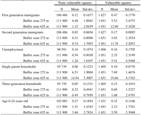
shows the mean percentage points of each variable and the mean value of both buffers at 275 meters (range 0-9) and 625 meters (range 0-25) for each variable. This analysis shows that squares in vulnerable neighborhoods have a fairly high share regarding foreign background and unemployment with similarity in the buffer zones. There are also slightly higher shares of three-generation housing and single parent households, where the latter also show higher proximity to other similar households.

Table 3 Independent T-test of mean values of squares that coincide with vulnerable neighborhoods or not according to the national collection.

None vulnerable squares Vulnerable squares N Mean Std.dev. N Mean Std.dev. First generation immigrants 106 486 0.12 0.1677 1 627 0.47 0.1770

Buffer zone 275 m 111 900 0.48 1.0042 1 651 5.53 2.4375 Buffer zone 625 m 111 900 1.15 2.0429 1 651 12.90 5.3420 Second generation immigrants 106 486 0.03 0.0656 1 627 0.17 0.0895 Buffer zone 275 m 111 900 0.31 0.8088 1 651 5.03 2.3554 Buffer zone 625 m 111 900 0.74 1.7093 1 651 11.78 5.2053 Unemployment 98 591 0.16 0.1974 1 606 0.34 0.1705 Buffer zone 275 m 111 900 0.54 0.9030 1 651 2.33 2.3199 Buffer zone 625 m 111 900 1.26 1.6107 1 651 5.41 4.5468 Single parent households 95 739 0.06 0.1223 1 605 0.10 0.0739 Buffer zone 275 m 111 900 6.51 1.9004 1 651 7.69 1.4676 Buffer zone 625 m 111 900 14.94 5.3007 1 651 19.66 4.1763 Three-generation households 95 739 0.05 0.1331 1 605 0.15 0.1019 Buffer zone 275 m 111 900 0.22 0.4941 1 651 0.69 1.2327 Buffer zone 625 m 111 900 0.49 0.7959 1 651 1.68 2.4793 Age 0-24 years old 102 083 0.27 0.1854 1 431 0.32 0.1166 Buffer zone 275 m 111 900 1.51 1.4345 1 651 2.23 1.7761 Buffer zone 625 m 111 900 3.46 2.7824 1 651 5.50 3.3048

Note: all values above show significance at p < .001

These results indicate that features in squares that coincide with vulnerable areas show higher concentrations of residents with both foreign background and unemployment, and this also in proximity to other squares. Households with single parents are not as strong indicator as three generation households, but nevertheless in proximity to similar households. There are a slightly higher share of children and youth in vulnerable squares.

A statistical model in progress

With the knowledge about the characteristics of squares that coincide with vulnerable neighborhoods, a statistical model will be created using logistic regression analyses in order to answer question two - How can we statistically,

trough socio-demographic data, identify vulnerable neighborhoods from the national collection? Numerous logistic regressions have been made in the effort of

finding the one model that from a theoretical point makes the most sense and at the same time shows a high pseudo R2-value. In the logistic regression analyses’ all variables have been standardised for better comparability.

(16)

Table 4 Logistic regression analysis showing B-values with vulnerable neighborhood (no/yes) as dependent.

Model 1 Model 2 Model 3

B sig. B sig. B sig.

Population density .381 .000 .347 .000 .234 .000 Urbanity .370 .000 .419 .000 .366 .000

Unemployment .712 .000 .054 .136

Single parent households’ .712 .000 .178 .000 Three generation households’ .368 .000 .158 .000 First generation immigrants’ .994 .000 Second generation immigrants’ .753 .000

Age 0 - 24 years old .051 .162

Nagelkerke R2 _.167 _.266 _.488

Note: standardised variables

The two foreign background variables accounted for most of the variance in vulnerable squares. As model 3 in table 4 is an example of, whenever foreign background come into the model, unemployment is no longer significant, and its B-value decreases.

Unemployment buffer 275m .685 .000 .636 .000 .015 .500 Age 0 - 24 years old buffer 275m .272 .000 .118 .000 -.016 .661 Single parent households’ buffer 275m .524 .000 -.274 .000 Three generation households’ buffer 275m .377 .000 .062 .007 1st generation immigrants’ buffer 275m .000 .653 .000 2nd generation immigrants’ buffer 275m .601 .000

Nagelkerke R2 _.171 _.216 _.584

Foreign background seems to account for much of the variability of vulnerable squares, also when looking at buffer zones of both 275- and 625 meters as seen in table 5 and table 6. The pseudo R2-values also increases for the buffer-models where it is highest for model three in table 6.

Unemployment buffer 625m .769 .000 .699 .000 .019 .378 Age 0 - 24 years old buffer 625m .405 .000 .099 .000 .124 .001 Single parent households’ buffer 625m .700 .000 -.109 .022 Three generation households’ buffer 625m .480 .000 .010 .668 1st generation immigrants’ buffer 625m .000 .685 .000 2nd generation immigrants’ buffer 625m .518 .000

Nagelkerke R2 _.248 _.318 _.602

(17)

After examining numerous logistic regressions, the final model was clear, indicating a pseudo R2- value at .62. Table 7 illustrate the final model where most of the variables are significant at a 5 percent level in model 3. This corresponds to research question two, the answer to which is that it is possible to statistically identify vulnerable neighborhoods from the national collection by using socio-demographic data.

Population density .382 .000 .273 .000 .028 .166 Urbanity .379 .000 .356 .000 .440 .000 Single parent households’ .171 .000 .093 .026 First generation immigrants’ .958 .000 .346 .000 Second generation immigrants’ .658 .000 .212 .000 1st generation immigrants’ buffer 275m .343 .000 2nd generation immigrants’ buffer 275m .474 .000 Unemployment buffer 625m .202 .000 Three generation households’ buffer 625m .031 .179 Age 0 - 24 years old buffer 625m .069 .034

Nagelkerke R2 _.163 _.460 _.621

Using a vulnerable prediction estimate

A vulnerable prediction value was calculated based on model 3 in table 7, by multiplying the b-coefficients with the standardised variables and creating a

vulnerable prediction variable. These values were then exported into the

GIS-software and added to a layer of squares. To answer question 3 and 4, if there are

areas which, statistically appear to be vulnerable based on the statistical model, but which are not classified so, and if there are areas that statistically do not appear as vulnerable based on the statistical model, but which are still classified so, a

cut-off point was set at 6.0369. This value was based on the mean value of the vulnerable prediction variable for squares that are classified as vulnerable according to the national collection, see descriptives in table 8.

Table 8 Descriptives of vulnerable prediction variable Vulnerable squares No Yes Valid 92 933 1 595 Missing 18 967 56 Mean -.0249 6.0369 Standard deviation 1.1723 2.4996 Range 11.85 13.41 Minimum -1.14 -.66 Maximum 10.71 12.75

After manually going through squares at both all bigger urban areas and smaller more rural areas of Sweden, four categories of changes were distinguished. This

(18)

step has then been done five times to make sure the measuring is the same every time. The first category (A), new free-standing areas consisting of at least four contiguous squares was easily notable. The second category (B), that was detected were also new areas, containing at least 4 contiguous squares, but that were adjacent to already classified areas from the national collection. The third category (C), shows already classified areas, reduced in size according to the statistical model. Finally, the fourth category (D), were areas that according to the national collection are vulnerable, but giving the statistical model, no longer are.

Table 9 Number of areas in each category.

Category N A 13 B 16 C 16 D 13 Category A

In the whole of Sweden, 13 new free-standing areas were found. Below, map 1, shows a part of the Swedish capital, Stockholm, where four new areas were found. The small area to the left, consisting of three squares does not count for a vulnerable area since a minimum of four squares were the chosen definition, but the one further down with eight squares do. The squares further down on the map is counted for two areas, one with four squares and one with 10 squares.

Category B

Sixteen new areas were found adjacent to already vulnerable areas. Map 2 shows a part of Gothenburg, the second largest city in Sweden, and here can be seen examples of two new areas matching category B. One in the middle top, and one further down in the middle, both consisting of ten squares each. Category B could also count as areas which can increase in size, but it may also be what geographically or linguistically, are new areas, as measured here, Kortedala and Angered Centrum, shown in map 2. Hence, in this category there may be some issues regarding the definition, where it can be hard to identify new areas in proximity to already vulnerable areas. Another example relating to issues are in Malmö (see map 3 on the next page), where five areas, according to the chosen definition, are discovered around and between three already vulnerable areas in Malmö, which challenge this subjective assessment.

(19)

Category C

In the third category, sixteen reduced vulnerable neighborhoods from the national collection were found. As map 4, showing another part of Gothenburg, illustrate there are areas that also can be reduced according to the model. Some areas can be reduced quite a bit as map 4 is an example of. Before, each of the 16 neighborhoods in category C consisted of an average of 40 squares and after using the prediction value the average size are 15 squares, which mean that they have been reduced with an average of 24 squares. Neighborhoods which are in proximity to the category B are not counted as a category C even if the original area is seen to decrease in size. There are nevertheless some issues in the measuring of category C, where it is a quite subjective assessment which can be hard to interpret as shown in map 5, an example of a vulnerable area in Halmstad, where it is hard to interpret if the amount of squares really are fewer or more since the predicted area goes further up north compared to the national collection. This type of area has in the result however not been classified as a category C.

Map 4 Example of category C in Gothenburg.

Map 6 Example of category D in Norrkoping. Map 5 Example of an area not matching the criteria

for category C in Halmstad.

Map 3 Example of areas matching the criteria for category B, but is hard to measure, in Malmö.

(20)

Category D

Thirteen neighborhoods from the national collection are, according to the model’s prediction value, no longer vulnerable. As can be seen in map 6 on the previous page, showing the city of Norrkoping, these two areas are quite easy to discover and there are no issues in determine their category.

DISCUSSION

Much of the previous research in the current study is allocated to crime and criminal behaviour and even though this study has a more direct link to structural characteristics than actual crime, the link to crime is still within the national collection as a subjective assessment. However, this study’s main aim is more methodological with the question of how we on a more objective way can measure vulnerable neighborhoods, rather than trying to find areas more criminogenic. The overall result of the current paper is in line with previous research and theoretical framework of social disorganisation theory where areas characterised with socioeconomic difficulties, population heterogeneity and family disruption are more crime prone than other residential areas (Anselin 2008; Sampson 2006; Samson et al. 1997), with the exception that the present study does not measure crime per se, rather police perceptions of areas with certain crime characteristics. Likewise, that there are differences in how the socio-structural measures are operationalised. Even so, the present study has identified that squares that coincide with vulnerable neighborhoods, according to the national collection, show higher rates of residents with foreign background, unemployed residents, single parent- and three generation households.

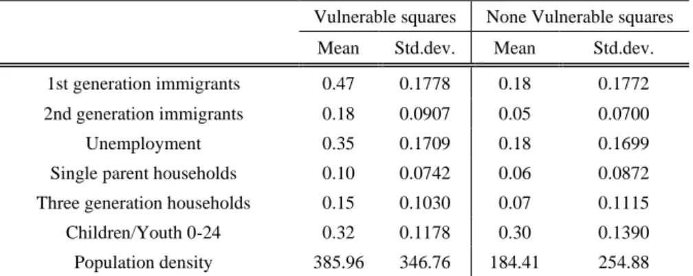
About fifty percent of the vulnerable squares appear in the three biggest cities in Sweden - Stockholm, Gothenburg and Malmö. Another forty-four percent of the vulnerable squares are to be found in larger urban areas in Sweden with a minimum of 40 000 residents. Previous research argues that city centres and areas with mixed land use and transport nodes often are more criminogenic than residential areas (Ceccato 2012; Sherman et al. 1989; Wikström et al. 2012). Though, vulnerable neighborhoods from the national collection in Sweden usually compose of residential areas and they show quite high crime levels and increased levels of feelings of unsafety compared to other residential areas (NCCP 2016) and appear therefore more alike inner-city areas. Though, given structural characteristics, the result of the current paper implies some differences between vulnerable neighborhoods classified by the police and other inner-city areas. With this in mind, it would be preferable to compare vulnerable squares with other urban squares, something that has been done using independent t-tests (see table A1); revealing higher shares of foreign background, unemployment, single parent- and three generation households in vulnerable squares compared to other urban squares. By testing multiple logistic regression models, the present study managed to find a model that explained more than about 60 percent of the variance in vulnerable neighborhoods classified by the national collection. One of the most interesting findings in the logistic regression analyses suggests that foreign background is the most important variable when predicting vulnerable neighborhoods from the

(21)

national collection. One can only speculate why this is, if it is some kind of criminal organisation or structure that might be more common among residents with foreign background, police bias or something completely different? Anyhow, the implication that foreign background appears more important than most variables, and unemployment particularly, is something that in similar ways also has been discovered in other studies (see for example Gerell 2017a). Bruinsma and colleagues (2013) also finds that ethnic heterogeneity, which most likely correlates with foreign background, has the most significant influence on different social disorganisation models on crime rates. Additionally, in the light of Merton’s strain theory, feelings of strain are dependent on where members of society come from and how they can achieve the common goals set by society (Merton 1938). Agnew (2001) develops this and imply that strain also occurs in combination of low social control and according to the theory of collective efficacy, neighborhoods with structural difficulties are less likely to practice informal social controls (Sampson et al. 1997); and therefore disorder and crime might be perceived higher in neighborhoods showing structural characteristics found in the present study. Another potentially important finding in the current study is regarding the various sizes of classified vulnerable neighborhoods from the national collection. They vary between 4 squares up to 76 squares1, and with larger areas found in bigger cities. The result of the predicted squares indicates that as many as 16 neighborhoods can be reduced in size, from an average of 40 squares down to an average of 15 squares. When only visually looking at the neighborhoods, sometimes smaller neighborhoods are very close in proximity to each other (see Eskilstuna for example in map A1), but still considered two neighborhoods and in other cases several neighborhoods are emerged, as in for example Malmö where the neighborhoods of Nydala, Hermodsdal and Lindängen are emerged as one in the national collection, originally consisting of 32 squares. These discrepancies have the potential to be reduced when measuring in a more objective way, especially if more measures are added.

The modifiable areal unit problem

Previous research has highlighted the importance regarding the size of the unit to be studied and Oberwittler and Wikström (2009) argue that the unit of analysis seldom is a problem when studying individuals, but when studying the environment, the unit of analysis becomes far more complex. The problems connected with the choice of area units are well known in geography and other spatially oriented social sciences as the “modifiable areal unit problem” (MAUP) and one basic issue identified in MAUP is the zonation effect; which relates to the difficulty of drawing significant boundaries within an area, which reflect the spatial patterns of important variables (Oberwittler & Wikström 2009). This is something that often are a problem when using administrative boundaries such as census tracts or other official data (ibid.). Researchers argue that the use of smaller geographical units is to prefer because they are less prone to be deficient due to that they tend to show higher internal homogeneity (see for example Gerell 2017b; Oberwittler & Wikström 2009). Even though the current study uses pre-defined administrative boundaries from SCB, this issue is still addressed by using small units of analysis, smaller than the often-used census tracts. Yet, there is one finding in the current study that question this issue. The logistic regressions revealed, that when foreign background is accounted for, unemployment and three generation households are

(22)

better measured using bigger units, here used by a buffer of 625 meters from the square middle. This might indicate that when variables are used separately, the smaller size is sufficient, but collectively, some variables are better measured using larger units.

Another issue found in MAUP is the scale effect or aggregation bias, regarding the establishing of appropriate size of units where correlations relevant to the variables depends on the level of spatial aggregation employed in the analysis (Gerell 2017b; Oberwittler & Wikström 2009). The bigger the area, the more problem comes with for example non-residential land use in one part of the area which in another part of the area may be irrelevant for a household variable (Oberwittler & Wikström 2008). Therefore, many researchers argue for “smaller is better“ (see for example Gerell 2017b; Oberwittler & Wikström 2009). The small units of the current study arguably have the potential to measure the structural characteristics accurately within each square.

Some of the present study’s variables are similar to other variables used in other studies, combined as a concentrated disadvantage index. Gerell and Kronkvist (2017) uses an index of concentrated disadvantage with correlated variables, among them unemployment, single parent households, foreign-born residents and median income, to units of the size of subdistricts in the city of Malmö. In the current study, creating an index like concentrated disadvantage has not been an option due to that the highest Cronbach alpha value generated of variables connected to concentrated disadvantage landed on .534; this when including variables of first- and second-generation immigrants, unemployment and three second-generation households, even lower alpha value when adding single-parent households. This value indicates a too low internal consistency to represent a combined index. This finding, suggests some kind of aggregation bias, but this might be due to that many similar studies analyses one or two cities and the present study look at an entire country; where it is more likely that there will be greater variations in how variables are related.

One key aspect regarding the profits made from studying smaller units, is that they are less likely to stigmatise entire communities or residential areas (Weisburd et al. 2014). If most of the criminal activity only are related to very small areas or places in a residential area, it is quite misleading to label entire residential areas as criminogenic. Smaller areas often account for the highest level of crime, which varies between contexts and therefore, it is important to have a locally based understanding of the link between crime and urban characteristics (Wuschke & Kinney 2018). Hence, aggregating crime data to the squares in the present study have the prospective to more accurately map vulnerable neighborhoods which further could make it less stigmatising.

Study limitations

Even with a well-documented methodology and a clear approach, the current paper does not stand out more than others concerning the occurrence of limitations. The most limited part of the current study is when manually going through squares using the prediction value in the GIS-software. This is yet another subjective assessment and therefore might be seen as an inconsistency from the aim of this paper which were supposed to be a more objective assessment than the national collection. However, a totally objective assessment will probably be hard to conduct, and it is perhaps not possible to completely move away from a subjective assessment.

(23)

CONCLUSION

The present study contributes to the academic knowledge regarding statistics of micro-places and vulnerable neighborhoods. The aim of the study was to use a statistical approach to objectively measure vulnerable neighborhoods in Sweden compared to how it today is being done. As expected with regards to social disorganisation theory, the current study shows that some specific features are more common in vulnerable neighborhoods and the analyses revealed that some areas in the national collection can either decrease in size or not be classified as vulnerable at all. At the same time, the analyses also imply new areas with similar characteristics that are not counted for in the national collection. By the means of only using structural data of urban neighborhoods, the result of this study indicate that it is possible to capture features of the classified vulnerable neighborhoods from the national collection, though the present study’s model does not explain all the variance. In the future, by aggregating crime data, this statistical model has the potential to identify vulnerable neighborhoods more effectively and accurately than what today is being done. In the future case of aggregating crime data, it would also be interesting to study the three separate classifications of the national collection more in depth. Future research should also consider if and how it is possible to aggregate some kind of fear-of-crime data in order to get a deeper understanding. A key implication of why it may be essential with a more objective assessment of vulnerable neighborhoods is that there probably are significant differences between police perceptions from working in big cities compared to more rural areas, but also amongst the bigger cities. That is, an officer in a smaller city might feel a serious event is huge which may affect his perception of a certain area more and for a longer period of time, compared to an officer in a big city that deal with that kind of events more often. Nevertheless, even with a more objective assessment, one ought never to dismiss police perceptions regarding their work in vulnerable neighborhoods. Lastly, an additional important aspect for attempting to find a more objective way to map and classify vulnerable neighborhoods is to reduce the risk of labelling neighborhoods as criminogenic and along with that also its residents living there. Both Farrington (1977) and McAra & McVie (2012) explain that juveniles living in neighborhoods with socioeconomic difficulties are at higher risk of police encounters which might be due to what Sampson (1986) argues, there being higher police presence in these types of neighborhoods. In the light of the labelling perspective, it is important to consider the result related to this study’s first question regarding the structural characteristics found in vulnerable squares classified by the national collection. With regard to the present study’s result, suggesting there are significantly higher shares of residents with foreign background in vulnerable squares, it is important to keep in mind what Sampson and Raudenbush (2004) found in their study - that social structures and cultural stereotyping is a more powerful predictor of perceived disorder, rather than the actual disorder. Therefore, the move towards a more objective assessment may be of importance.

(24)

REFERENCES

Agnew, R. (2001). Building on the foundation of general strain theory: Specifying the types of strain most likely to lead to crime and delinquency. Journal of

Research in Crime and Delinquency, 38: 319-361.

Anselin, L., Griffiths, E., & Tita, G. (2008). Crime mapping and hot spots analysis. In: Wortley, R., & Mazerolle, L. (eds). Environmental Criminology and Crime

Analysis. New York: Willan Publishing. Pages 97–116.

Bruinsma, G., Pauwels, L., Weerman, F., & Bernasco, W. (2013). Social Disorganization, Social Capital, Collective Efficacy and the Spatial Distribution of Crime and Offenders: An Empirical Test of Six Neighbourhood Models for a Dutch City. The British Journal of Criminology, 53(5), 942.

Brunton-Smith, I., & Sturgis, P. (2011). Do Neighborhoods Generate Fear of Crime? An Empirical Test Using the British Crime Survey. Criminology, 49(2), 331–369.

Ceccato, V. (2012). The Urban Fabric of Crime and Fear. In: Ceccato, V. (eds.).

The Urban Fabric of Crime and Fear. Dordrecht: Springer Netherlands, 2012.

Pages 3–33.

Chainey, S., & Ratcliffe, J. (2005). GIS and Crime Mapping. Chichester, West Sussex: John Wiley & Sons LTd.

Crocker, R., Webb, S., Skidmore, M., Garner, S., Gill, M., & Graham, J. (2018). Tackling local organised crime groups: lessons from research in two UK cities.

Trends in Organized Crime, 1-17.

Davies, T., & Bowers, K. (2018). Street Networks and Crime. I: Bruinsma, G.& Johnson, S. D. (red.). The Oxford Handbook of Environmental Criminology. Oxford University Press. S. 545-576

Farrington, D. (1977). The effects of public labeling. British Journal of

Criminology, 17:112-125.

Gerell, M. (2017a). Collective efficacy and arson: the case of Malmö. Journal of

Scandinavian Studies in Criminology and Crime Prevention, 18(1), 35–51.

Gerell, M. (2017b). Smallest is Better? The Spatial Distribution of Arson and the Modifiable Areal Unit Problem. Journal of Quantitative Criminology, 33(2), 293– 318.

Gerell, M., & Kronkvist, K. (2017). Violent Crime, Collective Efficacy and City-Centre Effects in Malmo. British Journal of Criminology, 57(5), 1185–1207. Kim, Y. A. (2018). Examining the Relationship Between the Structural Characteristics of Place and Crime by Imputing Census Block Data in Street Segments: Is the Pain Worth the Gain? Journal of Quantitative Criminology, 34(1), 67–110.

(25)

Lilly J. R, Cullen F. T, & Ball R. A, (2011). Criminological Theory: Context and

Consequences. 5th ed. Thousand Oaks: Sage Publications.

Maxfield, M. G. & Babbie, E. R. (2015). Basics of research methods: for criminal

justice and criminology. Boston: Cengage Learning, Inc, 2015.

McAra L. & McVie S. (2012). Negotiated order: The groundwork for a theory of offending pathways. Criminology and Criminal Justice 12(4): 347-375.

Merton, R. K. (1938). Social structure and anomie. American Sociological Review,

3: 672-682.

NCCP (2009) Otrygghet och segregation. Bostadsområdets betydelse för

allmänhetens otrygghet och oro för brott. Rapport 2008:16. Stockholm:

Brottsförebyggande rådet.

NCCP (2015a. Börja med en kartläggning! Kunskapsbaserat arbete i utsatta

områden. Stockholm: Brottsförebyggande rådet.

NCCP (2016). Insatser mot brott och otrygghet i socialt utsatta områden. En

kunskapsöversikt. Rapport 2016:20. Stockholm: Brottsförebyggande rådet.

NCCP (2018). Utvecklingen i socialt utsatta områden i urban miljö 2006–2017. En

rapport om utsatthet, otrygghet och förtroende utifrån Nationella trygghetsundersökningen. Rapport 2018:9. Stockholm: Brottsförebyggande rådet.

NCCP (2019). Dödligt våld i Sverige 1990–2017. Omfattning, utveckling och

karaktär. Rapport 2019:6. Stockholm: Brottsförebyggande rådet.

Oberwittler, D. & Wikström, P-O. (2009). Why Small is Better: Advancing the

Study of the Role of Behavioral Contexts in Crime Causation. In: Weisburd, D.,

Bernasco W., & Bruinsma G. J. N. (eds). Putting Crime in Its Place: Units of

Analysis in Geographic Criminology, 35-59. New York: Springer.

Police (2017). Utsatta områden – Social ordning, kriminell struktur och

utmaningar för polisen. Stockholm: Nationella operativa avdelningen,

Underrättelseenheten.

Police (2019). Kriminell påverkan i lokalsamhället - En lägesbild för utvecklingen

i utsatta områden. Stockholm: Nationella operativa avdelningen, Underrättelseenheten.

Rengert, G. F., & Lockwood, B. (2009). Geographical Units of Analysis and the

Analysis of Crime. In: Weisburd, D., Bernasco, W., & Bruinsma, G. (eds). Putting Crime in its Place - Units of Analysis in Geographic Criminology. New York:

Springer. Pages 109 – 122.

Sampson, R. (1986) Effects of socioeconomic context on official reaction to juvenile delinquency. American Sociological Review, 51: 876-885.

Sampson, R. J. (2006). How does community context matter? Social mechanisms