Fast calculation of some important dimensioning factors of the railway power supply system

FAST CALCULATION OF SOME IMPORTANT DIMENSIONING

FACTORS OF THE RAILWAY POWER SUPPLY SYSTEM

Lars Abrahamsson

Royal Institute of Technology

Stockholm, Sweden lars.abrahamsson@ee.kth.se

Lennart Söder

Royal Institute of Technology

Stockholm, Sweden lennart.soder@ee.kth.se

Abstract – Because of environmental and economical

reasons, in Sweden and the rest of Europe, both personal and goods transports on railway are increasing. Therefore great railway infrastructure investments are expected to come. An important part of this infrastructure is the railway power supply system. Exactly how much, when and where the traffic will increase is not known for sure. This means investment planning for an uncertain future. The more uncertain parameters, such as traffic density and weight of trains, and the further future considered, the greater the inevitable amount of cases that have to be considered. When doing simulations concerning a tremendous amount of cases, each part of the simulation model has to be computationally fast – in real life this means approximations. The two most important issues to estimate given a certain power system configuration, when planning for an electric traction system, are the energy consumption of the grid and the train delays that a too weak system would cause. In this paper, some modeling suggestions of the energy consumption and the maximal train velocities are presented. Two linear models, and one nonlinear model are presented and compared. The comparisons regard both computer speed and representability. The independent variables of these models are a selection of parameters describing the power system, i.e.: power system technology used on each section, and traffic intensity.

1. Introduction

During the last decades, the railway has in many countries experienced a renaissance. The main reasons for the expansion of the railway are environmental and economical. This, in turn, has increased the interest in railway grid research.

When making a decision about the future railway power supply system, possible under-investments or over-investments need to be estimated in an appropriate manner. The costs of over-investments are simply put: the price difference between the investment cost of the "too strong" and the "sufficiently strong" power system configurations. Costs that are related to under-dimensioning are somewhat more subtle, though. Some examples will be mentioned in the following.

While a voltage drop in the ordinary power system would cause occasional disconnections of customers, it would in the power supply system of the railway simply cause the

trains to run slower. The slowing down of trains do, however, immediately lead to costs – either by lower incomes due to reduced competitiveness on the transportation market – or for greater voltage drops, disturbed, or even modified time tables. With the trend of increasing energy prices in mind, power losses might be as important to study as delays caused by low voltage when looking into the future. Therefore, the initial focus on under-investment costs will be set to train velocities limited by the power system, as well as differences in energy use – losses will vary, as also train power demand – between different power system solutions.

The objective of this paper is to present an idea of how to pick out relevant information of the outputs of a basic simulation method (TTS), and by presenting the input variables to an Approximator (TTSA) estimate these relevant outputs, see Figure 1 (Main results). Relevant outputs are here chosen to be the maximal train throughput velocity, as well as the corresponding energy consumption of the system, for a given train traffic and electric power supply system. The main ideas behind TTS, its model, as well as TTSA, and its accuracy and ability to generalize the results, are presented.

Fig. 1 – Overview of the main purpose of the paper A further developed TTSA (box C in Figure 1) approximating main results (box E) from TTS (box B), is planned to be used in a future investment planning tool. Planning will be done for several years ahead, allowing investments to be done stepwise. This planning tool should in the end be able to manage a huge amount of uncertain variables, such as: train types, train weights, locomotive types, energy prices, increasing or decreasing demand, taxes, the economical situation, and so forth. All the possible combinations of realizations of variables like these cannot be simulated (box B), because it would demand too much time. The aim is to use results from a limited number of TTS simulations to determine parameters for the TTSA model in box C. With this approach, the much faster TTSA model can be used for a large amount of scenarios.

2. Train Traffic Simulator (TTS)

The aim of TTS is to, as accurate as possible, simulate a certain traffic and a certain infrastructure.

Modeling

Electrical and Mechanical Power, for Each Time Step In this part of the paper, the system of equations to be solved for each time step is presented. A great part of the modeling is the same as in [1,2], and therefore only additional and updated equations will be presented here. The maximal tractive force of an Rc locomotive is a function of the catenary voltage,

U

, and the velocity of the train that it is hauling,

v

. The function can be expressed as a polynomial 2 ,max 1 2 3 4 5 2 3 3 4 6 7 8 9 4 5 5 10 11 12 13 2 2 3 2 4 14 15 16

,

motor

F

c

c U

c v

c Uv c v

c v U

c v

c v U

c v

c v U

c v

c v U

c U

c U v c U v

c U v

= +

+

+

+

+

+

+

+

+

+

+

+

+

+

+

+

+

2

₊

0

=

(1)

where the parameters can be obtained from data sheets [6] using least squares fitting. The motor force can be modeled as

(

)

,max

4

1

if

0

0

if

motor J motor

F

K

a

Br

F

Br

ζ

⎧

−

+

= ⎨

≠

⎩

(2)

where

ζ

is the slippage ratio [8],

K

_J is related to rotational inertia [8], is the acceleration, and is a variable that will be described in the method part. The adhesive tractive force between train and rail,

a

Br

, ,

7.5

0.161

44 3.6

tract adh adh drive

F

m

g

v

⎛

⎞

=

⎜

_⎝

+

₊

⎟

_⎠

(3)

for dry rail and

, ,

3.78

23.6

tract adh adh drive

F

m

g

v

⎛

⎞

=

⎜

_⎝

₊

⎟

_⎠

(4)

for wet rail, where is the gravitational constant, and is the mass on the driving axles of the train [8]. The effective tractive force

g

, adh drive

m

{

,

}

min

,

tract motor tract adh

F

=

F

F

(5)

because it is indifferent how strong the engine is if there is no grip [8]. The train resistive force due to mechanical and air resistances,

2 ,

air mech

F

= +

A

Bv Cv

+

(6)

where

A

,

B

, and

C

are train dependent [8]. The

resistive force due to grades

grades

F

= ⋅ ⋅

m g incl

(7) where

in

is the inclination of the track. The total resistive force is simply

cl

,

res air mech grades

F

=

F

+

F

. (8)

And

(

)

(

)

, ,

1

tract res adh drive adh drive

brake

F

F

m

m m

a

a

−

⎧

⎪

₊

₋

₊

= ⎨

⎪

⎩

H

₍₉₎

the first case if , the second if , and where is the total train mass [8], is the relative factor accounting for rotational inertia of the unbraked wheel sets [8], and will be described in the braking part.

0

Br

=

Br

≠

0

m

H

brake

a

The mechanical power of the motor

(

1

)

motor motor

P

=

F

v

+

ζ

(10)

[8]. The electrical power demand

D motor

P

=

P

(11)

which implicates an assumption of a lossless motor. The DC voltage of the motor,

max 14

min 1,

min 1,

di base kV

v

U

U

E

v

U

α

⎧

⎫

⎧

=

⋅

⎨

⎬

⋅

⎨

⎫

⎩

⎭

⎩

⎬

⎭

(12)

which is a wiser modeling when allowing greater voltage drops [11].

In converter stations with several converters of the same kind, , , and (the total active, reactive, and 50 Hz side reactive power generations, respectively) can simply be divided by the number of converters,

#

, in order to give the proper

U

and

G

P

Q

_G

Q

₅₀ conv

ψ

values [10].

( )

( )

2 50 2

#

1

arctan

3

#

#

arctan

#

m G q conv m m q conv g G q conv g g G q conv

P

X

Q

U

X

P

X

Q

U

X

ψ

= −

−

+

−

+

(13)

Both

U

m and

U

g are assumed to be at nominal voltage levels constantly. The phase shift on the 50 Hz side of the converter due to train power consumption is, according to [10],

( )

0 50 50 2 50 50

1

arctan

.

3

G m

X P

U

X Q

θ

=

θ

−

−

(14) The Braking

The problem would have grown tremendously if the driving behavior would have been subject for optimization with respect to time. In order to avoid the time dimension of the problem, the driver is assumed to be aggressive. When accelerating, he/she does it as hard as ever possible. Braking, on the other hand, demands a more sophisticated modeling in order to be able to stop at the train stations. In order to determine the shortest braking distance for a given initial velocity, a small optimization problem was set up. The braking acceleration was constrained to

m/s2, while was constrained to be nonnegative. The figure

0.

m/s2 is due to comfortability reasons and according to [4], there is never any problem achieving that retardation level. The position,

0

≥ ≥ − .85

a

0

v

85

p

, was constrained to lie within

0

≤ ≤

p

p

_station. The remaining constraints were as follows

{

}

2 1 1 1

2

,

1

,

2, 3,...,

t t t t t t t t t station t start t t t t t t station t t

p

p

v

a

p

p

p

p

v M

v

a

t

v

v

a

t

t

z

p

p

− − − ∀

Δ

=

+ Δ +

≥

−

≥ −

+ Δ

=

⎧

= ⎨

_{+ Δ}

_∈

⎩

=

∑

−

max (15)

where index

t

∈

{

1, 2,...,

t

_max

}

is time step index,

M

is a large number (in this case

1000

), and is the time step length. The value of must like

t

Δ

max

t

p

_station be big enough for the train to have time and place to stop. The second constraint remedies the phenomenon in discretized time that the position might be reduced when traveling forward if the retardation turns bigger than suitable for the problem. The third constraint ensures that the train stops at the station. The objective

z

is minimized.

This LP problem is solved for all integer velocities

v

_start between and

160

km/h, because it is the lowest that gives feasible solutions,

160

because Rc locomotives rarely go faster. The braking accelerations are stored as a discrete function

61

61

[

,

]

brake start

a

v

t

to be used in TTS later on, paired with the critical braking distance, . However, these critical distances does not really form a smooth

function of

brake

d

start

v

because of the time discretization. Therefore, the trend is extracted by least squares fitting into a sixth grade polynomial of

v

_start.

The Method

The Newton Raphson method of [1,2] did soon turn out to be too weak for these nonlinear models. In TTS, whose working idea is illustrated in Figure 2, Matlab mainly does the bookkeeping. GAMS is a powerful optimization program that is used for solving the system of nonlinear equations for each time step. The objective function of the GAMS program is the sum of the squared two-norms of the power flow error vector and the reactive power flow error vector, but could be chosen differently.

In order to reduce the computation complexity of the system of nonlinear equations, GAMS is programmed to use , the prior time step velocity, rather than the in the presented models assumed . Since is a parameter, and would, if introduced, be a variable depending on that in turn depends intricately on several other variables, the simplification is obvious. Moreover, will normally not change that much between two small consecutive time steps. Doing the same with, e.g.,

U

would be harder to justify – especially for weak BT power systems. The consecutive time steps are thus connected by

1 t

v

₋ t

v

v

_t−1

v

_t t

a

v

(

1 1

)

1 2 1

,

2

t t t t t t t t t t t t t

a

SOE p

v

v

v

a

p

p

v

a

− − − −

=

=

+ Δ

Δ

=

+ Δ +

(16)

where denotes the system of equations in the Modeling part.

SOE

Fig. 2 – Main ideas of the work flow of TTS The TTS time table (unidirectional traffic intensity) remains as in [1,2], i.e., a train is let loose in the start every nth minute, and once the entire track is filled up with trains the forthcoming train to let loose gets a label. When the labeled train reaches its final destination, the TTS simulation halts. The precalculated braking schedules that are described in the model section are used as follows. Before solving the equations, TTS checks if there is time to brake for any train. It is considered time to brake when

( )

0

<

p

_station

− <

p

_t

d

_brake

v

_t

+ Δ

v

_{t t}, where is a sort of insecurity factor due to the discrete time model. If there is time for a train to brake, then the parameter is raised one step and is stored as . This is done for

t t

v

Δ

0

Br

=

t

v

v

_brake

bookkeeping of train braking time and choosing an appropriate braking schedule. Matlab thereafter checks trains with parameter . The parameter is raised one step for the forthcoming time step. The braking acceleration is then determined by

0

Br

>

1

,

2

1

,

2

t brake brake t brake brake t

a

a

v

Br

a

v

Br

=

⎡

_⎣

⎡

_⎢

⎤

_⎥

⎤ +

_⎦

+

⎡

_⎣

⎢

_⎣

⎥

_⎦

⎤

_⎦

(17)

because the braking schedules are only computed for integer velocities. Five minutes after that has reached zero, is again set back to zero and the train can start accelerating, aiming for the next station on the track.

t

a

Br

3. The Approximator (TTSA)

The aim of the TTSA is to construct a method of retrieving reliable results fast, much faster than would be possible in TTS.

The Dependency Models

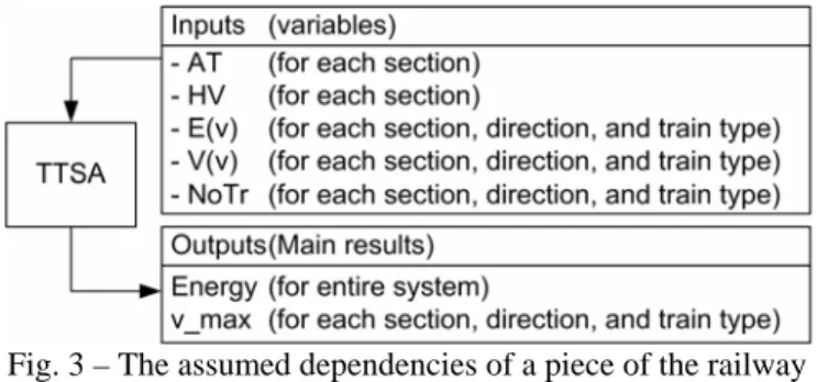
The inputs (Box A in Figure 1) chosen to be variables in this paper were: the catenary type (BT or AT [1,2]), the option of having an HV transmission line (130 kV 2-phase line [1,2]), and the traffic intensities quantified into three measures. The choice of catenary type,

AT

, as well as the HV line option,

HV

, are binary variables that tells whether the power supply system has AT catenaries or not, and HV transmission line or not, respectively. There is one such

AT

and

HV

pair for each section in the railway power system. The traffic intensity is described by

, the average velocity, and , the variance of the mean velocities, both of them taken over all trains (subscript

T

) during a certain time window (subscript ). The third traffic intensity measure is , the number of trains. There is one such

(

)

(

,

T t t

E

E v T

)

)

(

)

(

,

T t t

V

E v T

t

NoTr

( )

E v

, , and triplet for: each train type, each track section, and both traveling directions. Apart from the electromechanical properties, also the classification of trains as either "accelerating" or "speed-maintaining" is a train type demarcation. A train is classified as "accelerating" on a specific section if it is stopped on the section border before entering the section. This is indeed a crude measure, and a future TTSA should be able to handle trains stopping several times in each section. Track section borders are defined by the converter station locations in the non-HV cases, e.g., in Figure 4 there are two sections.

( )

V v

NoTr

Fig. 3 – The assumed dependencies of a piece of the railway grid

In the simple example of this paper, mixed traffic is not studied, and all trains have the same such that the variances can be neglected. Moreover, all trains are "accelerating" so no separation between "accelerating" and "speed-maintaining" trains is needed. The general dependency model assumed for TTSA in this paper is illustrated in Figure 3.

(

,

t t

E v T

)

There are two kinds of outputs of TTSA, see Figure 3. First, the average energy consumption of the power system. Second, , the maximal attainable velocity for each section, direction, and train type. In this paper, all outputs are assumed to depend on all inputs. Since the power flows are not local in the power system, especially not when using AT and/or HV, the energy consumption is hard to separate into section components. It is however tempting to, in a future improved TTSA, model at least the s as functions merely of the traffic in the concerned section.

max

v

max

v

Three different methods of modeling how the assumed outputs depend upon the assumed inputs are proposed. The input and output assumptions are illustrated in Figure 3. The first model,

M

1

, assumes a linear dependency

,

approx

i i k k

out

= +

b

∑

in w

_{i k}, where

i

is output index, is input index, and and are parameters to be determined by minimizing the mean square of the error, , in an optimization program. The second model,

k

, i k

w

b

_i approx i

out

−

out

_i

2

M

, is also linear; with the same inputs, outputs, and parameters. In

M

2

, however, the parameters are determined by the Matlab Neural Network (NN) Toolbox algorithm "trainb" (batch learning). In other words,

2

M

is a single layered neural network with inputs , outputs , and have

k

in

approx i

out

i

neurons with linear transfer functions. The third model,

M

3

, is a nonlinear NN with two layers. The first, "hidden", layer has transfer functions, and the second (output) layer has linear transfer functions. According to the theory [5,9], this kind of network can be used as a general function approximator, given sufficient neurons in the hidden layer. The hidden layer was chosen to have

3

neurons, the linear (output) layer naturally has

tanh

i

neurons, and the network is trained using the "trainbr" (Bayesian regularization backpropagation) algorithm with an error goal of

10

−5.

Both the and data are normalized to lie in the interval

k

in

out

_i

[ ]

−

1,1

before training and testing the approximators. Furthermore, the

128

TTS results are separated into one randomly chosen training set of size

32

, and one remaining test set. The figure

128

comes from four different power system configurations and

32

different train departure periodicities

n

leaping from to , from

by

1.

to

30

, and from

33

by

3

to

60

(minutes).

6

20

21

5

The main difference by minimizing the mean square error (MSE) by an optimization algorithm compared to a NNs algorithm is that one can perform a fewer amount of iterations in a wiser way in the latter case. Of course, that leads to a non optimal MSE, but hopefully a model that better generalizes the behavior of the system studied.

4. Numerical Example on a Test System

System Configuration

The system that the TTS has simulated is a three city test system (Figure 4), mainly using the same ideas as in [1,2]. In the test system the converters are of type Q48/Q49 [7]. In the HV case, there are converter stations situated in City1 and City2 with converters in each. In the non-HV case, there are three converter stations – one in each city – with converters in each. In the test system, trains denoted "F1 Mixed" in [8] are used. was set to minutes in TTS. The stretch "City Distance" was

50

km.

6

4

t

Δ

0.1

Fig. 4 – An illustration of the test system

The inclinations on the test system are inspired by the stretch between Luleå and Bastuträsk. The hight curve is measured from a graph [3] every km whereafter the inclinations are calculated. The rail is assumed to be dry. The slippage ratio,

6.25

th

ζ

, is for simplicity set to be zero, and

4

K

_J is assumed to be

10750

N, a typical figure [8]. Moreover, the 50 Hz sides of the converters stations have no load angle like in [1,2]. Finally, is assumed to equal zero.

50

0

θ

=

o

_H

Results and Conclusions

In Figure 5 there are two plots of selected TTS data: one for the strongest system with the lightest load, and one for the weakest system with heaviest load simulated. The variables

,

v

P

_D,

Q

_D, and

U

are shown for the labeled train while driving the first

100

km. is a part of box E in Figure 1, the others of box D.

v

is normalized by

150

km/h,

v

D

P

and

D

Q

are normalized by

5

MW/MVAr, and

U

by

16

kV. The inclination of the track (a part of box A) is included to show its influence,

in

is scaled so that corresponds to per mill.

.5

cl

−

1,1

10,10

−

0 20 40 60 80 100 0 0.2 0.4 0.6 0.8 1 km normalized data AT=0,HV=0,n=6 v P_D QD U incl incl=0 0 20 40 60 80 100 0 0.2 0.4 0.6 0.8 1 km normalized data AT=1,HV=1,n=60 v P_D QD U incl incl=0

Fig. 5 – A selection of TTS data

The remainder of this section is devoted to TTSA. As one would have expected, the linear NN tends to coincide with the GAMS solution when training it for thousands of iterations and when the MSE goal is set small. The errors of the mean energy of such an Approximator were about for the training set and for the test set. The errors of the maximal velocities were negligible compared to the approximation errors of the energy. For a less trained linear NN, the errors on the output vector are more equally spread and the generalization is slightly better. The approximation errors for the nonlinear NN are evenly spread, with norms similar to the linear cases.

5

10

−

4

10

−

In a minor modification of the GAMS program, certain

w

and were set to zero in order to determine whether the maximal velocity of a section could be modeled as depending only on the traffic on that very section. This assumption would be reasonable because of the voltage control on the section borders. Simulations shown just a slight decrease in approximator performance, so one could conclude that the traffic of neighboring sections do not affect each other much.

b

The computation times for making one estimation might be of interest. Since it is unfair comparing different programs, the both NNs are compared. By the usage of "tic" and "toc" in Matlab, the approximation calculation times turned out to be less than in the linear network and less than seconds in the nonlinear, on average, on an IBM X40 portable computer.

2

3 10

⋅

−

2

1.6 10

⋅

−

References

[1] L. Abrahamsson, "Basic Modeling for Electric Traction Systems under Uncertainty", UPEC (Universities Power Engineering Conference) 2006, 2006.

[2] L. Abrahamsson, "Operation Simulation of Traction Systems", to be published in the Comprail 2008 preeceedings, presented orally at Comprail 2006, 2006.

[3] Banverket, Track profile Luleå-Borlänge (original title in Swedish), 2007.

[4] E. Friman, Personal communication, 10 January 2007, M.Sc. E.E. at the Swedish Railway Administration (Banverket), Borlänge.

[5] K. Gurney, "An Introduction to Neural Networks", CRC Press, 2003, p. 78.

[6] N. Jansson, "Electrical Data for the Locomotive Types Rc4 and Rc6" (original title in Swedish), TrainTech, Solna, 2004.

[7] H. Kols, "Frequency Converters for Railway Feeding" (original title in Swedish), BVH 543.17000, Banverket, 2004.

[8] P. Lukaszewicz, "Energy Consumption and Running Time for Trains" Ph.D. Thesis, Division of Railway Technology, KTH, Stockholm, 2001.

[9] Matlab online help, Neural Network Toolbox, www.mathworks.com/access/helpdesk/help/toolbox/nn et/backpro4.html, 9 March 2007.

[10] M. Olofsson, "Optimal Operation of the Swedish Railway Electrical System", Ph.D. Thesis, Electric Power Systems, KTH, 1996.

[11] S. Östlund, Personal Communication, 2 February 2007, Professor at the division of Electrical Machines and Power Electronics, KTH, Stockholm.